Predicting rock mass rating ahead of the tunnel face with Bayesian estimation

The rock mass rating (RMR) system plays a crucial role in geomechanics assessments for tunnel projects. However, conventional methods combining empirical and geostatistical approaches often yield inaccuracies, particularly in areas with weak strata such as faults and karst caves. To address these uncertainties and errors inherent in empirical techniques, we propose a progressive RMR prediction strategy based on the Bayesian framework. This strategy incorporates three key components: 1) Variogram modeling: utilizing observational data from the excavation face, we construct and update a variogram model to capture the spatial variability of RMR. 2) TSP-RMR statistic model: we integrate a TSP-RMR statistical model into the Bayesian sequential update process. 3) Bayesian maximum entropy (BME) integration: the BME method combines geological information obtained from tunnel surface excavation with tunnel seismic prediction (TSP) data, ultimately enhancing the RMR prediction accuracy. Our methodology is applied to the Laoying rock tunneling project in Yunnan Province, China. Our findings demonstrate that the fusion of soft data and geological interpretation significantly improves the accuracy of RMR predictions. At selected prediction points, the relative error of our method is less than 15% when compared to the traditional Kriging method. This approach holds substantial potential for advancing RMR estimation ahead of tunnel excavation, particularly when advanced geological forecast data are available.

1 Introduction

The surrounding rock plays a vital role in tunnel engineering as it concerns both safety and efficiency in the design and construction phases. During construction, the variety of geological conditions might lead to serious hazards or collapses, resulting in casualties and financial losses. Hence, an accurate rock quality assessment ahead of the tunnel surface to dynamically revise the support schemes could decrease the hazards during construction.

To accurately reflect the quality of the surrounding rock, conventional rock mass classification systems are still employed in current tunnel construction practice, and a variety of rock mass classification systems have come forward to evaluate the quality of the geological conditions. Standard rock classification methods include the Q-system classification, rock mass rating (RMR) classification (Bieniawski, 1973), geological strength index (GSI) classification (Hoek et al., 1997), and the basic quality (BQ) approach. Among them, RMR is one of the most extensively used rock mass classification systems because of its comprehensiveness of the indicators and convenient application. The RMR system consists of six main indicators: the uniaxial compressive strength (UCS) of rock material, rock quality designation (RQD), joint and bedding spacing, joint condition, groundwater conditions, and orientation of discontinuities for the opening axis.

The current practice in predicting RMR involves a comprehensive evaluation of the rock mass based on several parameters, which typically include the uniaxial compressive strength of the rock material, RQD, spacing of discontinuities, condition of discontinuities (such as persistence, aperture, roughness, infilling, and weathering), groundwater conditions, and the orientation of discontinuities. For instance, Niedbalski et al. (2018) calculated RMR based on the engineering properties and quality of rock mass. In addition to various rock classification systems, different techniques predicting lithological and structural heterogeneities ahead of the tunnel face have also been developed to lay a solid foundation for the revision and majorization of the initial design scheme, one representative of which is the tunnel seismic prediction (TSP). TSP is a non-destructive tool using the elastic differences in the physical properties to characterize different rock types. TSP is a seismic method specifically tailored for use in tunneling and mining. It involves generating seismic waves at the tunnel face, which then travel through the rock mass and are recorded by sensors placed along the tunnel. By analyzing the travel times and characteristics of the seismic waves, geophysicists can construct a profile of the rock mass ahead of the tunnel face. Figure 1 displays the equipment layout of TSP. The seismic waves are formed by installed burst points (normally 12 points per side) and received by two or four receivers fixed on the side walls. Through subsequent analysis of the direct and reflected waves, it is found that the compression wave velocities ($V_{\mathrm{P}}$) and shear wave velocities ($V_{\mathrm{S}}$) reveal the rock properties as the propagation of seismic velocity depends on various parameters, including density, rock strength, water conditions, weathering, and the type of filler material for discontinuities (Montalvo et al., 2015; Bu et al., 2018; Li et al., 2019a). Accordingly, the relationship between rock mass rating and seismic wave velocity can be quantified, as demonstrated in Table 1 by previous studies.

FIGURE 1

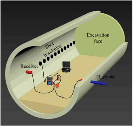
FIGURE 1. Equipment layout of TSP.

TABLE 1

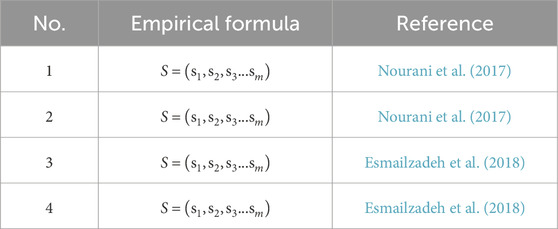
TABLE 1. Formulas denoting the relation between RMR and wave velocity in the literature.

Many research studies (Von and Ismail, 2017; Zhou et al., 2017; Li et al., 2019a; Hou et al., 2019; Lu et al., 2020) have proven that the seismic wave velocity information acquired by TSP can reflect the geological conditions in front of the tunnel face. To be specific, a portion of studies (Montalvo et al., 2015; Von and Ismail, 2017; Zhou et al., 2017; Bu et al., 2018; Li et al., 2019b; Hou et al., 2019; Shan et al., 2019; Lu et al., 2020) have revealed the link between the rock quality index and seismic wave, in particular engineering cases. For instance, Esmailzadeh et al. (2018) proposed a statistical model for RMR and TSP data. Bu et al., 2018 introduced an optimization method for classifying the advanced surrounding rock based on TSP data. Chen et al. (2017) proposed a geostatistical method for inferring RMR ahead of tunnel face excavation using dynamically exposed geological information. However, such an interpretation of refined geological data depends on the engineer’s experience, and the interpretation results are usually qualitative (Santos et al., 2015; Esmailzadeh et al., 2018). A handful of research studies have focused on the mutual link between the rock mass rating and the seismic wave velocity (Nourani et al., 2017). Moreover, considering the site characteristics, most of the models fitting the relationship between the surrounding rock quality and wave velocity have been hypothesized and optimized, which means that the estimation error of these fitting models will increase when the engineering environment changes.

Due to the ability to consider uncertainty, geostatistical approaches have been gradually adopted to estimate the RMR in different engineering projects. At present, extensive studies (Chen et al., 2018; Zhang and Zhu, 2018; Li et al., 2019b; He et al., 2020) are using the Kriging method to directly interpolate the RMR value of the whole area based on the surface exploration data and borehole data. However, these studies use limited data in the early survey stage without adopting the geological information obtained during construction. Such a phenomenon is worse in mountain tunnels as boreholes are scattered for economic reasons (Chen et al., 2017). As a result, there is a significant error in the estimation of the quality of the surrounding rock utilizing typical empirical methods. It is well-known that tunnel excavation is a dynamic process, and with the advance of the tunnel, new tunnel faces are exposed, which creates an opportunity to gather more detailed and accurate geological information. However, previous studies fail to take newly exposed geological information into account. Therefore, the main research gap this study aims to fill is how to integrate on-site data, which includes advanced geological prediction data and tunnel face data, during tunnel construction to reduce the prediction error and uncertainty of the surrounding rock.

The spatiotemporal Bayesian maximum entropy method has been successfully applied in data fusion problems in civil engineering (Li et al., 2013; Hayunga and Kolovos, 2016; Jat and Serre, 2016; Zhang et al., 2016; Gelman et al., 2017; Hu et al., 2021). However, the relation of seismic wave velocity in surrounding rock is not clear, and the BME method cannot be used to fuse the wave velocity data directly. To enhance the forecasting accuracy of rock mass quality in front of the tunnel face, it is necessary to study the prediction method that can integrate TSP wave velocity data.

Hence, in this study, the BME method integrating the TSP method is proposed to describe the relationship between newly exposed geological information and TSP data. Moreover, the observed and predicted values of RMR are compared and verified to estimate the effects of various physical parameters. Then, the performances of ordinary Kriging (OK) and BME approaches are also compared in uniform formation and the fault fracture zone to highlight the influence of the data used in RMR prediction. This study focuses on employing a dynamic Bayesian framework to quantitatively estimate RMR values in advance of the excavation face throughout tunnel construction. The main contributions of the study are summarized as follows: (1) A progressive prediction strategy for a tunnel’s surrounding rock quality was proposed. (2) The TSP-RMR statistic model was established by the Bayesian sequential update framework. (3) The uncertainty of the RMR prediction results was quantified and compared with traditional geostatistical methods. Results show that the prediction results can be improved by 15% by integrating soft data from geological interpretation.

2 Methodology

This section begins by introducing the characteristics of TSP data and explaining how to utilize TSP data for predicting the RMR value (Subsection 2.1). It then analyzes the spatial structural variability of RMR data (Subsection 2.2). Subsequently, based on the actual measurement data from the excavation face and the TSP forecast data, soft data on seismic wave velocity are obtained through Bayesian sequential updating (Subsection 2.3). Finally, the data undergo dynamic Bayesian maximum entropy fusion to yield the RMR classification results (Subsection 2.4).

2.1 RMR prediction by integrating TSP

As the tunnel excavation progresses, the geological body is exposed round by round. More accurate geological information can be obtained by a series of advanced technologies, as shown in Figure 2. The assumptions of the approach to predict RMR ahead of the excavation face include the following: (i) the geological conditions change only along the excavation direction; (ii) the RMR values obtained from the tunnel face are accurate. The design of the tunnel support structure is mainly based on the grade of the tunnel’s surrounding rock during the excavation, and it is easy to collect rock information on the tunnel face. Therefore, the above two assumptions can be accepted in the actual construction procedure of the tunnel. Assuming that $S=\left({\mathrm{s}}_1,{\mathrm{s}}_2,{\mathrm{s}}_3...{\mathrm{s}}_m\right)$ represents the excavation position, the RMR of the surrounding rock parameters at the xth position can be denoted as $RMR\left(s_x\right)$.

FIGURE 2

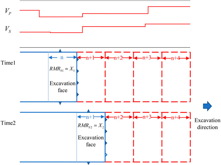
FIGURE 2. Progressive exposure characteristics of the tunnel’s surrounding rock.

For the position of ${\mathrm{S}}_{\mathrm{q}}$, $RM{R}_{\text{measured}}=RMR\left(s_1,s_2,...,s_x|x<q\right)$ represents the measured RMR value. The forecast for the geophysical parameters can be denoted as $\left(s_1,s_2,...,s_{q-1},s_q,s_{q+1},...,s_{q-n}\right)$, where $n$ is the advanced prediction detection range. Such data can be divided into two parts: $V_{measured}=V\left(s_1,s_2,...,s_{q-1}\right)$ represents the values of the measured seismic wave velocity at the given location, and $V_{prediction}=V\left(s_q,s_{q+1},...,s_{q+n}\right)$ portrays the geophysical parameters in front of the tunnel face. At this point, there is no measured RMR value in the process. The predicted value of RMR before tunnel excavation can be expressed as follows:

$RM{R}_{\text{prediction}}=RMR\left(s_q,s_{q+1},...,s_{q+n}\right).(2.1)$

Accordingly, a Bayesian stochastic analysis framework is proposed for inference RMR values in front of the tunnel face. Two types of information are used in the following prediction process: (1) RMR values measured and calculated from excavation sketches and (2) geophysical data obtained from the tunnel seismic prediction (TSP), including $V_{\mathrm{P}}$ and $V_{\mathrm{P}}/V_{\mathrm{S}}$. Depending on the uncertainty of the data, these two types of data can also be divided into hard data (measured value such as RQD) and soft data (seismic interpretation result). The conceptual workflow of the RMR prediction procedure is outlined in Figure 3.

FIGURE 3

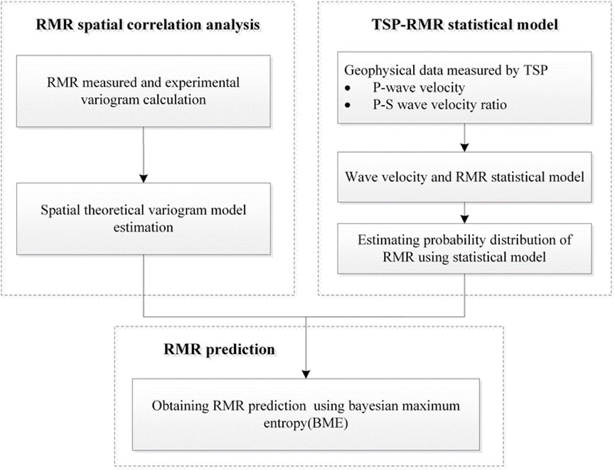
FIGURE 3. Framework of the progressive prediction strategy for the surrounding rock quality of the tunnel.

The progressive prediction strategy of RMR can be separated into the following three steps:

1) RMR spatial correlation analysis and construction of a variogram.

2) TSP-RMR statistical model based on the Bayesian updating framework.

3) RMR prediction based on the BME approach.

The RMR values were calculated, and the corresponding theoretical variogram model was fitted accordingly. The range of the variogram can be used to determine the locations of the data points used in the prediction. All steps are described in the following sections in detail.

2.2 RMR spatial correlation analysis and the built of the variogram

In the hypothesis of the geostatistical theory, adjacent geological data show similar properties (Chen et al., 2017); therefore, RMR data from similar areas can be used to forecast the quality of the surrounding rock at unknown points. This spatial correlation of the geological condition of the excavation face at different positions can be expressed by a variogram. The variogram is defined as the expectation of the variance of regional variables as follows:

$2\gamma \left(x,h\right)=\text{var}\left[Z\left(x\right)-Z\left(x+h\right)\right]={\left\{E\left[Z\left(x\right)-Z\left(x+h\right)\right]\right\}}^2,(2.2)$

where Z represents a stationary random function, including the known mean $m$ and variance ${\sigma }^2$, which is independent of location; therefore, $m\left(x\right)=m$ and ${\sigma }^2\left(x\right)={\sigma }^2$ for all places $x$ in the research region. The RMR of the tunnel excavation surface can be treated as a one-dimensional variable along the tunnel axis. The spatial correlation is obtained by calculating the experiment variogram and fitted using theoretical variogram models (i.e., spherical model, exponential model, and Gaussian model).

Due to that, the peculiarities of the geological data are gradually revealed during tunnel excavation, and a series of observation data are utilized to build a variogram model for each prediction point. The range and sill are two essential components in the variogram function. The hard data beyond the range will not be included in the prediction.

2.3 TSP-RMR statistical model based on the Bayesian updating framework

2.3.1 Dynamic Bayesian framework

Assume that the relationship between RMR and wave velocity can be shown by.

$f\left(x\right)={\mathbf{x}}^{\mathrm{T}}\mathbf{w},\mathbf{y}=a\mathbf{x}+b+\mathbf{\epsilon },(2.3)$

$a\sim N\left({\mu }_a,{\sigma }_a^2\right),b\sim N\left({\mu }_b,{\sigma }_b^2\right),\mathbf{\epsilon }\sim N\left(0,{\sigma }_t^2\right),(2.4)$

where $x$ is the wave velocity data ($V_{\mathrm{P}}$ or $V_{\mathrm{P}}/V_{\mathrm{S}}$), $y$ shows the observed performance, $w=\left\{a,b\right\}$ are the regression parameters, and $\epsilon$ represents the uncertainty variable, describing the observation error. The model parameter $w$ is assumed to be a normal or lognormal distribution. The Gaussian error with zero mean and variance ${\sigma }_t^2$ is used to represent the observation error $\epsilon$.

The Bayesian method can use observation samples to update model parameters. The posterior distribution of model parameter $\theta =\left\{\mathbf{w},\epsilon \right\}$ can be obtained by integrating prior information and the likelihood function from the observation values, which is expressed in Eq. 2.5.

$P\left(\theta |\mathbf{x},\mathbf{y}\right)=\frac{P\left(\mathbf{y}|\mathbf{x},\theta \right)P\left(\theta \right)}{\int P\left(\mathbf{y}|\mathbf{x},\theta \right)P\left(\theta \right)\mathrm{d}\theta }=kP\left(\mathbf{y}|\mathbf{x},\theta \right)P\left(\theta \right),(2.5)$

where $k$ is a normalization constant to ensure that the posterior probability density function (PDF) $P\left(\theta |x,y\right)$ is valid. $P\left(\theta \right)$ is the prior PDF of parameters, which can be obtained through previous engineering information and expert experience. $P\left(y|x,\theta \right)$ is the likelihood function, reflecting the observation conditional probability of y. $P\left(\theta |x,y\right)$ represents the posterior PDF.

Figure 4 demonstrates the basic principle of the Bayesian updating framework, and $P\left(\theta \right)$ is updated in each step of the prediction. Its implementation can be summarized as considering the posterior distribution of the parameters predicted in the previous step as the prior distribution of the parameters updated in the next step. According to the Bayesian theorem, the posterior distribution of the stage is expressed as follows:

$P\left(\theta |{\text{DATA}}_{\mathrm{I}}\right)=K_{I}P\left({\text{DATA}}_I|\theta \right)P\left(\theta \right).(2.6)$

FIGURE 4

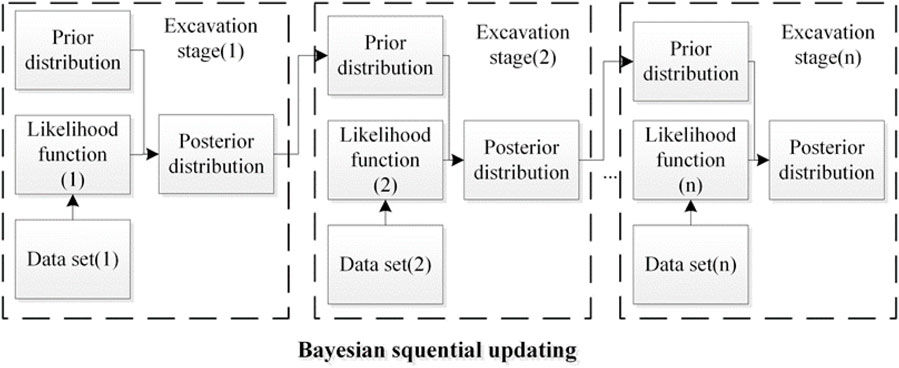
FIGURE 4. Processing of soft data based on Bayesian sequential updating.

Due to the complexity of the likelihood function and integral term, an analytic representation of posterior distribution is difficult to obtain directly. Thus, it is gained through the numerical integration method or sampling method. In this paper, the sampling method based on the Markov chain Monte Carlo (MCMC) simulation is suitable for deriving the posterior PDF. MCMC is a numerical method to generate random sample data to obtain distribution parameters. The Gibbs sampling algorithm is used in MCMC to generate the equivalent sample.

Tunnel excavation is a process in which the measured data gradually increase. The measured RMR data and wave velocity information gradually revealed can be used as a dataset to calculate the likelihood function of the new stage. Therefore, in the Bayesian sequence updating framework, each excavation process of the tunnel can be regarded as a new updating stage.

2.3.2 Prior PDF parameter setting

The prior distribution of the parameters is determined by the posterior distribution of the previous prediction results. The model parameter $w$ is assumed to be a normal distribution with a mean of $u_w$ and a variance of ${\sigma }_w^2$.

$\mathbf{w}\sim N\left({\mathbf{u}}_{\mathbf{w}},{\mathbf{\sigma }}_{\mathbf{w}}^{\mathbf{2}}\right).(2.7)$

In the first step of prediction, the prior information about the model can be determined according to the engineering experience. Assuming that the prior information is ${\mu }_a={\mu }_b=0$, ${\sigma }_a^2={\sigma }_b^2={10}^4$ represents that model parameters can be specified in a certain range before the observation data are obtained.

It should also be noted that the observation error is very important in the estimate of the likelihood function. The observation error ($\epsilon$) is assumed to be a normal distribution with zero mean and a standard deviation of 1.0, based on the experience in Yunnan and the reports in the literature about measured RMR based on photography.

2.3.3 Soft data probability distribution calculation

After the posterior distribution of the model parameters is obtained, the RMR probability distribution from wave velocity inversion can be calculated by Eq. 2.8:

$P\left(\mathbf{y}|\mathbf{x},\text{DATA}\right)={\displaystyle \underset{\theta }{\int }}P\left(\mathbf{y},\theta |\mathbf{x},\text{DATA}\right)\mathrm{d}\theta .(2.8)$

In this study, the model parameters $\mathbf{w}$ and observation errors $\epsilon$ follow the assumption of normal distribution and are independent of each other. Therefore, the RMR soft data obtained by wave velocity fitting also conform to normal distribution.

2.4 Bayesian maximum entropy (BME) approach

The overall framework of the Bayesian maximum entropy approach is shown in Figure 5. The Bayesian maximum entropy approach can integrate physical knowledge from different sources, uncertainty information, and statistical moments into a spatiotemporal random field (Christakos, 1990). The interpretation results of RMR with TSP based on Bayesian dynamic updating are substituted into the Bayesian maximum entropy framework as soft data, and finally, the predicted RMR value at the unexcavated position beyond the tunnel excavation face can be obtained.

FIGURE 5

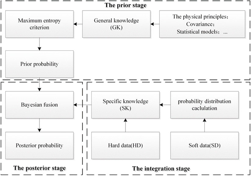
FIGURE 5. Framework of the Bayesian maximum entropy approach.

Suppose that there are a total of m data points in the sampling space, which contain $h$ hard data and $m-h$ soft data. Accordingly, the hard data are represented as $x_{\text{hard}}=\left(x_1,...,x_h\right)$, and the soft data are represented as $x_{\text{soft}}=\left(x_{h+1},...,x_{h+m}\right)$. The BME method is used to predict the point values and calculate posterior PDF based on the estimated values from the expected value. The posterior probability of the prediction is calculated as follows:

$f\left(x_k|x_1,x_2,...,x_m\right)=\frac{f\left(x_k|x_1,x_2,...,x_m,x_k\right)}{f\left(x_1,x_2,...,x_m\right)},(2.9)$

$\overline{x_{km}}=\int x_{k}f\left(x_k\right)d{x}_k.(2.10)$

The basic flow of BME (Figure 5) includes three basic steps:

1) The prior stage: at this stage, the basic knowledge (BK) is integrated with the prior distribution, which is given using the maximum entropy criterion. Generally, the prior PDF of maximum entropy can be calculated by the Lagrange optimization operator, which can be calculated as follows:

$f_G\left(x\right)=K^{-1}\exp \left[{\displaystyle \sum _{\alpha =1}^N}{\mu }_{\alpha }{g}_{\alpha }\left(x\right)\right],(2.11)$

where $f_G\left(x\right)$ is the prior probability distribution under the maximum-entropy condition. $g_{\alpha }$ is a known function between the random variables. ${\mu }_{\alpha }$ is the Lagrange multiplier. $N$ represents the number of constraints, and K represents the regularization parameter.

2) The integration stage: this phase combines the hard and soft data to form a specific knowledge base (SK). In this paper, the hard data come from the measured RMR on the tunnel face, while the soft data come from the wave velocity data obtained by TSP advance prediction and from the fitting model of the surrounding rock parameters.

3) The posterior stage: at this stage, GK and SK are integrated. The prior PDF obtained in the first step and the specific knowledge base in the second step are processed by the Bayes rule to solve the posterior PDF. Finally, the mathematical expectation is obtained as the predicted value of the point to be estimated.

3 Case study of the Laoying tunnel

3.1 Project overview

A case study was performed to validate the RMR prediction method proposed in this study. The Laoying rock tunnel is a separate rock tunnel constructed by the drilling and blasting method in Baoshan, Yunnan, China (see Figure 6). The study area is located between the mileages K12 + 320 and K11 + 320, with a total length of 1,115 m. The maximum buried depth of the Laoying tunnel is approximately 1,264 m. The underground space traversed by the project mainly contains rock layers such as sandstone and limestone, and the preliminary survey reveals five large faults along the tunnel axis.

FIGURE 6

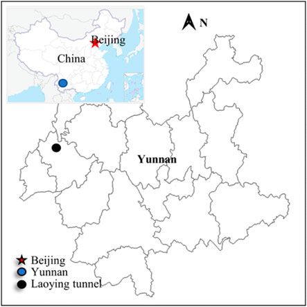
FIGURE 6. Location of the Laoying tunnel in China.

3.2 Data collection

A series of photogrammetry and field tests were performed to obtain the value of RMR on the tunnel face as hard data. The new tunnel face, which was exposed by tunnel drilling and blasting, created opportunities for engineers to inspect the rock masses. In this study, the surrounding rock evaluation parameters in RMR are collected herein. As shown in Figure7, the integrity index (RQD value, joint spacing, and joint condition) of the tunnel face was obtained by the photogrammetry-based mapping technique (Li et al., 2016), and the UCS of the rock mass can be obtained through the rebound tests of the rock mass. Ground water (GW) data are obtained by field observation. A part of the measured RMR values of the tunnel faces is given in Table 2.

FIGURE 7

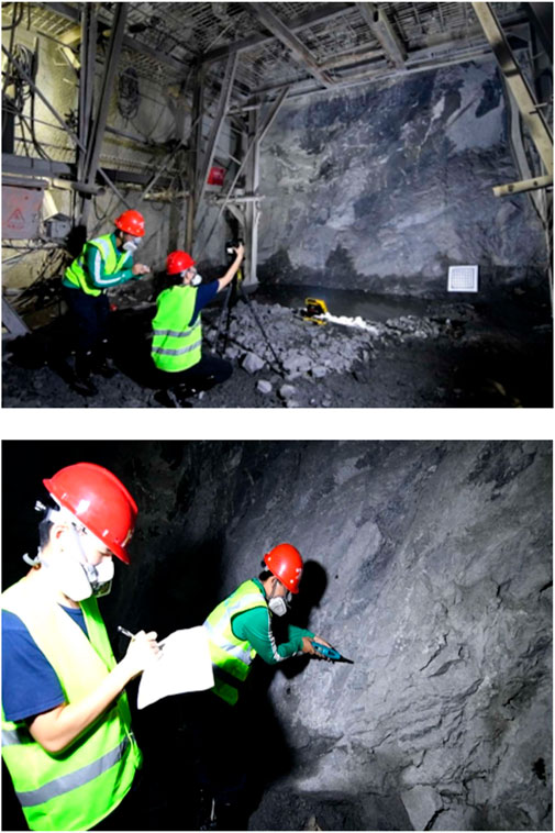
FIGURE 7. Data measured from the tunnel face.

TABLE 2

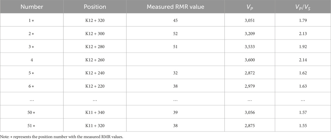
TABLE 2. Measured RMR values on the tunnel faces.

During tunnel construction, a total of nine TSP tests were conducted in the designated location from K11 + 320 to K12 + 320 (see Figure 8). Each TSP seismic wave forecast can observe the seismic p-wave and s-wave velocities in the rock mass within 100–120 m in front of the tunnel face. By analyzing the wave velocity inversion results of the nine TSP predictions, $V_{\mathrm{P}}$ and $V_{\mathrm{S}}$ of the rock mass were collected every 20 m from the position of K12 + 320. In the selected study area, the tunnel passes through a fault zone, which is approximately located between K11 + 470 and K11 + 320, according to the preliminary geological survey.

FIGURE 8

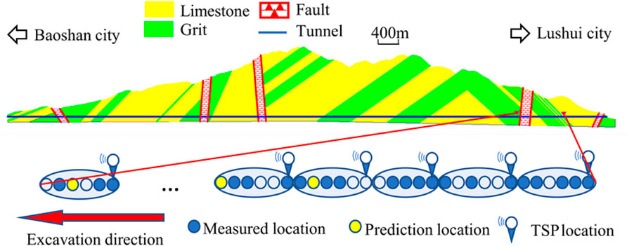
FIGURE 8. Excavation profile of the Laoying tunnel.

4 Results and discussion

4.1 Probabilistic characteristics of RMR with wave velocity fitting

Figure 9 displays the RMR values of K11 + 360, as interpreted by $V_P$ and $V_S/V_S$, respectively. A total of 10,000 equivalent samples of the statistic parameters were generated using the proposed Bayesian sequential updating approach to ensure that the MCMC method achieves a stable convergence state. The RMR value at K11 + 360 was interpreted when the tunnel was excavated to K11 + 880, K11 + 740, K11 + 480, and K11 + 340, referring to excavation stages 1, 2, 3, and 4, respectively. Figure 10 displays the MCMC equivalent sample and statistical diagram of the parameter at K11 + 360 under the conditions of the first excavation stage. Therefore, as the excavation continues, the available measured data gradually increase, and the predicted variance decreases. For each prediction point, soft data select the interpretation results of the stage in which the excavation position is closest to the prediction point. In excavation stage 4, where the excavation faces reach K11 + 340, when $V_P$ and $V_P/V_S$ are used to interpret RMR, the mean and variance of K11 + 360 interpretation data are (39.7032, 3.509) and (38.5254, 3.387), respectively. These two values are used as soft data at K11 + 360, when the excavation position is closest to the prediction point as many measured data can be employed. The soft data forecasting the rest of K11 + 360 also employed MCMC statistics from this construction phase. Correspondingly, when predicting K11 + 900, K11 + 760, and K11 + 480, the parameters of the excavation stage 1, stage 2, and stage 3 are used, respectively. In order to increase the prediction accuracy, all available hard data are used in this process.

FIGURE 9

FIGURE 9. RMR interpretation values in different excavation stages at K11 + 360.

FIGURE 10

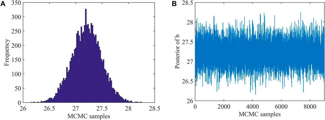
FIGURE 10. TSP and RMR statistical parameters in excavation stage 1; (A) equivalent sample frequency distribution; (B) equivalent samples based on MCMC.

4.2 Hard data spatial variability

Figure 11 shows the results of the variogram calculation by fitting the positions of the four predicted points to the spherical theoretical variogram. The variogram function reflects the spatial variability of the surrounding rock parameters. The data range and sill are listed in Table 3, and the data points outside the range will no longer participate in the prediction.

FIGURE 11

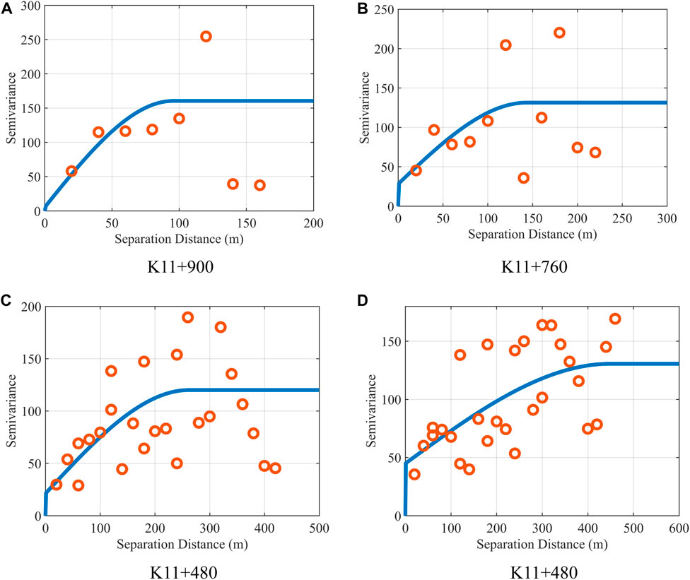
FIGURE 11. Variogram function fitting: (A) K11 + 900 variogram model, (B) K11 + 760 variogram model, (C) K11 + 480 variogram model, and (D) K11 + 360 variogram model.

TABLE 3

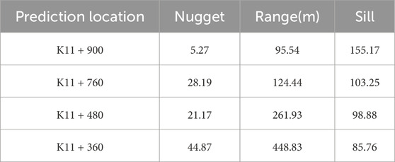
TABLE 3. Cross-validation criteria for different excavation stages ($V_P$ as soft data).

The variogram function changes as the measurement data increase, which can be seen from the fitting results. The range grows with more measured data, indicating that more hard data need to be included to yield more accurate results in the limited area. However, the nugget increases with a larger sample size, proving that the influence of the aggregate error of the sampling measurement increases accordingly. The prediction deviation caused by the internal randomness of the surrounding rock mass parameters will be more evident in the regions that do not conform to the hypothesis of second-moment stability, such as the fault fracture zone. Therefore, it is necessary to perform advanced geological prediction to improve the prediction accuracy.

4.3 Exploratory spatial data analysis

Figure 12 shows the data location for the prediction of mileage K11 + 760. A total of 17 hard data and 22 soft data were collected for advanced geological prediction. The prediction point lies between the measurement position of the hard data and soft data. The measured values of RMR ranged from 22 to 57, the mean is 40.8, and the standard deviation is 9.69. Figure 13 also illustrates the frequency distribution histogram of RMR. The Shapiro–Wilk method was used to test the normality of the RMR data distribution. The results show that the measured values of RMR do not reject the normal distribution at the significance level of 5%. The BME method requires the hard data used to follow the normal distribution, so the hard data used for the other predicted positions are also tested for the normal distribution.

FIGURE 12

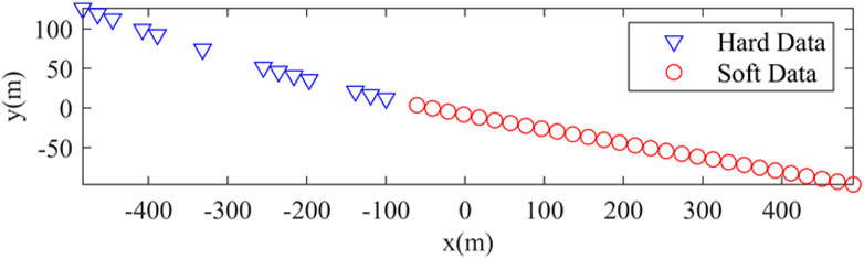
FIGURE 12. K11 + 900 soft data and hard data location distribution.

FIGURE 13

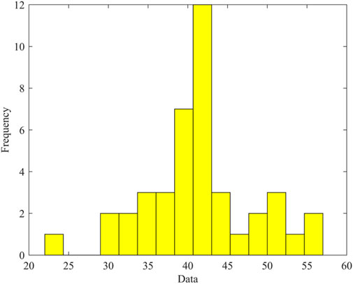
FIGURE 13. Frequency distribution histogram of measured RMR.

4.4 Comparison and analysis of the prediction results

4.4.1 Comparison and verification with the measure values

The prediction results of different excavation stages are summarized in Figure 14, where a prediction that considers $V_P$ as soft data and a prediction that considers $V_P/V_S$ as soft data are presented separately. The performance metrics, maximum deviation (MD), mean error (ME), and root mean squared error (RMSE) are used for evaluating the prediction accuracy. As shown in Table 4 and Table 5, these evaluation parameters should be as small as possible. The predicted accuracy increases with the amount of hard data. At excavation stage 1 (from excavation to K11 + 900), when the number of the measured data is 12, the RMSE of the predicted result is 5.11. At excavation stage 4, when the number of the measured data increased to 30, the RMSE of predicted result is 1.65, which causes a smaller RMR prediction uncertainty compared with that of excavation stage 1.

FIGURE 14

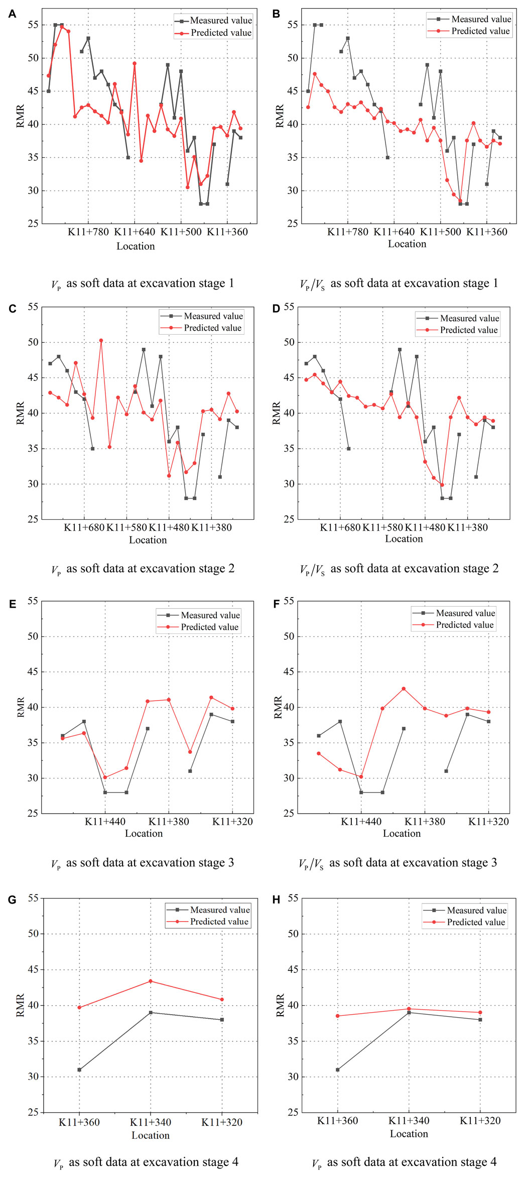
FIGURE 14. BME prediction result at different excavation stages ((A, B): excavation stage 1; (C, D): excavation stage 2; (E, F): excavation stage 3; (G, H): excavation stage 4).

TABLE 4

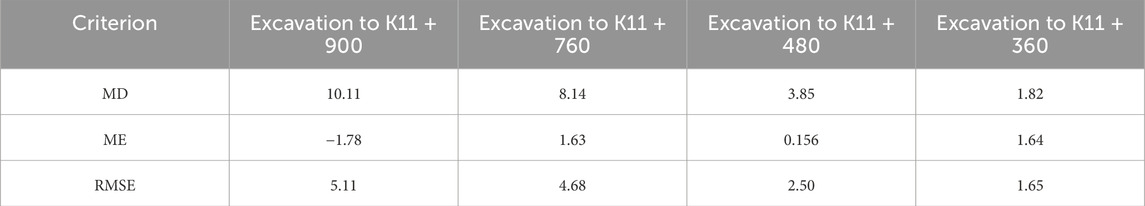
TABLE 4. Cross-validation criteria for different excavation stages ($V_P$ as soft data).

TABLE 5

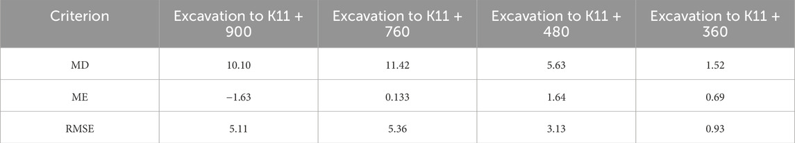
TABLE 5. Cross-validation criteria for different excavation stages ($V_P/V_S$ as soft data).

Moreover, as illustrated in Table 4 and Table 5, the RMR prediction results using $V_P$ and $V_P/V_S$ have almost similar estimation accuracies in terms of MD, ME, and RMSE values. However, from the perspective of the discretization and volatility of the prediction results, the volatility of the prediction results is smaller when $V_P/V_S$ is used as soft data. For example, when the construction reaches K11 + 900, the sample variances of the two prediction methods are 5.94 and 3.32, respectively.

4.4.2 Comparison and verification with the measure values

For the Kriging method (Hayunga and Kolovos, 2016; Zhang et al., 2016; Gelman et al., 2017; He and Kolovos, 2018), the measured value of RMR for each excavated surface is taken as sample points, and the variogram function in Figure 11 is used for the fitting prediction. In the Kriging prediction framework, only hard data from the excavation face are included in the prediction. The RMR prediction uncertainty can be quantified by considering the model uncertainty and spatial variability. The estimation with the 68% confidence interval of RMR can be represented as follows: $\left[{\mu }_{\text{lower}}-\sigma ,{\mu }_{upper}-\sigma \right]$. As illustrated in Figure 15, the blue line represents the actual measured RMR at the excavated positions, and the purple and red lines represent the predicted RMR value using the OK and BME methods, respectively.

FIGURE 15

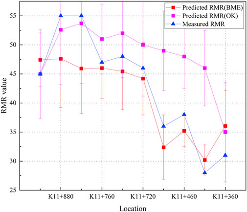
FIGURE 15. Result comparison of Kriging and BME methods.

As is shown in Figure 15, the BME-based approach shows a smaller prediction error than the OK-based method, and such a phenomenon is more obvious in the fault area. According to the tunnel preliminary geological survey, the area between K11 + 470 and K11 + 320 is located in a fault. It is tough to forecast the accuracy of drastic changes in geological conditions in bad geological sections such as faults. Therefore, it is necessary to apply an advanced geological prediction to assist in predicting the geological conditions. Table 6 indicates the relative errors of the three prediction approaches in the formation of relatively uniform sections, such as the K11 + 900 and K11 + 760 forecast points. The relative errors of the three methods are reasonably minor, and the relative errors of the predicted results are less than 15%. However, the relative error predicted by the Kriging method is up to 30% when the local layer varies significantly in fault fracture zones, such as at K11 + 480 and K11 + 360. At this time, the prediction results have a larger deviation, which proves the previous hypothesis. It is difficult to capture large strata changes using traditional Kriging methods. In comparison, the two BME prediction results, which combine the wave velocity of the surrounding rock in advance, have better prediction results at the fault layer. Two performance metrics, ME and RMSE, are used to assess the overall predictive accuracy. The ME should approach zero. The RMSE shows the difference between the predicted and the measured values, which needs to be as small as possible. As shown in Table 7, RMSE for BME ($V_P$) and BME ($V_P/V_S$) are 2.91 and 2.35, respectively. Therefore, $V_P/V_S$ information as soft data in the research area has a relatively higher accuracy.

TABLE 6

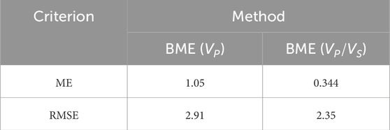
TABLE 6. Relative errors of different prediction methods.

TABLE 7

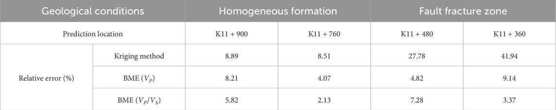
TABLE 7. Validation criteria for two BME prediction strategies.

5 Conclusion

This paper proposes a statistical method based on the Bayesian maximum entropy framework, which uses geological information on the tunnel face and TSP geological prediction to quantitatively infer the RMR value of the unexcavated rock mass. The proposed method is applied in the Laoying rock tunnel in Yunnan, China. The RMR values at each excavation position of the tunnel are obtained by photogrammetry and other complementary methods. Additionally, the variances of different measured data are calculated.

Second, two parameters, the s-wave velocity and p-wave velocity ratio of surrounding rock, were selected to fit the RMR of the surrounding rock, and the least square fitting interval of the 95% confidence level was selected as the wave velocity measurement point to participate in the Bayesian maximum entropy prediction.

Finally, the Bayesian maximum entropy and traditional Kriging methods are used to analyze the prediction results of the normal uniform formation and the fault fracture zone in the study area. Meanwhile, the prediction results using p-wave velocity and p-wave velocity ratio as soft data are compared. The results show that the Bayesian maximum entropy can integrate the advanced geological prediction data, and the prediction accuracy is higher in the sections where the geological conditions change significantly, such as the fault fracture zone. In comparison, $V_P/V_S$ information as soft data has a relatively higher accuracy.

The results indicate that the fusion of soft data and geological interpretation can make the prediction of RMR more accurate. The relative error of the method is less than 15% at the selected prediction points compared with that of the traditional Kriging method. This method shows significant potential for estimating RMR values ahead of tunnel excavation with advanced geological forecast data.

Data availability statement

The raw data supporting the conclusion of this article will be made available by the authors, without undue reservation.

Author contributions

XL: data curation, funding acquisition, resources, supervision, writing–original draft, and writing–review and editing. ZC: methodology and writing–original draft. LT: formal analysis, methodology, and writing–review and editing. CC: writing–review and editing. TL: methodology and writing–review and editing. JL: writing–review and editing. YL: data curation and writing–review and editing. YR: funding acquisition, supervision, validation, and writing–review and editing.

Funding

The author(s) declare financial support was received for the research, authorship, and/or publication of this article. This work was financially supported by the National Natural Science Foundation of China (grant number: U1934212). The authors would like to thank the financial support.

Conflict of interest

The authors declare that the research was conducted in the absence of any commercial or financial relationships that could be construed as a potential conflict of interest.

Publisher’s note

All claims expressed in this article are solely those of the authors and do not necessarily represent those of their affiliated organizations, or those of the publisher, the editors, and the reviewers. Any product that may be evaluated in this article, or claim that may be made by its manufacturer, is not guaranteed or endorsed by the publisher.

References

Bieniawski, Z. (1973). Engineering classification of jointed rock masses. Civ. Eng. 15, 334–345.

Google Scholar

Bu, L., Li, S. C., Shi, S. S., Xie, X. K., Li, L. P., Zhou, Z. Q., et al. (2018). A new advance classification method for surrounding rock in tunnels based on the set-pair analysis and tunnel seismic prediction system. Geotechnical Geol. Eng. 36, 2403–2413. doi:10.1007/s10706-018-0471-5

CrossRef Full Text | Google Scholar

Chen, G. X., Zhu, J., Qiang, M., and Gong, W. (2018). Three-dimensional site characterization with borehole data - a case study of Suzhou area. Eng. Geol. 234, 65–82. doi:10.1016/j.enggeo.2017.12.019

CrossRef Full Text | Google Scholar

Chen, J., Li, X., Zhu, H., and Rubin, Y. (2017). Geostatistical method for inferring RMR ahead of tunnel face excavation using dynamically exposed geological information. Eng. Geol. 228, 214–223. doi:10.1016/j.enggeo.2017.08.004

CrossRef Full Text | Google Scholar

Christakos, G. (1990). A Bayesian maximum-entropy view to the spatial estimation problem. Eng. Geol. 22, 763–777. doi:10.1007/bf00890661

CrossRef Full Text | Google Scholar

Esmailzadeh, A., Mikaeil, R., Shafei, E., and Sadegheslam, G. (2018). Prediction of rock mass rating using TSP method and statistical analysis in Semnan Rooziyeh spring conveyance tunnel. Tunneling Undergr. Space Technol. 79, 224–230. doi:10.1016/j.tust.2018.05.001

CrossRef Full Text | Google Scholar

Gelman, A., Simpson, D., and Betancourt, M. (2017). The prior can often only Be understood in the context of the likelihood. Entropy 19, 555–625. doi:10.3390/e19100555

CrossRef Full Text | Google Scholar

Hayunga, D. K., and Kolovos, A. (2016). Geostatistical space-time mapping of house prices using Bayesian maximum entropy. Int. J. Geogr. Inf. Sci. 30, 2339–2354. doi:10.1080/13658816.2016.1165820

CrossRef Full Text | Google Scholar

He, H. H., He, J., Xiao, J. Z., Zhou, Y., and Liu, Y. (2020). 3D geological modeling and engineering properties of shallow superficial deposits: a case study in Beijing, China. Tunn. Undergr. Space Technol. 100, 103390–103418. doi:10.1016/j.tust.2020.103390

CrossRef Full Text | Google Scholar

He, J., and Kolovos, A. (2018). Bayesian maximum entropy approach and its applications: a review. Stoch. Environ. Res. Risk Assess. 32, 859–877. doi:10.1007/s00477-017-1419-7

CrossRef Full Text | Google Scholar

Hoek, E., and Brown, E. T. (1997). Practical estimates of rock mass strength. International Journal of Rock Mechanics and Mining Sciences 34 (8), 1165–1186.

CrossRef Full Text | Google Scholar

Hou, F., Xie, X., Shi, S., Song, S., Bu, L., Li, L., et al. (2019). Dynamic optimization classification model for submarine tunnel surrounding rocks and its application in engineering. J. Coast. Res. 15, 311–315. doi:10.2112/si94-064.1

CrossRef Full Text | Google Scholar

Hu, B., Ning, P., Li, Y., Xu, C., Christakos, G., and Wang, J. (2021). Space-time disease mapping by combining Bayesian maximum entropy and Kalman filter: the BME-Kalman approach. Int. J. Geogr. Inf. Sci. 35, 466–489. doi:10.1080/13658816.2020.1795177

CrossRef Full Text | Google Scholar

Jat, P., and Serre, M. (2016). Bayesian Maximum Entropy space/time estimation of surface water chloride in Maryland using river distances. Environ. Pollut. 219, 1148–1155. doi:10.1016/j.envpol.2016.09.020

PubMed Abstract | CrossRef Full Text | Google Scholar

Li, J., Zhang, H., and He, J. (2019a). Application of integrated geophysical methods to advanced prediction of a tunnel in a limestone area. Geol. Explor. 55, 1452–1462.

Google Scholar

Li, N., Song, X. L., Li, C., Xiao, K., Li, S., and Chen, H. (2019b). 3D geological modeling for mineral system approach to GIS-based prospectivity analysis: case study of an MVT Pb–Zn deposit. Nat. Resour. Res. 28, 995–1019. doi:10.1007/s11053-018-9429-9

CrossRef Full Text | Google Scholar

Li, X., Chen, J., and Zhu, H. (2016). A new method for automated discontinuity trace mapping on rock mass 3D surface model. Comput. Geosciences 89, 118–131. doi:10.1016/j.cageo.2015.12.010

CrossRef Full Text | Google Scholar

Li, X., Li, P., and Zhu, H. (2013). Coal seam surface modeling and updating with multi-source data integration using Bayesian Geostatistics. Eng. Geol. 164, 208–221. doi:10.1016/j.enggeo.2013.07.009

CrossRef Full Text | Google Scholar

Lu, Q., Zhao, B., and Pan, S. (2020). Classification of tunnel surrounding rock based on TSP system and PCA-bayes discriminant method. Chin. J. Undergr. Space Eng. 16, 80–86.

Google Scholar

Montalvo, D., Mclaughlin, M., and Degryse, F. (2015). Efficacy of hydroxyapatite nanoparticles as phosphorus fertilizer in andisols and oxisols. Soil Sci. Soc. Am. J. 79, 551–558. doi:10.2136/sssaj2014.09.0373

CrossRef Full Text | Google Scholar

Niedbalski, Z., Małkowski, P., and Majcherczyk, T. (2018). Application of the NATM method in the road tunneling works in difficult geological conditions–The Carpathian flysch. Tunn. Undergr. Space Technol. 74, 41–59. doi:10.1016/j.tust.2018.01.003

CrossRef Full Text | Google Scholar

Nourani, M., Moghadder, M. T., and Safari, M. (2017). Classification and assessment of rock mass parameters in Choghart iron mine using P-wave velocity. J. Rock Mech. Geotechnical Eng. 9, 318–328. doi:10.1016/j.jrmge.2016.11.006

CrossRef Full Text | Google Scholar

Santos, V., Da, S., and Graca, M. B. (2015). Prediction of RMR ahead excavation front in D&B tunnelling. Eng. Geol. Soc. Territ. 6, 415–419.

CrossRef Full Text | Google Scholar

Shan, S. W., Lam, T. C., and Stamer, W. D. (2019). The effects of a Rho-associated protein kinase (ROCK) inhibitor (Y39983) on human trabecular meshwork cells - a morphological and proteomic study. Investigative Ophthalmol. Vis. Sci. 60, 9–12.

Google Scholar

Von, W., and Ismail, M. (2017). “Evaluation of tunnel seismic prediction (TSP) result using the Japanese highway rock mass classification system for pahang-selangor raw water transfer tunnel,” in Proceedings of the International Conference of Global Network for Innovative Technology and Awam International Conference in Civil Engineering, Penang, Malaysia, August 8–9, 2017.

CrossRef Full Text | Google Scholar

Zhang, F., Zhong, S., Yang, Z., Sun, C., Wang, C. L., and Huang, Q. Y. (2016). Spatial estimation of losses attributable to meteorological disasters in a specific area (105.0°e–115.0°E, 25°N–35°N) using bayesian maximum entropy and partial least squares regression. Adv. Meteorology 2016, 1–16. doi:10.1155/2016/1547526

CrossRef Full Text | Google Scholar

Zhang, Q., and Zhu, H. (2018). Collaborative 3D geological modeling analysis based on multi-source data standard. Eng. Geol. 246, 233–244. doi:10.1016/j.enggeo.2018.10.001

CrossRef Full Text | Google Scholar

Zhou, Z., Li, S., and Li, L. (2017). Classification method of rock mass quality and its engineering application. J. Central South Univ. Sci. Technol. 48, 1049–1056.

Google Scholar