An inversion method for imaging near-wellbore thin beds slowness based on array acoustic logging data

As a practical approach to reflecting the properties of the formation, the slowness of near-wellbore formation is of great significance to geophysical exploration, which can be used to evaluate rock brittleness, wellbore stability, fracturing effect, and invasion depth. Although traditional slowness imaging methods perform well in areas where the thickness of the heterogeneous formation is greater than the length of the receiver array of the logging instrument, they may fail when encountering thin beds. The thin beds’ axial thickness, radial invasion depth, and radial slowness are challenging to identify, resulting in obtaining an average slowness value without longitudinal resolution. This paper proposes a thin beds slowness imaging inversion method that can effectively invert the axial thickness, radial invasion thicknesses, and radial slowness variations of thin beds with higher axial resolution compared to traditional methods. The new method adaptively extracts slowness sequences with different radial depths by combining receivers with different source distances. It obtains their corresponding radial thicknesses through ray theory, which does not depend on the arrival times of the first wave. This method is sensitive to thin beds, and the axis thickness of thin beds can be estimated by the change of radial slowness sequence and the combined source distance length. Combining the results at different depths allows a slowness image of the thin beds near-wellbore to be directly obtained. The effectiveness and accuracy of the proposed method are verified by synthetic data and field data.

1 Introduction

In geophysical exploration, the array acoustic logging technique effectively characterizes the formation properties around the well. The technique excites the sound source every 0.1524 m along the shaft well axis and uses a receiving array to record the waveforms. The compressional and shear wave slowness at each depth point is obtained by analyzing the arrival time of the waveforms. However, the formation properties near-wellbore are often altered by stress conditions, fluid invasion, and mechanical damage resulting from drilling (Baker and Winbow, 1988), which usually manifests as variations of slowness in axial and radial formations (Pistre et al., 2005). In addition, the thin beds, due to their small thickness, often display significant contrasts in slowness between layers (Xu et al., 1995). The axial and radial variations of the slowness require a higher resolution characterization of slowness distributions at each depth point. The distribution of slowness is of great importance for assessing borehole stability (Winkler, 2005), estimating formation stress (Sayers et al., 2008), optimising reservoir production (Tang et al., 2016), and guiding well drilling completion (Sinha et al., 2005). Several methods have been proposed to perform the inversion of slowness images. Some scholars (Hornby, 1993; Zeroug et al., 2006) attempted to establish the tomographic reconstruction based on the simultaneous iterative reconstruction technique (SIRT) and ray tracing theory (Dines and Lytle, 1979). Liu et al. (2021) developed a stepwise inversion method to solve the first arrival times dependency. Sinha et al. (2006) proposed to use the technique using B-G theory (Backus et al., 1970) inversion of the measured cross-dipole dispersions to map the average slowness distribution at the expense of radial resolution. Tang and Patterson (2010) adopted a new constraint to solve the non-unique problem of estimating the radial variation from dispersion data. Moreover, Ma et al. (2013) used the perturbation method and B-G theory to map the radial alteration of formation shear wave slowness. Although these methods perform well in slowness imaging of radial heterogeneous formations in the entire well section, they will decrease the accuracy of the slowness imaging due to spatial averaging caused by the sonic receiver array across thin beds (Huang and Torres-Verdin, 2016). The slowness results are the average contribution of each formation in the exploration area. The contribution of the thin beds cannot be identified. So, obtaining the specific location of the thin bed is impossible, and the actual slowness of each formation cannot be known from the slowness results (Lei et al., 2019).

This study aims to develop an automatic method to invert the near-wellbore thin bed’s slowness from the monopole acoustic logs. Different from traditional slowness inversion methods, this method can effectively identify the axial position, axial thickness, radial invasion depth, and radial slowness of thin beds by processing the data of conventional array acoustic logging instruments, which completely solves the limitation that traditional methods cannot quantitative characterization of the thin beds. In the new method, we first focus on the stable method of extracting slowness. We accumulate the results of the slowness time coherence (STC) (Kimball and Marzetta, 1984) method in the time domain and determine the position of the maximum correlation value by the crest. The advantage of this approach is that it solves the problem of the slowness extraction method failing when the waveform correlation is poor and makes it stable and fast automatic acquisition in various situations. In characterising thin bed properties, different from the conventional slowness extraction, we improve axial and radial resolutions by recombining array acoustic log data from receivers to obtain multiple slowness sequences at the same depth point. Slowness sequence can qualitatively characterise the homogeneous formation, heterogeneous formation and thin bed. The thin bed’s axial position, axial thickness, and radial slowness distribution can be further quantitatively characterised by ray theory. Finally, we obtain the near-wellbore thin beds slowness image using inverse-distance weighting (IDW) interpolation on the discrete radial slowness distribution information.

We use the finite difference time domain (FDTD) method (Cheng et al., 1995) to calculate the resultant waveform under the excitation of a unipolar source on the well axis. This inversion method then processes these signals to estimate the axial position, axial thickness and slowness distribution of near-wellbore thin beds, and the inversion results are close to the initial model. We also apply this method to a well in western China, and the inversion results correctly indicate the depth of the thin beds. Both the inversion results of the synthetic and field examples demonstrate the accuracy of the thin beds’ slowness imaging inversion method. The significant advantage of the new method is that it improves the axial resolution of slowness imaging and can effectively indicate the exact position and slowness distribution of multiple thin beds. Figure 1A shows the workflow of our proposed method.

FIGURE 1

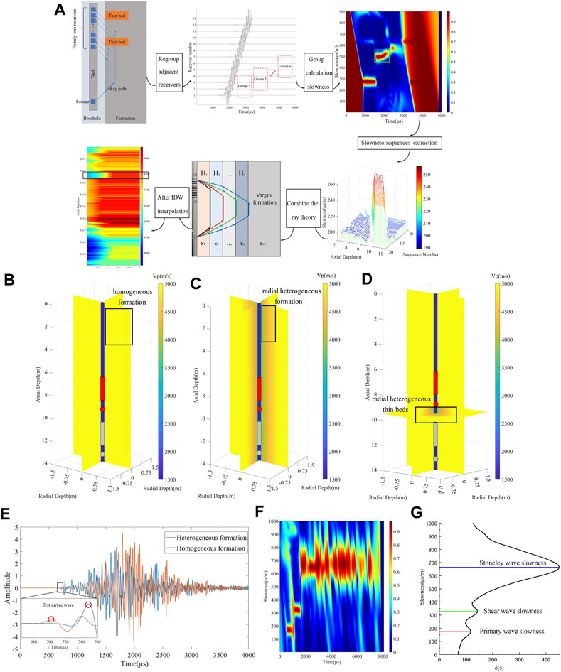
FIGURE 1. Introduction of the thin beds slowness inversion method. (A) Method workflow; (B) Homogeneous formation model; (C) Heterogeneous formation model; (D) Heterogeneous thin beds model; (E) Waveform differences between homogeneous and heterogeneous formation models; (F) STC result of field data; (G) Extracted results of mode waves.

2 Methods

2.1 Formation modelling and waveform simulation

The traditional array acoustic logging slowness extraction is usually assumed to be homogeneous slowness around the well, and the slowness does not change with the axial and radial directions. In fact, due to drilling fluid filling and drilling damage having a more significant impact on the near-wellbore formation, the near-well formation will cause the acoustic velocity to decrease. In contrast, the far-well formation will experience minor changes. Although heterogeneous changes in information can sometimes be very complex, there are two points that scholars agree on. One is that wave velocity variations are not linear, and the other is that wave velocity generally increases with distance. Based on these two points, we begin the numerical simulation part. We first establish a concentric layered model in which the formation velocity increases step by step with the increase of radial distance. Then we use the FDTD method to simulate the waveform with a grid size of 0.005 m. The parameters of the array acoustic logging tool are as follows: the distance from the source to the first receiver is 1.0 m, the interval spacing between adjacent receivers is 0.1 m, the number of receivers used to record the data is 21, and the time sampling interval is 0.5 μs The depth recording point is taken at the midpoint of the receiving array, which is a distance of 2.0 m from the source. When simulating array acoustic logging data at a specific depth range, we elevate the logging tool by 0.1 m each time. A Ricker wavelet source $S\left(t\right)$ with centre frequencies $f_0$ of 10 kHz will be used in our simulation. The source function is written as Eq. 1:

$\mathit{S}\left(\mathit{t}\right)=\left(\mathbf{1}-\mathbf{2}{\left(\mathit{\pi }{\mathit{f}}_{\mathbf{0}}\left(\mathit{t}-{\mathit{t}}_{\mathbf{0}}\right)\right)}^{\mathbf{2}}\right){\mathit{e}}^{-{\left(\mathit{\pi }{\mathit{f}}_{\mathbf{0}}\left(\mathit{t}-{\mathit{t}}_{\mathbf{0}}\right)\right)}^{\mathbf{2}}}(1)$

where $t_0$ represents the delay time, which has the following relationship with $f_0$ and is written as Eq. 2:

${\mathit{t}}_{\mathbf{0}}=\frac{\mathbf{1.5}}{{\mathit{f}}_{\mathbf{0}}}(2)$

Figures 1B–D represent the simulation model of homogeneous formation, radial heterogeneous formation, and radial heterogeneous thin beds (appears at 9.0 m–10.0 m). We simulate the process of lifting the instrument on the wellbore by changing the position of the sound source and receiver array. We mark the initial and ending positions of the sound source on the figure with gray and red circles. Similarly, we mark the initial and ending positions of the receiver array on the figure with gray and red rectangles. The initial position of the sound source is at 13.0 m, the initial position of receiver array is in the range of 10.0 m–12.0 m, and the depth recording point is at 11.0 m. The sound source and receiver array rise 0.1 m at one time and record data, making a total of 39 rises, the ending position of the sound source is at 9.0 m, the ending position of receiver array is in the range of 6.0 m–8.0 m, and the ending depth recording point is at 7.0 m. Finally, waveform results of 40 depth points totaling 4 m were obtained. Figure 1E shows the difference in the synthesized waveforms under the formation models of Figures 1B, C. It is evident that due to an alteration zone, the velocity of the near-well formation is lower than that of the virgin formation, resulting in a delay in the arrival time of the mode wave. This delay results are different at the individual source distances and is more evident at longer source distances. Another significant difference between the waveforms of the heterogeneous formation model is the amplitude of the compressional wave, which is also due to the difference in velocity between the two models. Although the amplitude difference is significant, it is generally used to determine whether the formation has altered areas qualitatively. In this paper, we invert the slowness near-wellbore by analysing the difference in wave arrival time.

2.2 Slowness sequences automatic extraction and analysis

2.2.1 Automatic extraction

The array acoustic logging technique generally estimates the formation slowness by using the receiver spacing and difference arrival time of the first wave. However, due to the high-quality requirement of the first wave arrival time, this method is easily disturbed by noise in the well-site and causes errors. In comparison, the STC method is more reliable in the well-site. Due to its use of the similarity of multiple adjacent receiver waveforms to extract slowness, it does not rely on the arrival time of the first wave. $\rho \left(s,T\right)$ is the similarity coefficient of the time slowness correlation method which is written as:

$\mathit{\rho }\left(\mathit{s},\mathit{T}\right)=\frac{{{\displaystyle {\int }_{{\mathit{T}}_{\mathit{i}}}^{\left({\mathit{T}}_{\mathit{i}}+{\mathit{T}}_{\mathit{w}}\right)}}\left|{\displaystyle {\sum }_{\mathit{m}=\mathbf{1}}^{\mathit{N}}}{\mathit{X}}_{\mathit{m}}\left[\mathit{t}+\mathit{s}\left(\mathit{m}-\mathbf{1}\right)\mathit{d}\right]\right|}^{\mathbf{2}}\mathit{d}\mathit{t}}{\mathit{N}{\displaystyle {\int }_{{\mathit{T}}_{\mathit{i}}}^{\left({\mathit{T}}_{\mathit{i}}+{\mathit{T}}_{\mathit{w}}\right)}}{\displaystyle {\sum }_{\mathit{m}=\mathbf{1}}^{\mathit{N}}}{\left|{\mathit{X}}_{\mathit{m}}\left[\mathit{t}+\mathit{s}\left(\mathit{m}-\mathbf{1}\right)\mathit{d}\right]\right|}^{\mathbf{2}}\mathit{d}\mathit{t}}(3)$

where $s$ is the slowness value, $T_i$ is the time of recorded data, $T_w$ is the length of the time window, $X_m$ is logging data received by the m $th$ receiver, $d$ is receiver spacing, $N$ is the number of receivers.

The traditional algorithm seeks slowness by locating the maximum correlation of each mode wave, ignoring the contribution of regions with high correlation. When near-wellbore formation heterogeneity is substantial, the correlation will be unstable. Therefore, the traditional method easily falls into the local minima and appears discontinuous in the slowness sequences extraction results. In addition, when the waveform correlation is poor, the STC method will fail. In this paper, we represent the cumulative value of slowness correlation within the selected time window by introducing $\delta \left(s\right)$, thus fully considering comprehensive contributions of correlation and effectively solving the above problems. $\delta \left(s\right)$ is written as:

$\mathit{\delta }\left(\mathit{s}\right)=\left\{\begin{array}{c}{\displaystyle \sum _{\mathit{j}={\mathit{T}}_{\mathbf{1}}}^{{\mathit{T}}_{\mathbf{2}}}}\mathit{\rho }\left({\mathit{s}}_{\mathbf{1}},\mathit{T}\right)\\ ⋮\\ {\displaystyle \sum _{\mathit{j}={\mathit{T}}_{\mathbf{1}}}^{{\mathit{T}}_{\mathbf{2}}}}\mathit{\rho }\left({\mathit{s}}_{\mathbf{2}},\mathit{T}\right)\end{array}\right\}(4)$

where $\delta \left(s\right)$ is the sum of the correlation calculated with slowness time coherence in an adaptive time window, $s_1$ and $s_2$ are the height of time window controlled by the slowness range while $T_1$ and $T_2$ are the width of time window controlled by the time range.

$\frac{\mathit{d}\mathit{\delta }\left({\mathit{s}}_{\mathit{i}}\right)}{\mathit{d}\mathit{s}}=\mathbf{0}(5)$

In Eq. 5, we transform the correlation analysis into the problem of finding wave peaks in two-dimensional images filtered by energy width ratio. The position of the wave peaks $s_i$ represents the slowness value we have extracted. Figures 1F, G show that this scheme can automatically extract the slowness of each mode wave in actual data.

2.2.2 Slowness sequences analysis

By extracting the slowness sequences of array acoustic logging data in the depth intervals of Eqs 3–5, it can be found that the slowness sequence extraction results have different characteristics in the formation model of Figures 1B–D. Figures 2A–C represent schematics of the slowness sequence extracted by the logging instrument after ascending 4.0 m through the formation model, respectively. When the instrument passes through the homogeneous formation, the slowness sequence appears relatively stable because the near borehole’s slowness and the far borehole’s slowness tend to be consistent. When the instrument passes through the heterogeneous formation, the slowness sequence appears as a gradually decreasing slope because the slowness of the near borehole is greater than that of the far borehole, and the detection distance increases as the serial number increases. When the instrument passes entirely through the heterogeneous thin bed, the slowness sequence increases first and then decreases. Although the location of the change at different depth points is different, it remains generally on a fixed slope. Based on this observation, we can effectively distinguish homogeneous formation, heterogeneous formation and heterogeneous thin beds. Our inversion method mainly focuses on slowness sequences with thin bed characteristics, but it can also be applied to other simple situations.

FIGURE 2

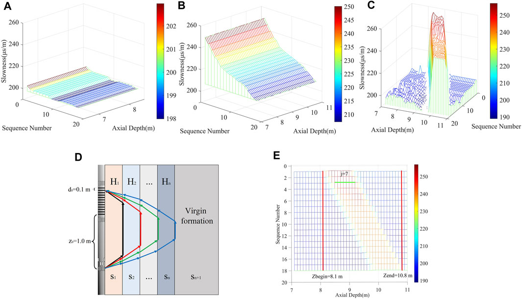
FIGURE 2. Slow sequence characterization. (A) Homogeneous formation slowness sequence; (B) Heterogeneous stratigraphic slowness sequence; (C) Heterogeneous thin beds slowness sequence; (D) Transmission paths of slide wave in radial formation; (E) Quantitative analysis of slow sequences.

2.3 Determine the thin beds

2.3.1 Determine the thickness of the thin beds

In order to conduct the inversion of the radial thickness of the slowness transition zone, the commonly used methods are to update the initial formation model by frequent iteration or obtain an average change profile of slowness in the radial direction at the expense of resolution. The former methods are costly and iteratively time-consuming which are unsuitable for the well-site environment. The latter methods can improve the inversion efficiency but have limited accuracy. In this paper, we propose a scheme based on ray theory to quantitatively determine the layer thickness corresponding to each slowness, to construct the radial profile of slowness distribution in space. The model in Figure 2D shows the transmission paths of slide waves. It is assumed that the transition zone is divided into n layers in radial, and the n+1 $th$ layer is the undisturbed formation. $H_1$ to $H_n$ represent the thickness of different layers in the transition zone, $s_1$ to $s_n$ represent their slowness, and $s_{n+1}$ is the slowness of the undisturbed formation. The number of receivers in the array acoustic logging tool is $N$, receiver internal spacing is $d_0$ and source distance is $z_0$. If we combine every i (i=2,3,4⋯) adjacent receivers in the tool as a group, the average source distance $z_k$ of group k is written as Eq. 6:

${\mathit{z}}_{\mathit{k}}={\mathit{z}}_{\mathbf{0}}+\frac{\left(\mathit{i}+\mathit{k}-\mathbf{2}\right){\mathit{d}}_{\mathbf{0}}}{\mathbf{2}}\mathit{k}=\mathbf{1},\mathbf{2},\cdots ,\left(\mathit{N}-\mathit{i}+\mathbf{1}\right)(6)$

Overall travel time $T_n$ of compressional wave and shear wave travelling within the n $th$ layer is expressed as:

${\mathit{T}}_{\mathit{n}}={\mathit{z}}_{\mathit{k}}{\mathit{s}}_{\mathit{n}+\mathbf{1}}+{\displaystyle \sum _{\mathit{i}=\mathbf{1}}^{\mathit{n}}}\mathbf{2}{\mathit{H}}_{\mathit{i}}\sqrt{{{\mathit{s}}_{\mathit{i}}}^{\mathbf{2}}-{{\mathit{s}}_{\mathit{n}+\mathbf{1}}}^{\mathbf{2}}}(7)$

The time of wave passing through the slowness layer $H_n$ is longer than that of the layer $H_{n-1}$, therefore, the thickness $H_n$ can be obtained according to Eq. 7:

${\mathit{H}}_{\mathit{n}}=\frac{{\displaystyle {\sum }_{\mathit{i}=\mathbf{1}}^{\mathit{n}-\mathbf{1}}}\mathbf{2}{\mathit{H}}_{\mathit{i}}\left(\sqrt{{{\mathit{s}}_{\mathit{i}}}^{\mathbf{2}}-{{\mathit{s}}_{\mathit{n}}}^{\mathbf{2}}}-\sqrt{{{\mathit{s}}_{\mathit{i}}}^{\mathbf{2}}-{{\mathit{s}}_{\mathit{n}+\mathbf{1}}}^{\mathbf{2}}}\right)}{\mathbf{2}\sqrt{{{\mathit{s}}_{\mathit{n}}}^{\mathbf{2}}-{{\mathit{s}}_{\mathit{n}+\mathbf{1}}}^{\mathbf{2}}}}+{\mathit{z}}_{\mathit{k}}\left({\mathit{s}}_{\mathit{n}}-{\mathit{s}}_{\mathit{n}+\mathbf{1}}\right)\mathit{n}=\mathbf{2},\mathbf{3},\cdots (8)$

The thickness $H_1$ of first layer is expressed as:

${\mathit{H}}_{\mathbf{1}}=\frac{{\mathit{z}}_{\mathit{k}}\left({\mathit{s}}_{\mathbf{1}}-{\mathit{s}}_{\mathbf{2}}\right)}{\mathbf{2}\sqrt{{{\mathit{s}}_{\mathbf{1}}}^{\mathbf{2}}-{{\mathit{s}}_{\mathbf{2}}}^{\mathbf{2}}}}(9)$

The depth position corresponding to the slowness sequence can be automatically obtained through Eqs 8, 9. Discrete slowness value points of the surrounding wellbore can be obtained by repeating this step at every sampling depth. In the subsequent inversion of this paper, we combine 21 receivers in groups of 4 to obtain a slowness sequence with 18 slowness values.

2.3.2 Determine the axial position of the thin beds

After we obtain the radial slowness distribution of thin beds, we need to determine the axial position of the thin beds to complete its characterization. The axial thickness of thin beds is obtained based on a simple assumption, as shown in the model of Figure 1A. When the thin bed happens to be located just above the last receiver, the radial heterogeneity of the thin bed changes the slowness sequence when the instrument is lifted. This change causes the slowness sequence to increase first, then stay the same, and finally decrease. The number of sequences with the enormous change reflects the thickness of the thin bed which is related to the single lift of the instrument $L$. Based on this consideration, we need to eliminate the influence of the number of our receiver combinations and the receiver spacing. The axial thickness $H_a$ can be expressed as:

${\mathit{H}}_{\mathit{a}}=\mathit{j}\mathit{L}+\frac{{\mathit{i}\mathit{d}}_{\mathbf{0}}}{\mathbf{2}}(10)$

Where $j$ represents the number of slowness sequences with significant variation. As shown by the green line in Figure 2E, the number of slowness sequences with significant variation are 7. The same applies to the axial position of the thin bed, when the thin bed is just above the last receiver, the depth recording point is larger than half the length of the receiver array. When the instrument mentions that the thin bed is located below our first receiver, the depth recording point is less than half the length of the receiver array. In this way, the axial position of the thin bed is related to the axial depth where the slowness change occurs. The axial centre position of the thin bed $Z_c$ can be expressed as Eq. 11:

${\mathit{Z}}_{\mathit{c}}=\frac{{\mathit{Z}}_{\mathit{b}\mathit{e}\mathit{g}\mathit{i}\mathit{n}}+{\mathit{Z}}_{\mathit{e}\mathit{n}\mathit{d}}}{\mathbf{2}}(11)$

Where $Z_{begin}$ and $Z_{end}$ represent the starting and ending positions where the slowness sequences variation. As shown by the red line in Figure 2E, the starting position of slowness sequences variation $Z_{begin}$ is 8.1 m, the ending position of slowness sequences variation $Z_{end}$ is 10.8 m. The axial centre position of the thin bed $Z_c$ is 9.45 m which restored the position of thin beds in the formation model.

2.4 Slowness interpolation imaging

When we get the radial slowness distribution, it means that we get a two-dimensional profile of radial distance and slowness value. In order to make it easier to observe, we use the IDW interpolation method (Lu and Wong, 2008) on the two-dimensional profile to make it an image. The IDW method is a commonly used deterministic model for spatial interpolation, popular among geoscientists due to its calculation speed and interpretability. It assumes that the attribute value of an unsampled point is the weighted average of known values within the neighbourhood, and the weights are inversely related to the distances between the prediction location and the sampled locations. The IDW method is modified by a constant power or a distance-decay parameter to adjust the diminishing strength in a relationship with increasing distance. The IDW formulas are given as Eqs 12, 13:

${\widehat{\mathit{s}}}_{\mathit{p}}={\displaystyle \sum _{\mathit{i}}^{\mathit{n}}}{\mathit{w}}_{\mathit{i}}{\mathit{s}}_{\mathit{i}}(12)$

${\mathit{w}}_{\mathit{i}}=\frac{{{\mathit{d}}_{\mathit{i}}}^{-\mathit{\alpha }}}{{\displaystyle {\sum }_{\mathit{i}=\mathbf{1}}^{\mathit{n}}}{{\mathit{d}}_{\mathit{i}}}^{-\mathit{\alpha }}}(13)$

where ${\widehat{s}}_p$ means the unknown slowness data; $s_i$ means the known slowness data though Eq. 3; $n$ means the amount of slowness sequence; $w_i$ means the weighting of each slowness sequence; $d_i$ means the distance from each discrete slowness value to the unknown site; $\alpha$ means the power, and is also a control parameter, generally assumed as 2 (Zhu and Jia, 2004). We can use interpolation to obtain the spatial dispersion slowness of the thin bed and ultimately image its slowness.

3 Results

3.1 Synthetic example

In this section, we study the effects of the changes in axial thickness, axial position, and invasion degree of thin bed on the slowness sequences, and the results show that the slowness sequences are sensitive to the above three conditions and manifest themselves as a single variable characteristic manifests. For convenience, the initial position of the sound source and the instrument is the same as in Section 2.1, and the axial centre position of the thin bed is at 9.5 m. The default intrusion of the thin bed is that the longitudinal compressional wave changes from 4000m/s-4800 m/s in five steps, the step change is 200 m/s, the radial distance of each step is 0.15 m, the total intrusive radial distance is 0.75 m. The original formation compressional wave velocity is 5000 m/s, as shown in Figure 1D. We simulated the axial thickness of the thin bed at 1.0 m, 0.8 m, 0.6 m, and 0.4 m, respectively. Figures 3A–D represent the slowness sequence results corresponding to the instrument lifting by 4.0 m. The results show that only changing the thin bed’s axial thickness affects the number of slowness sequences with significant variation $j$ and does not change the starting and ending positions of slowness sequences variation $Z_{begin}$ and $Z_{end}$. Figure 3E represents the slowness sequence result when the instrument is raised by 4.0 m without changing the thin bed’s axial position and thickness. The new intrusion case is that the compressional wave changes in five steps from 4500 m/s to 4900 m/s, and the amount of change in each step is 100 m/s. The results indicate that only changing the intrusion situation affects the range of slowness variation without changing the number of slowness sequences with significant variation $j$ and the starting and ending positions of slowness sequences variation $Z_{begin}$ and $Z_{end}$. Figures 3F, G represent the addition of thin beds with a centre position of 8.5 m and 7.5 m without changing the thin bed properties, and the instrument lifting by 6.0 m and 7.0 m. The results show that changing the thin bed’s axial position affects the starting and ending positions of slowness sequences variation $Z_{begin}$ and $Z_{end}$ and does not change the number of slowness sequences with significant variation $j$ and the range of slowness variation.

FIGURE 3

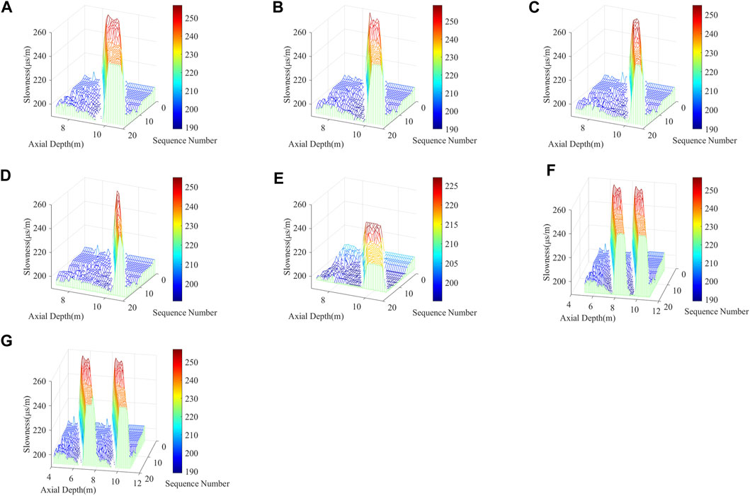
FIGURE 3. Slow sequence cases under different conditions. (A) Thin bed axial thickness of 1.0 m; (B) Thin bed axial thickness of 0.8 m; (C) Thin bed axial thickness of 0.6 m; (D) Thin bed axial thickness of 0.4 m; (E) Slowness change in the invasive zone is reduced; (F) Two thin beds with axial thickness of 1.0 m spaced 1.0 m; (G) Two thin beds with axial thickness of 1.0 m spaced 2.0 m.

Obtaining the $j$ values of Figures 3A–D respectively, we can obtain that $j$ is 8, 6, 4 and 2, and bring into Eq. 10 to calculate $H_a$ of 1.0 m, 0.8 m, 0.6 m and 0.4 m, which are consistent with the formation model. From Figure 3E, it can be seen that the slowness change area is similar to the formation model. Acquire $Z_{begin}$ and $Z_{end}$ in Figure 3F, $Z_{begin1}$ is 6.1 m and $Z_{end1}$ is 8.8 m, $Z_{begin2}$ is 8.1 m and $Z_{end2}$ is 10.8 m, $Z_{c1}$ and $Z_{c2}$ are calculated to be 9.45 m and 7.45 m. Similarly, $Z_{c3}$ and $Z_{c4}$ in Figure 3G are 9.45 m and 6.45 m, which restored the position of thin beds in the formation model. Then, we verify whether the heterogeneous formation’s correct slowness distribution can be restored. We first establish a formation with total well intrusion, with a maximum intrusion depth of 0.4 m and a velocity varying every 0.05 m, from 4,000 m/s to 5,000 m/s. The formation model is shown in Figure 4A. The proposed method is used to invert its radial compression wave slowness (results are expressed in compression wave velocity). The inversion result is highly consistent with the formation model, as shown in Figure 4B. Next, we consider the presence of both thin beds and radial intrusion. We build a total of 16 m deep formation model. At 3.5 m–4.5 m, we set up a thin bed with a thickness of 1.0 m. The radial invasion depth of this thin bed is 0.8 m, with velocity changing every 0.2 m, and the velocities are 4,000 m/s, 4,200 m/s, 4,400 m/s, and 4,600 m/s, respectively. At 13.75 m–14.25 m, we set up another thin bed with a thickness of 0.5 m. The radial invasion depth of this thin bed is 0.4 m, with velocity changing every 0.1 m, and the velocities are 4,000 m/s, 4,100 m/s, 4,200 m/s, and 4,300 m/s, respectively. The formation model is shown in Figure 4C. In the inversion results, we find that the radial slowness variation and the position of the axial thin layer were accurately described, which is highly consistent with the stratigraphic model, which is shown in Figure 4D. Synthetic data verified the effectiveness and accuracy of the proposed method.

FIGURE 4

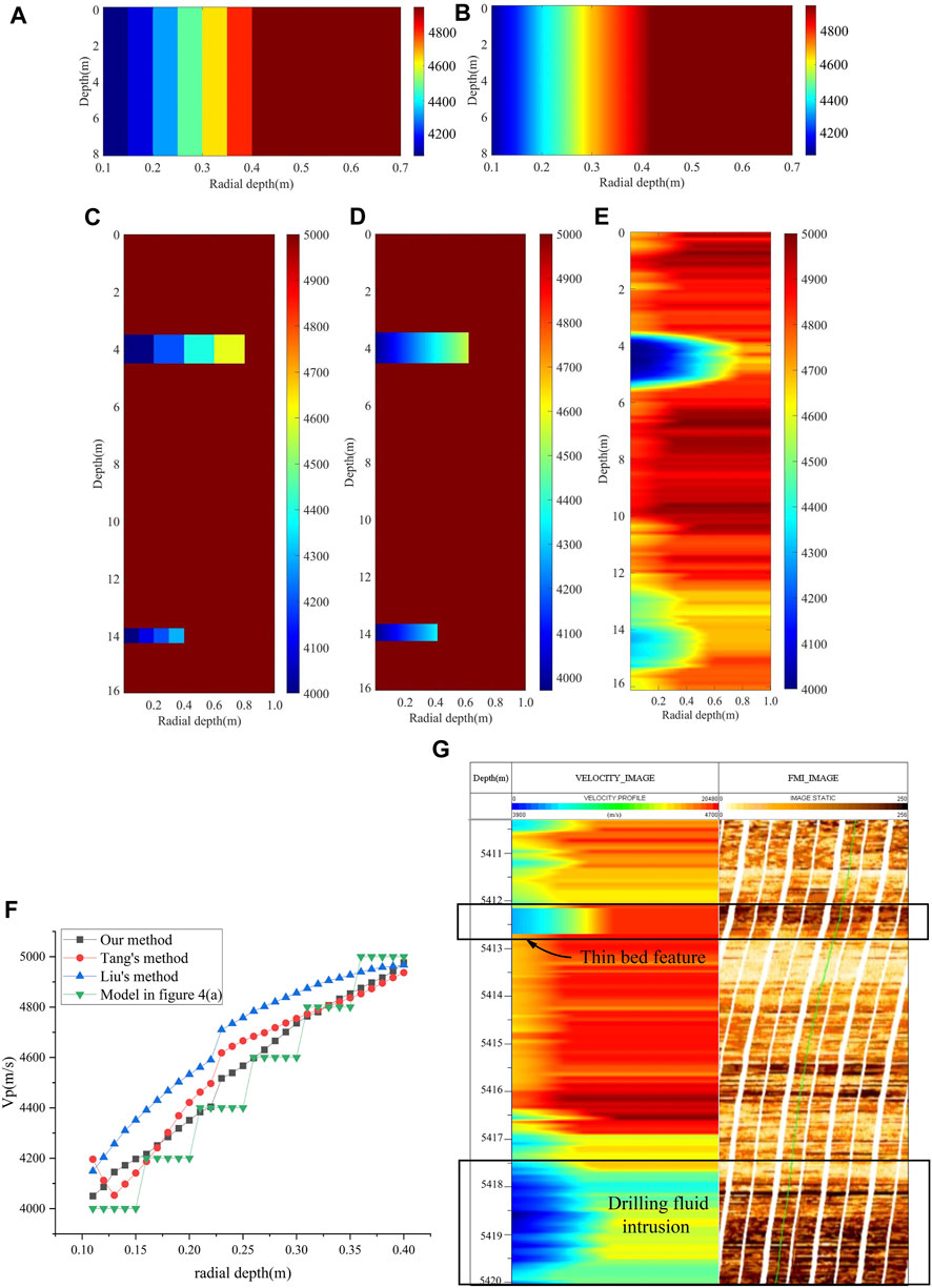
FIGURE 4. Thin beds slowness imaging inversion result. (A) Formation model with radial velocity variation only; (B) Inversion result of radial velocity variation only; (C) Formation model with different axial thicknesses and radial intrusion thin beds; (D) Inversion results of the proposed method; (E) Axial resolution limitations of conventional methods; (F) Radial slowness accuracy with different methods. (G) Inversion result of field data (black wireframes indicate thin bed and drilling fluid intrusion).

3.2 Applicability analysis

In this section, we will compare the radial accuracy and axial resolution of the new method with other methods to illustrate the superiority of the new method. We first use the conventional method to deal with the formation model containing the thin bed (Figure 4C). By observing the inversion result in Figure 4E, we can find the inversion results can qualitatively observe the position of formation velocity change. However, the conventional method cannot describe the specific thickness of the thin bed. This is because the theory of conventional methods assumes that the receiving array area is a homogeneous formation. When thin beds are encountered since conventional methods average the contribution of the thin beds over the entire length of the receiving array, the axial range of the velocity variation is much larger than the thickness of the thin beds, and the radial velocity distribution is closer to the near-wellbore formation velocity. In contrast, the proposed method dramatically improves the axial resolution of velocity inversion, making it able to distinguish thin layers with a minimum thickness of 0.5 m and realize the nuanced characterization of the reservoir. Next, the radial accuracy of the proposed method is compared with other methods. We use both Tang’s and Liu’s radial slowness inversion method to treat the radial intrusion formation in Figure 4A and then compare the inversion results from our proposed method with them. Through the observation of Figure 4F, it is found that both the proposed method and the two methods can reflect the changes of invasion to a certain extent. Tang’s method is to constrain the high-frequency signal in the frequency domain, which causes errors in the near-hole region, and the radial velocity can be observed to decrease first and then increase in the inversion results. Although the results obtained by Liu’s method are accurate in near-hole and far-hole positions, but the overall inversion velocity is slightly higher than the actual value. The inversion results of our proposed method in near and far boreholes are similar to those of Tang and Liu’s method, and the overall inversion accuracy is higher than those of the two methods. This shows that the proposed method can increase the axial resolution while ensuring the accuracy of radial inversion.

3.3 Field example

We apply this new method to field data processing in western China. With the field data of Well X1, the constructed radial velocity and FMI static results from 5,410 m to 5,420 m are shown in Figure 4G. Lateral resistivity logging results from 5,410 m to 5412.2 m and 5,416.3 m–5420.0 m indicate varying degrees of invasion in these two depth intervals, and the invasion degree is stronger from 5,416.3 m to 5,420.0 m. It can be seen from the results that the near-wellbore velocity from 5,410 m to 5412.2 m has slightly decreased, which can be interpreted as weak intrusive heterogeneous formations. Similarly, the near-wellbore velocity from 5,416.3 m to 5420.0 m has significantly decreased, which can be interpreted as strong intrusive heterogeneous formations. The above two results have good consistency with the lateral logging results.

The FMI static results show two evident dark bands from 5,412.2 m to 5412.6 m and 5,418.2 m–5420.0 m. This is due to the intrusion of near-well drilling fluid into the formation, which makes the resistivity of the invaded formation less than that of the uninvaded formation. This also reflects the presence of thin bed intrusion from 5,412.2 m to 5412.6 m and drilling fluid intrusion at 5,416.3 m–5420.0 m. The velocity inversion results are in good agreement with the FMI static results, which reflects the accuracy and reliability of the inversion method.

4 Conclusion

We propose a new method to perform the thin bed’s slowness imaging. The method can automatically extract the radial slowness sequences from the array acoustic logging data and identify the formation conditions corresponding to different slowness sequences. By extracting the required parameters from the slowness sequence and incorporating them into the quantitative solution formula, the axial thickness, axial centre position, radial slowness, and radial thickness of the thin bed can be obtained. This method can effectively improve the axial resolution in logging and responds well to thin bed identification. The synthesized examples and field examples jointly demonstrate the stability and reliability of the thin bed slowness imaging method.

Data availability statement

The original contributions presented in the study are included in the article/Supplementary material, further inquiries can be directed to the corresponding author.

Author contributions

ZW: Conceptualization, Formal Analysis, Methodology, Software, Writing–original draft. WY: Funding acquisition, Project administration, Supervision, Validation, Writing–review and editing.

Funding

The author(s) declare financial support was received for the research, authorship, and/or publication of this article. This research was funded by National Natural Science Foundation of China, grant number 42174129 and 41374143.

Conflict of interest

The authors declare that the research was conducted in the absence of any commercial or financial relationships that could be construed as a potential conflict of interest.

Publisher’s note

All claims expressed in this article are solely those of the authors and do not necessarily represent those of their affiliated organizations, or those of the publisher, the editors and the reviewers. Any product that may be evaluated in this article, or claim that may be made by its manufacturer, is not guaranteed or endorsed by the publisher.

References

Backus, G., and Gilbert, F. (1970). Uniqueness in the inversion of inaccurate gross Earth data. Math. Phys. Sci. 266. 1173. 123-192. doi:10.1098/rsta.1970.0005

CrossRef Full Text | Google Scholar

Baker, L. J., and Winbow, G. A. (1988). Multipole P-wave logging in formations altered by drilling. Geophysics 53, 1207–1218. doi:10.1190/1.1442561

CrossRef Full Text | Google Scholar

Cheng, N., Cheng, C. H., and Toksöz, M. N. (1995). Borehole wave propagation in three dimensions. J. Acoust. Soc. Am. 97 (6), 3483–3493. doi:10.1121/1.412996

CrossRef Full Text | Google Scholar

Dines, K. A., and Lytle, R. J. (1979). Computerized geophysical tomography. Proc. IEEE 67 (7), 1065–1073. doi:10.1109/PROC.1979.11390

CrossRef Full Text | Google Scholar

Hornby, B. E. (1993). Tomographic reconstruction of near-borehole slowness using refracted borehole sonic arrivals. Geophysics 58 (12), 1726–1738. doi:10.1190/1.1443387

CrossRef Full Text | Google Scholar

Huang, S., and Torres-Verdin, C. (2016). Inversion-based interpretation of borehole sonic measurements using semianalytical spatial sensitivity functions. Geophysics 81 (2), D111–D124. doi:10.1190/geo2015-0335.1

CrossRef Full Text | Google Scholar

Kimball, C. V., and Marzetta, T. L. (1984). Semblance processing of borehole acoustic array data. Geophysics 49 (3), 274–281. doi:10.1190/1.1441659

CrossRef Full Text | Google Scholar

Lei, T., Zeroug, S., Bose, S., Prioul, R., and Donald, A. (2019). Inversion of high-resolution high-quality sonic compressional and shear logs for unconventional reservoirs. Petrophysics - SPWLA J. Form. Eval. Reserv. Descr. 60 (06), 697–711. doi:10.30632/T60ALS-2019_QQQ

CrossRef Full Text | Google Scholar

Liu, Y., Chen, H., Li, C., He, X., Chai, D., Habibi, D., et al. (2021). Radial profiling of near-borehole formation velocities by a stepwise inversion of acoustic well logging data. J. Petroleum Sci. Eng. 196, 107648. doi:10.1016/j.petrol.2020.107648

CrossRef Full Text | Google Scholar

Lu, G. Y., and Wong, D. W. (2008). An adaptive inverse-distance weighting spatial interpolation technique. Comput. Geosciences 34 (9), 1044–1055. doi:10.1016/j.cageo.2007.07.010

CrossRef Full Text | Google Scholar

Ma, M., Chen, H., He, X., and Wang, X. (2013). The inversion of shear wave slowness's radial variations based on the dipole flexural mode dispersion. Chin. J. Geophys 56 (6), 2077–2087. doi:10.6038/cig2013062

CrossRef Full Text | Google Scholar

Pistre, V., Kinoshita, T., Endo, T., Schilling, K., and Pabon, J. (2005). “A modular wireline sonic tool for measurements of 3D (azimuthal, radial, and axial formation acoustic properties),” in SPWLA 46th Annual Logging Symposium, New Orleans, LA, USA, June 2005. SPWLA-2005-P.

Google Scholar

Sayers, C. M., Adachi, J., and Taleghani, A. D. (2008). “The effect of near-wellbore yield on elastic wave velocities in sandstones,” in SEG technical program expanded abstracts 2008: society of exploration geophysicists, Society of Exploration Geophysicists, Houston, TX, USA, 339–343. doi:10.1190/1.3054818

CrossRef Full Text | Google Scholar

Sinha, B. K., Vissapragada, B., Kisra, S., Sunaga, S., Yamamoto, H., Endo, T., et al. (2005). “Optimal well completions using radial profiling of formation shear slownesses,” in Spe Technical Conference and Exhibition, Dallas, TX, USA, October 2005. doi:10.2118/95837-MS

CrossRef Full Text | Google Scholar

Sinha, B. K., Vissapragada, B., Renlie, L., and Tysse, S. (2006). Radial profiling of the three formation shear moduli and its application to well completions. Geophysics 71, E65–E77. doi:10.1190/1.2335879

CrossRef Full Text | Google Scholar

Tang, X., and Patterson, D. J. (2010). Mapping formation radial shear-wave velocity variation by a constrained inversion of borehole flexural-wave dispersion data. Geophysics 75 (6), E183–E190. doi:10.1190/1.3502664

CrossRef Full Text | Google Scholar

Tang, X., Xu, S., Zhuang, C., Su, Y., and Chen, X. (2016). Quantitative evaluation of rock brittleness and fracability based on elastic-wave velocity variation around borehole. Petroleum Explor. Dev. 43 (3), 457–464. doi:10.1016/S1876-3804(16)30053-2

CrossRef Full Text | Google Scholar

Winkler, K. W. (2005). Borehole damage indicator from stress-induced velocity variations. Geophysics 70 (1), F11–F16. doi:10.1190/1.1852772

CrossRef Full Text | Google Scholar

Xu, S., and White, R. E. (1995). A new velocity model for clay-sand mixtures1. Geophys. Prospect. 43 (1), 91–118. doi:10.1111/j.1365-2478.1995.tb00126.x

CrossRef Full Text | Google Scholar

Zeroug, S., Valero, H., Bose, S., and Yamamoto, H. (2006). “Monopole radial profiling of compressional slowness,” in SEG technical program expanded abstracts 2006: society of exploration geophysicists, Society of Exploration Geophysicists, Houston, TX, USA, 354–358. doi:10.1190/1.2370275

CrossRef Full Text | Google Scholar

Zhu, H. Y., and Jia, S. (2004). Uncertainty in the spatial interpolation of rainfall data. Prog. Geogr. 23 (2), 34–42. doi:10.11820/dlxjz.2004.02.005

CrossRef Full Text | Google Scholar