 Xin Guo
 Jianhu Gao
- Research Institute of Petroleum Exploration and Development-Northwest (NWGI), Lanzhou, China
During the propagation of seismic waves underground, the high-frequency seismic response of thin reservoir is absorbed and attenuated, which poses a challenge in seismic thin reservoir prediction. The high-resolution processing techniques have the capability to significantly expand the frequency range of the seismic data, so it becomes a key technique for thin reservoir prediction. Most of these techniques necessitate the extraction of seismic wavelets. However, the spatial and temporal variations of seismic data result in multiple solutions for wavelet extraction. Simultaneously, the majority of techniques fail to consider the influence of spatial tectonic features on the high-resolution processing. In this paper, we propose a novel solution to address these two fundamental challenges by utilizing seismic spectral expansion, sparse reflection coefficients, and spatial continuity constraints. First, we propose an innovative spectral fitting method that aims to expand the frequency bandwidth while adhering to the desired wavelet constraints. This method allows us to fully utilize the effective frequency information. It not only obtains broadband seismic data but also captures precise wavelets. Then, sparse deconvolution is employed to further extend the frequency range by utilizing the accurately expected wavelet and obtaining a high-resolution reflection coefficient. Finally, the Hessian matrix regularization is employed to constrain the spatial continuity of the reflection coefficient. This method is validated in both the model and real seismic data. Compared to traditional sparse deconvolution and spectral modeling deconvolution with spatial constraints, this method not only expands the frequency bandwidth and enhances seismic resolution but also preserves operational frequency information and improves the spatial continuity of seismic data. It has been verified that this approach can be used to forecast thin reservoir and reconstruct spatial tectonic characteristics.
1 Introduction
In the field of petroleum seismic exploration, it is essential to have high-quality seismic data to carry out tasks like detecting weak seismic signals, forecasting thin reservoirs, identifying minor faults, and precisely dividing sequences. Domestic and foreign scholars have conducted numerous studies on seismic high-resolution processing, including deconvolution, spectral whitening, inverse Q filtering, sparse optimization, wavelet decomposition, deep learning, and other technologies. These technologies and methods have significantly contributed to the development of seismic high-resolution processing. However, they also have their advantages and disadvantages.
The principle of deconvolution involves the compression of the seismic wavelet in order to improve the resolution of seismic data. The integration of sparse constraints into the deconvolution process was initially introduced, resulting in a notably efficient technique. (Taylor et al., 1979). Many scholars have focused on optimizing this theory, and their research is divided into two main aspects: the accurate acquisition of seismic wavelets and the application of various constraints. Extracting accurate seismic wavelet is critical (Baziw and Ulrych, 2006; Mirko and pham, 2008; Sacchi, 2010; Nasser and Mauricio, 2014; Macedo et al., 2016; Cabrera et al., 2020). These researchers analyzed and optimized seismic wavelets and proposed various methods for sparse deconvolution. Numerous scholars have studied optimization methods for seismic inverse problems, including sparse constraints, impedance constraints, and algorithm optimization (Velis, 2008; Gholami and Sacchi, 2012; Chen and Zong, 2022). These methods have been investigated for addressing geophysical inverse problems. Different constraints are integrated into the procedure of addressing the inverse problem to improve the precision of seismic forecasting outcomes. Meanwhile, it can be noted that there is consistency between seismic data and the principles of underground geology. Throughout the process of deposition, sediments display stratified characteristics, and the seismic data indicate the fluctuations in the stratums of rock. This should also be evident as a continuous trait. Many scholars have conducted extensive research in this area (Heimer and Cohen, 2009; Gholami and Sacchi, 2012; Gholami and Sacchi, 2013; Li et al., 2013; Yuan et al., 2016; Du et al., 2018; Ma et al., 2020). The focus of these studies has mainly been on the spatial continuity of seismic data. These studies have led to the development of high-resolution seismic data processing. Nevertheless, the constraints associated with these approaches, particularly the challenges in accurately estimating wavelets, result in inconsistent outcomes when applied.
Compressing seismic wavelets and enhancing seismic resolution can be accomplished by employing frequency domain computations, particularly through the utilization of spectral modeling techniques. It improves the resolution of seismic data by fitting the spectrum of seismic records, extracting a smooth wavelet amplitude spectrum and expanding it to increase the frequency range. The spectral modeling method also suffers from the challenge of accurately obtaining the spectrum of the seismic wavelet. The construction of the wavelet spectrum is primarily accomplished by smoothly fitting seismic data (Rosa and Ulrych, 1991). Some scholars have also noticed that the wavelet spectrum is, in fact, the low-frequency component of the amplitude spectrum of seismic records. As a result, the concept of the quadratic spectrum was proposed (Tang et al., 2010). Other scholars have also discovered that seismic wavelets are time-varying, which leads to a modification of seismic spectral characteristics. They have proposed a method for constructing a time-varying wavelet spectrum (Guo et al., 2015; Wang et al., 2017; Yuan et al., 2017). In the construction of the spectral modeling method, challenges arise not only in relation to the wavelet spectrum but also in regard to the three-dimensional spatial configuration. Therefore, a spectral modeling method based on the constraint of spatial continuity is proposed (Guo et al., 2022). These methods have been studied from the perspectives of frequency domain wavelet extraction, time-frequency characteristic patterns, and constraint optimization algorithms and have yielded improved results.
The method presented in this paper is based on the concept of seismic spectrum modeling deconvolution. This method assumes that the seismic wavelet is zero-phase. Firstly, the process of broadening the spectrum is achieved through the application of the seismic frequency division fusion technique, with limitations imposed by the desired wavelet. It not only expands the bandwidth but also provides an accurate estimation of the wavelet spectrum of seismic data. Secondly, the objective function in the time domain is augmented with the L1 regularization sparse constraint, which is based on the seismic record and the expected seismic wavelet. This augmentation allows for the estimation of the seismic reflection coefficient. Finally, the Hessian matrix regularization constraint is employed to control the spatial coherence of the seismic reflection coefficient, taking into account the spatial coherence of geological strata. The proposed method does not require the extraction of seismic wavelets. The simultaneous implementation of spectrum expansion and sparse optimization leads to enhanced resolution and preservation of high fidelity in seismic data. The high-resolution seismic data processed by this method have higher confidence for subsequent seismic interpretation and reservoir prediction.
2 Theories and methods
2.1 Spectrum expansion
According to the seismic convolution model, the seismic signal is generated by the convolution of the seismic reflection coefficient with the seismic wavelet in the time domain. In the frequency domain, the seismic signal spectrum is calculated by multiplying the amplitude spectrum and the phase spectrum of the seismic signal as follows:
where the left side of the equivalent is defined as Eqs 1-1, and
According to Eq. 1, the deconvolution procedure entails the compression of the seismic wavelet, leading to an expansion of the seismic frequency band in the frequency domain. Therefore, determining the range of frequency broadening is very important. The technique of seismic record spectrum scanning can help determine the effective frequency bandwidth. The limited band information is 4–64 Hz, as shown in Figure 1. In practical applications, it is advisable to use a narrower scanning interval band. Then, the distribution of effective information within the band can be more accurately determined.
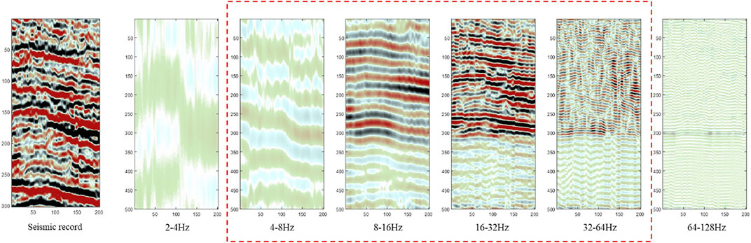
FIGURE 1. Practical seismic record and different frequency division scanning sections.
According to the results of the spectrum scanning, the spectrum fitting method is employed to expand the frequency range within the effective frequency band. Then, the octave can be increased to enhance seismic resolution. In this paper, the spectral fitting method adopts a frequency division weighted superposition approach. At first, Gaussian functions are constructed in different frequency bands. These functions are subsequently employed for frequency division processing, as depicted in Figure 2A. The Gaussian functions of different frequency bands are expressed as
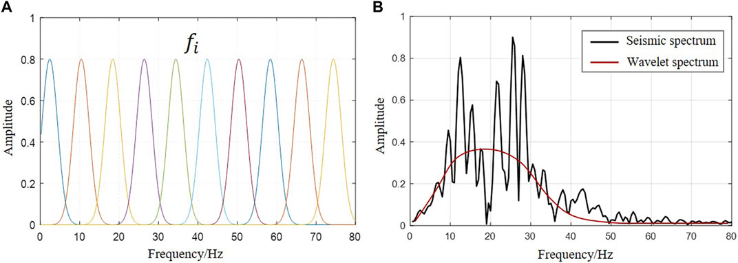
FIGURE 2. (A) Gaussian frequency division curve and (B) Amplitude spectrum and wavelet spectrum of the seismic record.
Gaussian functions with different frequencies are employed to limit the amplitude spectrum of the seismic record, leading to the acquisition of seismic frequency division amplitude spectra (illustrated by the colored line in Figure 3A). According to the results of spectrum scanning, the desired range of wavelet amplitude spectrum can be determined accordingly. The amplitude spectra of the frequency division are weighted and superimposed, and the expansion of the spectrum is performed while adhering to the constraints of the desired wavelet amplitude spectrum, as below:
where
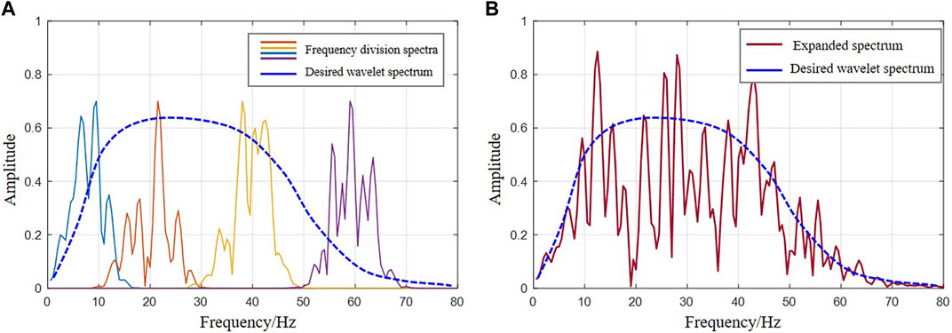
FIGURE 3. (A) Gaussian frequency division spectra and (B) Wide spectrum constrained by expected wavelet spectrum.
2.2 Sparse optimization
Following the acquisition of high-resolution seismic data and wavelets through the spectral fitting method, it is possible to conduct sparse deconvolution. The conventional method for sparse deconvolution involves constructing a sparse objective function when the wavelet is known. This can be done as follows:
where
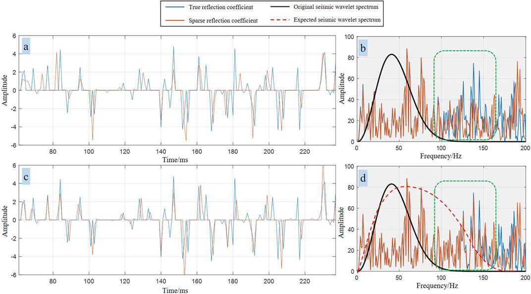
FIGURE 4. Comparison of the effects of traditional sparse deconvolution and the sparse deconvolution method proposed in this paper. (A) The reflection coefficient by traditional spare deconvolution; (B) The spectra of the true reflection coefficient (blue line) and sparse deconvolution reflection coefficient (red line); (C) The reflection coefficient by the proposed method; (D) The spectra of the true reflection coefficient (blue line) and the reflection coefficient by the proposed method (red line).
In order to achieve a precise sparse reflection coefficient, it is essential to capture accurate spectral properties of high-frequency signals. According to Eq. 2 and Eq. 1, it is easy to establish a relationship between the seismic spectrum and the seismic reflection coefficient.
Where
Where
After obtaining the weight coefficient
The recently developed objective function offers two benefits in comparison to conventional sparse deconvolution techniques. The initial point to consider is the elimination of the necessity to extract the wavelet, thereby mitigating potential errors in the extraction of the seismic wavelet. The second point is that the expected wavelet encompasses a wider spectrum of frequencies, resulting in a more accurate restoration of spectral characteristics. Compared with Figures 4A,C, the two sparse deconvolution methods show significant differences in the reflection coefficient. Figure 4C depicts the outcome of the application of the proposed method, demonstrating a significantly improved accuracy in the estimation of the inverted reflection coefficient. The primary factor is that the conventional sparse deconvolution method cannot effectively handle the spectral characteristics of high-frequency seismic records (green curve in Figure 4B). This results in a notable disparity between the calculated reflection coefficient and the true value. The sparse deconvolution method proposed in this paper is closer to the true seismic reflection coefficient because it can more effectively restore the spectral characteristics of high-frequency seismic signals (as depicted by the green curve in Figure 4D). This demonstrates the effectiveness of the objective function in this paper.
2.3 Spatial continuity constraints
There are differences in the reflection coefficients obtained by the sparse deconvolution method in different seismic channels, encompassing discrepancies in time bias and amplitude fluctuations. These differences contradict the expected gradual lateral transition of geological features. So, the spatial continuity constraints are essential for achieving sparse solving while maintaining constructive control.
The first-order differential matrix, commonly referred to as total variation (TV) regularization, lead to a step-like effect that is not appropriate for spatial control constraints. The second-order differential matrix possesses smooth characteristics, enabling it to preserve the surface of three-dimensional data and ensure the spatial continuity of seismic data. In this paper, the method of regularizing the Hessian matrix is used to impose spatial continuity constraints. The Hessian matrix is composed of multiple second-order differential matrices. Assuming the three-dimensional seismic data is
where
The regularization of the Hessian matrix can be expressed as:
where
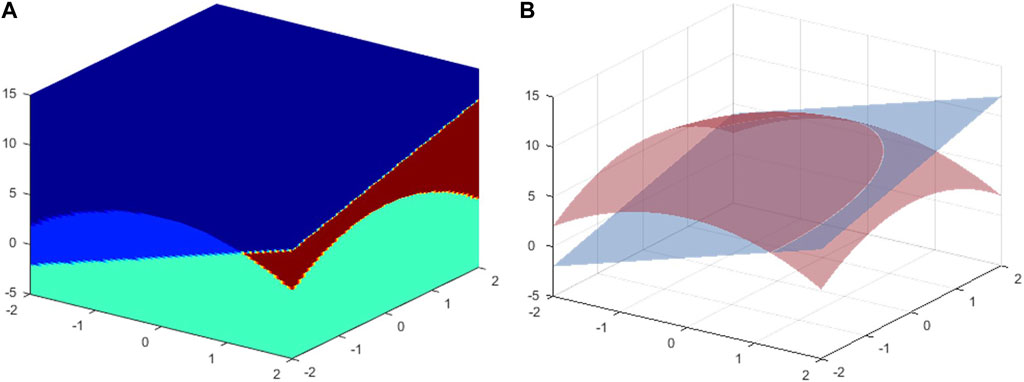
FIGURE 5. (A) 3D geological model with two stratigraphic interfaces and (B) The Hessian Frobenius norm shows the smooth interface.
In order to be able to optimize the solution for seismic data
where
Combine Eqs 6, 9 to get the final objective function:
where
Where,
3 Model validation
To confirm the advantages of the method proposed in this paper, a geological model is constructed (Figure 6A). The geological model includes three sets of thin reservoirs with a thickness range of 0–15 m. These reservoirs are utilized for evaluating the effectiveness of various methods in thin reservoir prediction, as depicted in Figure 6A (①②③). The synthetic seismic record was generated by convolving a seismic wavelet with a reflection coefficient obtained from the geological model (Figure 6B). The seismic wavelet is a Ricker wavelet with a main frequency of 25 Hz. Gaussian noise (S/N=3) was added to the synthetic seismic record to simulate the noisy seismic record (Figure 6C). The S/N is the ratio of the amplitude of the true seismic signal to that of the noise.
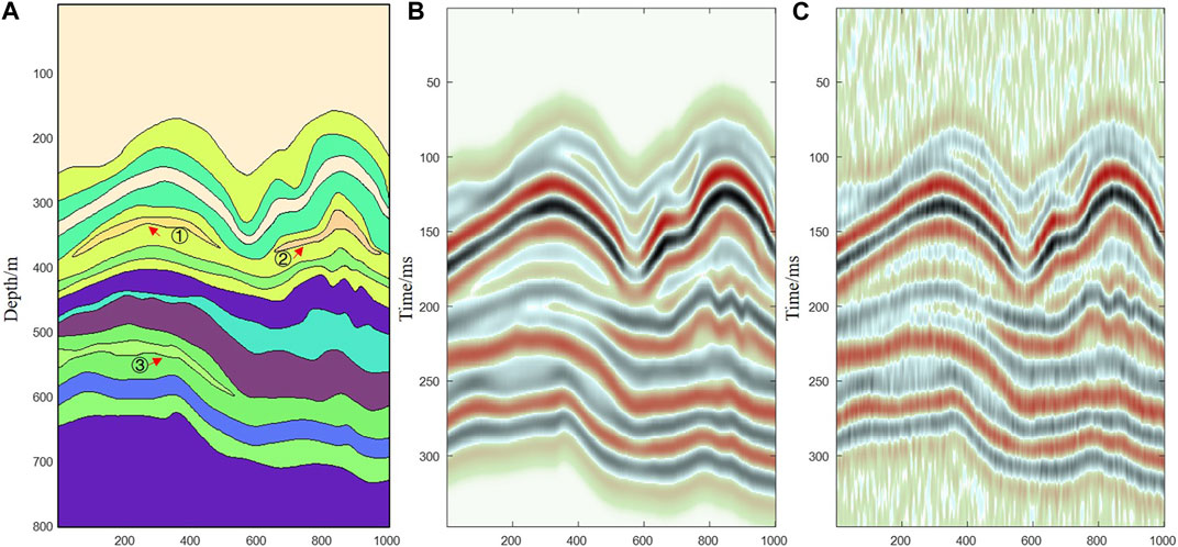
FIGURE 6. (A) Geological model with three sets of thin reservoir shown as ①②③; (B) Synthetic seismic record convolved with Ricker wavelet of main frequency 25Hz; (C) Synthetic seismic record with Gaussian noise of S/N=3.
Different methods are employed for the analysis of the seismic data containing noise as depicted in Figure 6C. Since the proposed method can obtain both the seismic reflection coefficient and high-resolution seismic records, this paper compares it with various conventional methods. Firstly, Figure 7 shows the application effect of the proposed method and the sparse deconvolution method. Figure 7A represents the actual seismic reflection coefficient. Figure 7B illustrates the seismic reflection coefficient that has been computed through the utilization of sparse deconvolution. Figure 7C shows the seismic reflection coefficient computed utilizing the method in this paper. The method presented in this paper is more accurate for recovering the reflection coefficient. The main reason is that the proposed method incorporates a spatial continuity constraint, resulting in improved interface continuity of the solved seismic reflection coefficient compared to the conventional sparse deconvolution method. Meanwhile, the spectral fitting method is more accurate in recovering seismic spectrum features. The inversion of high-frequency information in seismic signals provides more accurate and detailed information. It also improves the precision of thin reservoir responses, as indicated by the arrow in the figure. Additionally, it improves the high-resolution fidelity of seismic data.
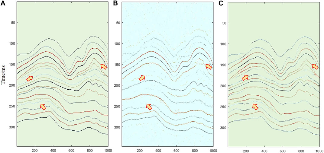
FIGURE 7. (A) True seismic reflection coefficient; (B) The solved reflection coefficient by sparse deconvolution; (C) The solved reflection coefficient by the proposed method.
In practical use, obtaining seismic data with high resolution is essential for subsequent attribute analysis and seismic inversion. Figure 8A shows a seismic record containing Gaussian noise. Figure 8B is a high-resolution seismic section processed using spectral modeling deconvolution with spatial continuity constraints. Figure 8C is a high-resolution seismic section processed using the proposed method. The process of spectral fitting exists in both methods, so the overall spectral range is basically the same, and the range has been extended from the initial 5–45 Hz to approximately 5–65 Hz. The difference between Figures 8B,C is the variation in spatial continuity. The spatial continuity refers to the characteristics of the seismic waveform in Figure 8B and the seismic reflection coefficient in Figure 8C. It can be seen that the high-resolution seismic results, constrained by the seismic reflection coefficient (Figure 8C), demonstrate superior noise cancellation compared to those depicted in Figure 8B. Meanwhile, the proposed method provides more accurate spatial constraints for thin reservoir information.
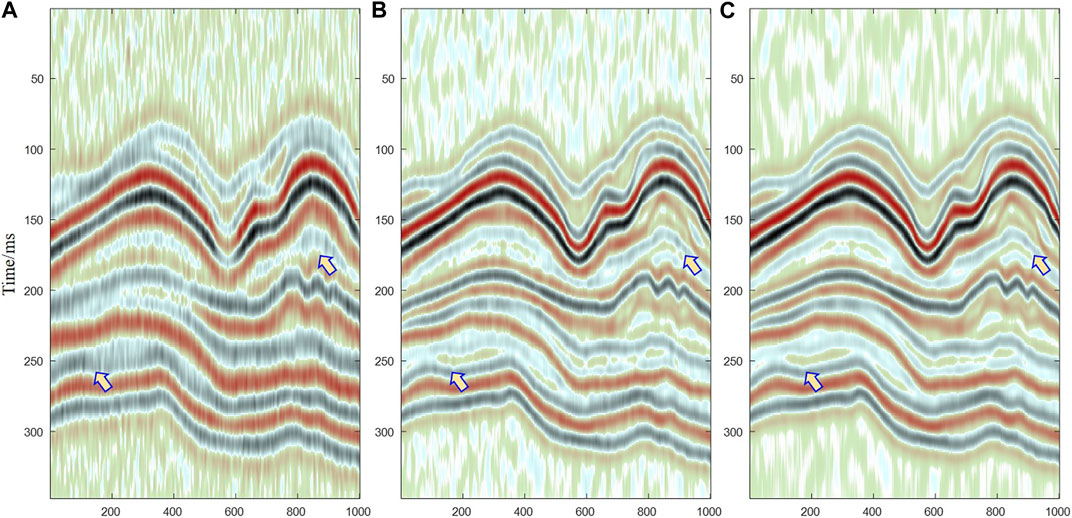
FIGURE 8. (A) Noise-containing seismic record; (B) High-resolution section by spectral modeling method; (C) High-resolution section by the proposed method.
4 Example
4.1 Applications in thin reservoir and microstructure recovery
For testing, 3D seismic data from the GST area of the Sichuan Basin was utilized. The targeted stratum is the Qixia Formation, and its thickness remains relatively stable at approximately 110 m. The depth of the targeted stratum is 4,500–4,700 m. The reservoir type is a dolomite pore reservoir, characterized by low porosity and low permeability. The physical parameters of the reservoir are very similar to those of the surrounding rock. The reservoir thickness is thin, with each group of reservoirs ranging from 6 to 10 m in thickness. The dominant frequency of the seismic data is 25 Hz. The response of the reservoir within the Qixia Formation is disrupted by the strong reflection from the upper and lower boundaries of the targeted stratum. Low-resolution seismic data in the Sichuan Basin presents two primary challenges: firstly, it results in unclear seismic structural characteristics, and secondly, it obscures thin reservoir responses.
The reservoir of the Qixia Formation in the GST area of the Sichuan Basin is predominantly situated within the central portion of the targeted stratum. The forward geological model is designed to depend on reservoir characteristics, as shown in Figure 9A. The arrow points to the dolomite reservoir, which has a designed thickness of 10 m. The position of the reservoir gradually shifts from the left to the right, moving toward the center of the targeted stratum. The seismic forward data is shown in Figure 9B. The forward simulation process (from the geological model to the seismic record) uses the theory of the Zoeppritz equation. The dominant frequency of the seismic wavelet is 35 Hz. It can be observed that the reservoir exhibits a strong bright spot response when it is located near the center of the targeted stratum. The bright spot response of the reservoir gradually weakens as it approaches the upper boundary of the targeted stratum. The forward model test shows that the presence of a reservoir leads to a bright spot response within the targeted stratum. However, in practice, the bright spot response of thin reservoirs may not be readily apparent due to limitations in the resolution and signal-to-noise ratio of seismic data. High-resolution seismic data is essential for accurately predicting the presence of thin reservoirs.
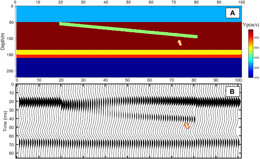
FIGURE 9. Seismic forward simulation. (A) Designed geological model with the reservoir in the middle of targeted stratum; (B) Seismic forward section by the Zoeppritz equation.
Figure 10 illustrates a comparison of the efficacy of different methods on real seismic data. Figure 10A shows the original seismic section. There are two industrial gas wells named Well 1 and Well 2, but there is no bright spot response from the reservoir at Well 1. This is primarily due to the scarcity of seismic data, leading to an extended duration of the wavelet. The identification of the reservoir is challenging due to the obstruction caused by the side lobes of the seismic-reflected wavelets at the top and bottom. Simultaneously, the stratum contact (P1m) consists of low-speed argillaceous limestone above and high-speed limestone below. It is observed as a peak response on the seismic section. Nevertheless, the presence of seismic noise and constraints in frequency ranges, combined with the impact of intricate lithological formations in the upper section of the targeted stratum, result in the overlapping of seismic wavelets from different reflection interfaces. Consequently, it is not feasible to precisely track the position of the stratum. Hence, the interpretation of the P1m strata (as shown in Figure 10A, at position ③) presents a challenging task. Two methods are employed to improve the resolution of seismic data in order to address this issue. Figure 10B shows the effects of spectral modeling deconvolution with spatial continuity constraints. It can be seen that the resolution of seismic data is effectively improved, particularly in the vicinity of the reservoir (Figure 10B, at positions ① and ②). The bright spot response of the reservoir is very clear. However, there is a sudden increase or decrease in the energy level at the upper boundary of the targeted stratum (P1m), and the continuity of the stratum deteriorates, as shown at the circled position in Figure 10B (③). The primary factor is that the upper part of the targeted stratum contains a complex combination of lithologies. Furthermore, a flaw exists in the approach employed to retrieve the energy of the reflection interface, leading to an impact on the seismic reflection within the upper portion of the targeted stratum and causing a disruption in the energy convergence of P1m. Figure 10C shows the application effect of the proposed method. The reservoir is also clearly highlighted, and the bright spot response corresponds more accurately to the industrial gas wells. The convergence of the formation interface (P1m) energy and the interpretation of the structure becomes easier. The interpretation results are consistent with the principles of geology and logging.
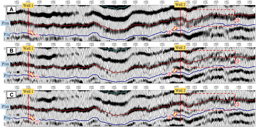
FIGURE 10. Sections comparison of different methods. (A) Original seismic section; (B) Seismic section by spectral modeling deconvolution with spatial continuity constraints; (C) Seismic section by the proposed method.
To confirm the precision of the high-resolution data, synthetic records from the two wells depicted in Figure 10 were utilized to compare with the processed data near the same wells. Figure 11A shows the logging data from Well 1 and its synthetic seismic record with a wavelet of dominant frequency 35 Hz. The high-resolution data obtained through the conventional spectral modeling approach and the novel method introduced in this paper were extracted in close proximity to the well in order to be compared with the synthetic seismic record, as shown in Figure 11A (3) and (4), respectively. The waveforms of both methods closely resemble the synthetic record at the targeted stratum position, and both methods exhibit a strong response from the reservoir. However, in the upper portion of the targeted stratum, the spectral modeling method does not match well with the synthetic record in terms of the time-shift and amplitude bias. The correlation coefficient of the method proposed in this paper is 0.71. While the waveform recovery method in this paper is more accurate and better matched with the synthetic record, and its correlation coefficient reaches 0.85. Figure 11B shows the synthetic record of Well 2 and the comparison of high-resolution seismic data near the well. It can be observed that the waveform generated by the traditional method in the targeted stratum poorly matches the synthetic seismic record, especially in stratum contact (P1m) where a significant time shift is evident. While the method described in this paper can accurately capture the reservoir information. The seismic stratum and the interpreted logging stratum correspond better.
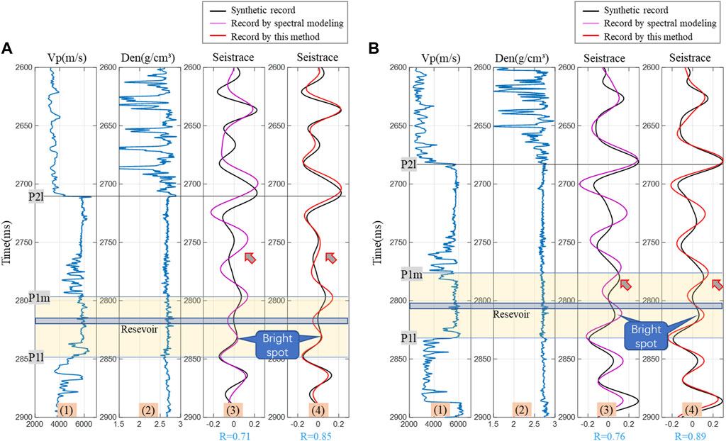
FIGURE 11. Well-to-seismic comparison. (A) P-wave velocity of Well 1 (1), density of Well 1 (2), synthetic seismic record with a wavelet of dominant frequency 35 Hz (black line in (3) (4)), high-resolution seismic trace by the traditional spectral modeling (pink line in (3)), and high-resolution seismic trace by the method in this paper (red line in (4)); (B) P-wave velocity of Well 2 (1), density of Well 2 (2), synthetic seismic record with a wavelet of dominant frequency 35 Hz (black line in (3) (4)), high-resolution seismic trace by the conventional spectral modeling (pink line in (3)), and high-resolution seismic trace by the method in this paper (red line in (4)).
According to the correspondence of the bright spot response to the reservoir, seismic bright spot responses indicate the presence of reservoirs. We selected a time window of 8 milliseconds below the upper boundary and 8 milliseconds above the lower boundary of the targeted stratum in Figure 10. The maximum peak amplitude in the time window is then extracted from various seismic data, as shown in Figure 12. Figure 12A shows the amplitude property extracted from the original seismic data. The bright spot response is not visible at Well 1, and there is a weak bright spot response at Well 2. In Figure 12B, the amplitude property extracted using the spectral modeling method with a spatial continuity constraint is shown. The bright spot response at Well 1 is enhanced, and a new bright spot appears at Well 2. But in the southern area (indicated by the white dashed line), there is a structural interpretation error caused by the absence of energy convergence at the upper boundary of the targeted stratum. This error leads to the occurrence of false bright spots and an unclear pattern. Figure 12C shows the amplitude property extracted from the data processed using the method described in this paper. The bright spot response is observed in Well 1 and Well 2, which is consistent with the forward analysis and logging interpretation. The explanation of the lower right corner of the figure is accurate, and the regularity of the highlighted amplitude is stronger.
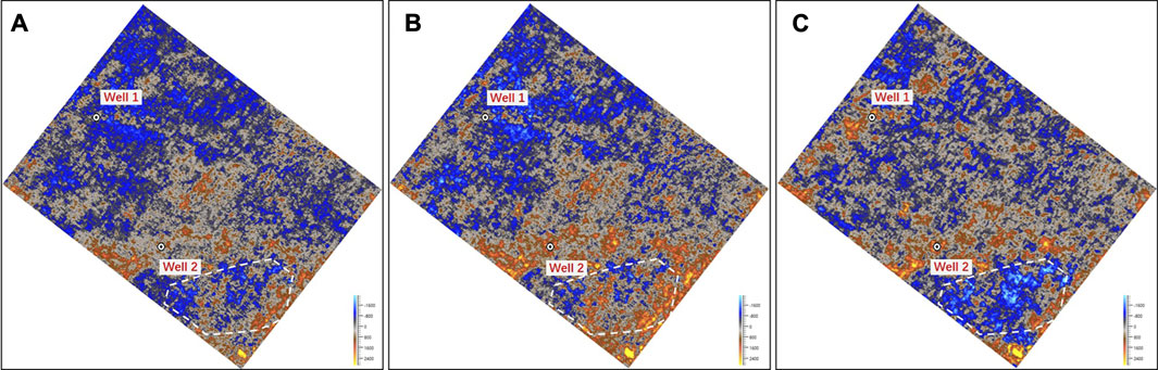
FIGURE 12. Maximum peak amplitude inside the targeted stratum extracted from different data. (A) Amplitude property from original seismic data; (B) Amplitude property from the data processed by the spectral modeling method with spatial continuity constraint; (C) Amplitude property from the data processed by the proposed method.
4.2 Applications in minor fault identification
High-resolution seismic data also contributes positively to the detection of minor faults. To assess the effectiveness of this approach in identifying minor defects, a particular area within the SN district in the Sichuan Basin was chosen for evaluation. The work area is characterized by a syncline structure, with the east and west wings exhibiting upturned formations and faults. Reservoirs primarily consist of lithological formations and are located in the central part of the syncline. Minor faults in this area have significant implications for reservoir reconstruction. The characterization of minor faults provide a foundation for accurate reservoir prediction, but its imaging is blurred due to the low resolution of the seismic data. The dominant frequency of seismic data is approximately 26 Hz, which makes it difficult to detect minor faults. Figure 13A shows the original seismic section, which demonstrates poor seismic resolution. So, minor faults and micro-tectonic morphology are similar, making it difficult to accurately identify them, especially in the y1 area. Figure 13B shows the seismic section processed using the method described in this paper. The figure shows the internal section of the syncline. The minor fault shown in Figure 13B is precisely delineated, with clear indication of the fault’s orientation and angle of inclination. Currently, seismic data has identifiable minor fault breaks of approximately 8 milliseconds. Based on the velocity of around 4,000 m/s here, the identifiable minor fault break is approximately 16 m. This confirms the accurate identification ability of the proposed method.
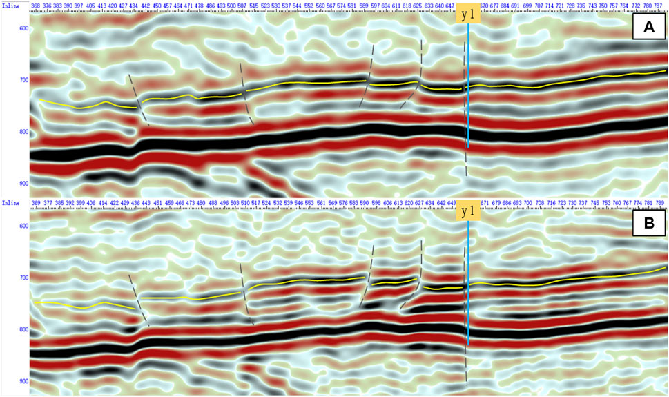
FIGURE 13. Seismic section comparison about minor fault. (A) Original seismic data with small obscure fault; (B) The high-resolution seismic section processed by the proposed method.
In light of these insights, the coherence property along the stratum interface was extracted, as shown in Figure 14. The faults on both sides of the work area developed, but the reservoir was primarily located in the syncline. So, the characterization of faults within the syncline was more significant, while micro-faults were indistinct within the syncline. Figure 14A shows the coherence map extracted from the original seismic data. The wells y1 and y2 in the work area are industrial gas wells, and the imaging logging shows that both wells have faults. There are faults in well y2, but no faults in well y1 on the original seismic coherence map. Figure 14B shows the coherence property of high-resolution data processed using the proposed method. The two wing faults can be clearly described, and the smaller faults are more visible within the syncline. The development of micro-faults can be clearly identified at well y1, which confirms the effectiveness of the proposed method in characterizing micro-faults.
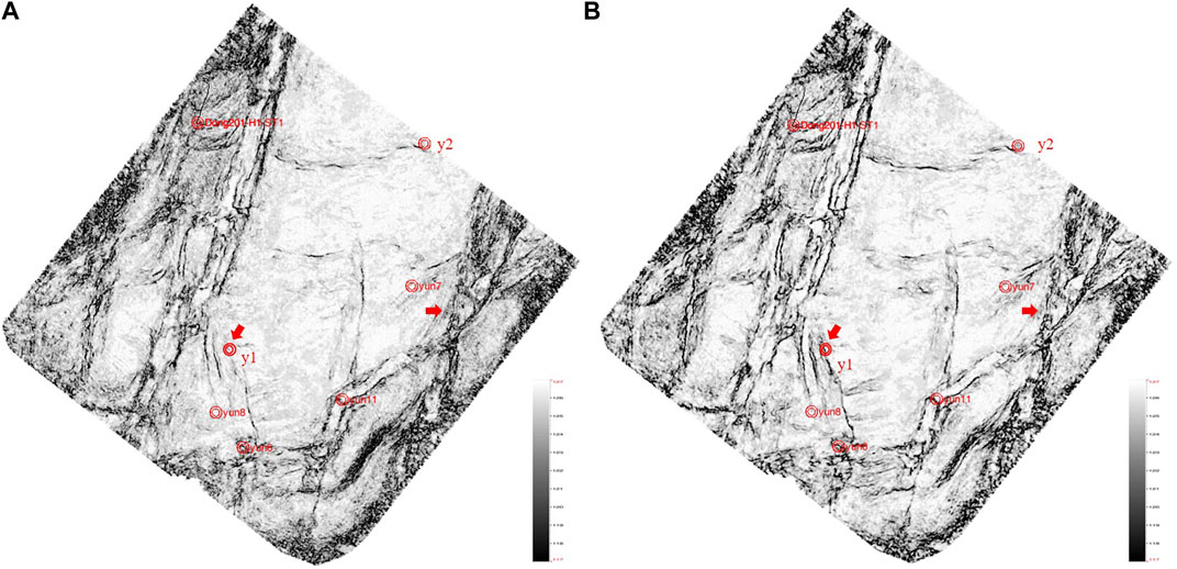
FIGURE 14. Coherence map of the targeted stratum comparison from different data. (A) Coherence map extracted from original seismic data; (B) Coherence map extracted from high-resolution seismic data processed by the proposed method.
5 Conclusion
In this paper, we propose a novel solution for extracting fine wavelets and recovering spatial structures through seismic spectral expansion, sparse reflection coefficient, and spatial continuity constraints. We conducted model trial calculations and processed actual data to validate the effectiveness and accuracy of the proposed method. Our findings indicate that the proposed method outperforms traditional methods such as spectral modeling deconvolution and sparse deconvolution. This study has led to significant conclusions and insights.
(1) In this paper, we construct the expected wavelet using spectrum scanning analysis and employ the frequency division fitting method. Then, by effectively expanding the frequency bandwidth, increasing the octave range, and improving the resolution of seismic data, we can achieve these enhancements while still adhering to the expected wavelet constraint. So, a precise wavelet and its corresponding high-resolution seismic data are accessible.
(2) The objective function for sparse deconvolution is formulated based on high-resolution seismic data and the expected wavelet. The seismic reflection coefficient can then be obtained. Meanwhile, the Hessian matrix regularization is used to constrain the spatial continuity of the seismic reflection coefficients. This method of regularization serves to safeguard the signal-to-noise ratio and accuracy of the seismic data.
(3) The final objective function is formulated by combining constraints on frequency expansion, sparsity, and spatial continuity. The high-resolution seismic data can be obtained without extracting the seismic wavelet. The proposed method is compared with traditional sparse deconvolution and spectral modeling deconvolution methods. The proposed method outperforms traditional methods in terms of noise suppression and enhancing the resolution capability of thin reservoirs.
Data availability statement
The raw data supporting the conclusion of this article will be made available by the authors, without undue reservation.
Author contributions
This paper was mainly completed by six authors. First, XG. completed the theoretical derivation and model testing. JGa. optimized the theoretical algorithm, and XY guided the theory derivation. SL worked on the model design. JGu provided suggestions for optimizing the theory. HW provided support for the actual production effect. All authors contributed to the article and approved the submitted version.
Funding
This work was supported by the Forward-looking and Fundamental Science and Technology Research Projects of PetroChina (2021DJ0606), the Basic Research and Strategic Reserve Technology Research Fund Project of Research Institutes Directly under Petrochina (2022D-XB01) and Major Science and Technology Special Project of GanSu Province (23ZDGA004).
Acknowledgments
The authors would like to thank the editors and reviewers for their valuable suggestions for this paper.
Conflict of interest
The authors declare that the research was conducted in the absence of any commercial or financial relationships that could be construed as a potential conflict of interest.
Publisher’s note
All claims expressed in this article are solely those of the authors and do not necessarily represent those of their affiliated organizations, or those of the publisher, the editors and the reviewers. Any product that may be evaluated in this article, or claim that may be made by its manufacturer, is not guaranteed or endorsed by the publisher.
References
Baziw, E., and Ulrych, T. J. (2006). Principle phase decomposition: a new concept in blind seismic deconvolution. IEEE Trans. Geoscience Remote Sens. 44 (8), 2271–2281. doi:10.1109/TGRS.2006.872137
Cabrera, E., Ronquillo, G., and Markov, A. (2020). Wavelet analysis for spectral inversion of seismic reflection data. J. Appl. Geophys. 177, 104034. doi:10.1016/j.jappgeo.2020.104034
Chen, F., and Zong, Z. (2022). PP-wave reflection coefficient in stress-induced anisotropic media and amplitude variation with incident angle and azimuth inversion. Geophysics 87 (6), C155–C172. doi:10.1190/geo2021-0706.1
Du, X., Li, G., Zhang, M., Li, H., Yang, W., and Wang, W. (2018). Multichannel band-controlled deconvolution based on a data-driven structural regularization. Geophysics 83 (3), R401–R411. doi:10.1190/geo2017-0516.1
Gholami, A., and Sacchi, D. (2012). A fast and automatic sparse deconvolution in the presence of outliers. IEEE Trans. Geoscience Remote Sens. 50 (10), 4105–4116. doi:10.1109/TGRS.2012.2189777
Gholami, A., and Sacchi, D. (2013). Fast 3D blind seismic deconvolution via constrained total variation and GCV. SIAM J. Imaging Sci. 6 (4), 2350–2369. doi:10.1137/130905009
Guo, T. C., Cao, W. J., and Tao, C. J. (2015). Research on time-varying spectral modeling deconvolution method. Geophys. Prospect. Petroleum 54 (1), 36–42. doi:10.3969/j.issn.1000-1441.2015.01.005
Guo, X., Gao, J. H., Yin, X. D., Yong, X. S., Wang, H. Q., and Li, S. J. (2022). Seismic high-resolution processing method based on spectral simulation and total variation regularization constraints. Appl. Geophys. 19 (1), 81–90. doi:10.1007/s11770-022-0927-5
Heimer, A., and Cohen, I. (2009). Multichannel seismic deconvolution using markov–Bernoulli random-field modeling. IEEE Trans. Geoscience Remote Sens. 47 (7), 2047–2058. doi:10.1109/TGRS.2008.2012348
Li, G. F., Qin, D. H., Peng, G. X., Yue, Y., and Zhai, T. L. (2013). Experimental analysis and application of sparsity constrained deconvolution. Appl. Geophys. 10 (2), 191–200. doi:10.1007/s11770-013-0377-1
Ma, X., Li, G., Li, H., and Wang, W. (2020). Multichannel absorption compensation with a data-driven structural regularization. Geophysics 85 (1), V71–V80. doi:10.1190/geo2019-0132.1
Macedo, D., Silva, D., Figueiredo, D., and Omoboya, B. (2016). Comparison between deterministic and statistical wavelet estimation methods through predictive deconvolution: seismic to well tie example from the North Sea. J. Appl. Geophys. 136, 298–314. doi:10.1016/j.jappgeo.2016.11.003
Mirko, V., and Pham, D. T. (2008). Robust wavelet estimation and blind deconvolution of noisy surface seismics. Geophysics 73 (5), 37–V46. doi:10.1190/1.2965028
Nasser, K., and Mauricio, D. (2014). Sparse multichannel blind deconvolution. Geophysics 79 (5), V143–V152. doi:10.1190/geo2013-0465.1
Rosa, A. L. R., and Ulrych, T. J. (1991). Processing via spectral modeling. Geophysics 56 (8), 1244–1251. doi:10.1190/1.1443144
Sacchi, M. D. (2010). Reweighting strategies in seismic deconvolution. Geophys. J. Int. 3, 651–656. doi:10.1111/j.1365-246X.1997.tb04500.x
Tang, B. W., Zhao, B., and Wu, Y. H. (2010). A new way to realize spectral modeling deconvolution. Oil Geophys. Prospect. 45 (S1), 66–70. doi:10.2118/154088-MS
Taylor, H. L., Banks, S. C., and McCoy, J. F. (1979). Deconvolution with the ℓ1 norm. Geophysics 44 (1), 39–52. doi:10.1190/1.1440921
Velis, D. R. (2008). Stochastic sparse-spike deconvolution. Geophysics 73 (1), R1–R9. doi:10.1190/1.2790584
Wang, D. Y., Huang, J. P., Kong, X., Li, Z. C., and Wang, J. (2017). Improving the resolution of seismic traces based on the secondary time–frequency spectrum. Appl. Geophys. 14 (2), 236–246. doi:10.1007/s11770-017-0616-y
Yu, C., Wang, S., and Cheng, L. (2022). Application of high-resolution processing in seismic data based on an improved synchrosqueezing transform. Front. Earth Sci. 10, 956817. doi:10.3389/feart.2022.956817
Yuan, S., Wang, S. X., Ma, M., Ji, Y., and Deng, L. (2017). Sparse Bayesian learning-based time-variant deconvolution. IEEE Trans. Geoscience Remote Sens. 55 (11), 6182–6194. doi:10.1109/TGRS.2017.2722223
Keywords: high-resolution processing, Hessian matrix regularization, spectral fitting, sparse deconvolution, spatial continuity constraint
Citation: Guo X, Gao J, Yong X, Li S, Gui J and Wang H (2024) A novel high-resolution imaging method based on sparsity in the time domain and spectral fitting in the frequency domain. Front. Earth Sci. 12:1247554. doi: 10.3389/feart.2024.1247554
Received: 26 June 2023; Accepted: 12 February 2024;
Published: 06 March 2024.
Edited by:
Sanyi Yuan, China University of Petroleum, Beijing, ChinaReviewed by:
Zhaoyun Zong, China University of Petroleum (East China), ChinaHongling Chen, Xi’an Jiaotong University, China
Copyright © 2024 Guo, Gao, Yong, Li, Gui and Wang. This is an open-access article distributed under the terms of the Creative Commons Attribution License (CC BY). The use, distribution or reproduction in other forums is permitted, provided the original author(s) and the copyright owner(s) are credited and that the original publication in this journal is cited, in accordance with accepted academic practice. No use, distribution or reproduction is permitted which does not comply with these terms.
*Correspondence: Xin Guo, Z3VveGluenN5QDE2My5jb20=