Vertical profiles of temperature, wind, and turbulent fluxes across a deciduous forest over a slope observed with a UAV

To contribute to a better understanding of the dynamics of the atmosphere inside and above a forest, vertical profiles are flown with a remotely-controlled multicopter in the Steinkrug forest. This area is located over a slope in the Solling natural area in Lower Saxony (Germany), composed mostly of deciduous trees about 30 m tall. Fifteen vertical flights made near sunset between summer 2019 and spring 2020 were inspected from the surface to 100 m above ground level. These measurements provide information on the vertical structures of wind and temperature within and above the canopy, including the effects of shallow slope flows near the ground. Contrasting measurements downhill outside the forest were also made. The gathered data allow estimated profiles of the turbulent fluxes of sensible heat and momentum to be obtained by computing averages and fluctuations for layers of 5 m depth. A leaf area density profile in both leafy and leafless conditions could also be produced. The presence of a slope flow is inspected at both sites, and the applicability of existing theories is explored.

1 Introduction

Forests cover a substantial part of the land surface of the planet [31% according to FAO and UNEP (2020)], the main exceptions being warm and cold desert areas, savannahs, terrains at high elevations, or lands dedicated to extensive grazing and farming. They may be evergreen, deciduous, or a mixture of the two. Many forests are old and dense; some are used for wood farming and managed accordingly. While some forests are cleared to make room for agricultural and grazing fields, others arise from the abandonment of areas previously used for agriculture. There are also man-made forests, such as orchards, that may cover large extents of terrain.

Some characteristics of a forest are the tree species that are found in it, the distribution of heights and the spatial density of trees, the structure of the foliage, the presence of leaf litter, and the local topography. A very useful quantity to summarize the characteristics of the forest canopy is the leaf area density (LAD) as a function of height, LAD(z) (Wang and Jarvis, 1990), which indicates the amount of vegetated area for a unit of surface. This quantity is usually derived by means of a prescribed tree and forest model. The vertical integration of LAD(z) provides the leaf area index [LAI, Watson (1947)], a parameter used in many applications.

In the literature, forests have usually been treated as having a dense canopy (Norman and Campbell, 1989) whose top acts as a separation layer between the air below and above it. Therefore, a particular within-canopy layer exists that behaves differently from the atmospheric boundary layer (ABL) that can be found in non-forested areas. If the canopy density is high, the top of the forest may be conceived as an elevated ground with its own thermal and roughness characteristics, considered porous as it allows some momentum, heat, and mass exchanges between the atmosphere above and inside the canopy (Belcher et al., 2012).

A dense canopy may exert a large drag on the wind, resulting in a much weaker wind under the canopy top (Patton and Finnigan, 2012). Furthermore, the top, usually with a low albedo, is heated by the Sun, and a convective ABL develops above the forest. Conversely, the stratification within the forest is stable, at least in its upper part, because there is warming at its top. The situation inverts at night if there is cooling at the top of the canopy as a stable ABL is formed above it, while the upper part of the canopy can become unstable (Jacobs et al., 1992) if the forest is considered compact. Near the surface, stability may depend on the presence of downslope flows if the terrain is not flat.

In dense canopies, the role of the forest surface is considered minor, especially if there is an isolating layer of dead leaf litter covering it (Wilson et al., 2000). This is a layer of a few centimeters of depth that, depending on the type of leaves, may act as a more or less efficient insulator of the exchange processes between the surface and the canopy atmosphere (Wilson et al., 2012). In the case of dense and deep leaf layers, the surface–atmosphere exchange may be small, and most of the diurnal cycle in the canopy is driven by the exchanges at the top of the canopy. The situation may change when a forest becomes leafless in winter. In the case of sparse and well-ventilated forests, this layer of dead leaves may not form.

However, there are other types of forests than those just described. If the forest is deciduous, it will lose the foliage in winter, and the roughness at the top, the LAD, and the thermal characteristics within the canopy will change dramatically as the top is no longer acting as a dense lid (Lu and Fitzjarrald, 1994). In this case, it is a matter of interest to see if the surface of the forest manages to connect with the atmosphere above, therefore eliminating the separated canopy sublayer.

In some areas with a Mediterranean climate, the natural vegetation may consist of perennial oak trees or similar species with a relatively low height and very variable tree density. These forests may have either a sparse distribution or a dense canopy. In the latter case, considering a continuous canopy as just described could be useful; otherwise, different strategies may be sought, either looking for the effects of individual trees (Dellwik et al., 2019) or of aggregations of trees (Garcia-Carreras et al., 2010).

Orchards, which are usually organized as lines of trees with free space between them, are a special case of tree agglomeration. In these cases, the interaction with the atmosphere above depends mostly on the direction of the wind and the sun’s rays with respect to the direction of the tree lines. This open canopy does not allow the establishment of a decoupled canopy layer from the atmosphere above, although the atmospheric conditions within the canopy are still different from those in non-forested areas (Dupont and Patton, 2012; Bailey and Stoll, 2013; Bailey, 2023).

The study of the vertical profiles of atmospheric variables and turbulence fluxes across a canopy and above has been made traditionally with towers taller than the canopy and instrumented at different levels. This approach allows for determining the evolution at the selected levels and performing long-term analyses that include the annual cycle and the multiannual evolution of the forest. Examples of such towers can be found in several locations, such as the Amazon Tall Tower Observatory (ATTO) in Brazil (Andreae et al., 2015), the Solling site in Germany (Constantin et al., 1998; Sogachev et al., 2011), the Russian-German installation in Siberia (Park et al., 2021), or some sites in the USA belonging to the National Ecological Observatory Network (NEON) and the AmeriFlux networks (Novick et al., 2018).

To complement the study of such forests, multicopter unmanned aerial vehicles (UAVs) allow exploring profiles obtained in a very short time (around 2 minutes) in wooded areas, as Cuxart et al. (2019) did by flying around and at the edge of a forested hill near Kassel in Germany. In recent years, multicopter UAVs have been used to investigate the stable boundary layer in polar regions (Kral et al., 2018), to explore the morning transition between land and sea breezes (Jimenez et al., 2016), or the evening transition over a river shore (Wrenger and Cuxart, 2017), usually by performing vertical profiles and horizontal transects. In this work, the technique has been applied to fly vertically inside the canopy and across its top in such a manner that detailed vertical profiles can be inspected and estimates of the turbulent variances and covariances can be obtained through spatial averaging over vertical layers. The flexibility of the system makes it possible to obtain similar profiles outside the forest near its edge shortly after those made within the forest, allowing comparisons between these locations.

The presence of significant topography in forested areas is an important factor. Upslope flows arise when the canopy top is warmer than the valley bottom; downslope flows arise when the opposite occurs. Their interaction with the canopy is still a subject of investigation (Aubinet et al., 2010; Xu et al., 2018). Furthermore, downslope flows may develop inside the canopy in leafless conditions at night, while they can be found in the daytime during the leafy season due to the thermal inversion in the canopy (Froelich and Schmid, 2006). It is an open question whether there could be shallow nocturnal downslope flows in the leafy period if the canopy is not compact enough, thus allowing for some surface nocturnal radiation cooling.

In this work, several vertical profiles of wind and temperature across and above the forest canopy are obtained with a fast-response sensor. Section 2 describes most of the methodological tools, which include the currently available theoretical framework relating the forest structure and the momentum exchange with the atmosphere, the sites where observations were taken, the sampling strategy, the measuring system, and the data processing. In Section 3, some of the selected profiles made in the early evening in leafy and leafless conditions are discussed in detail, together with those of a clearing nearby. This section also gives a preliminary estimation of instantaneous profiles of turbulent fluxes derived from spatially derived statistics taken from 5-m layers. Section 4 discusses some miscellaneous related subjects of interest, such as the details of the contrast between the leafy and the leafless canopies, the possibility of obtaining the profile of LAD from the friction velocity estimated by the measurements, and the description of downslope flows close to the ground in the forest and their interaction with the lower layers of the canopy. Finally, some conclusions are provided in Section 5.

2 Methodology

2.1 Available theories

The transport processes within a vegetation layer, such as a forest, are dominated by vertical momentum flux and dissipation of the turbulent kinetic energy. The drag created by the air flowing around the vegetation gives rise to gradients of the wind velocity. Information about the drag, the velocity gradients, and the momentum transfer can be deduced from the vertical profiles of wind, temperature, and Reynolds stress τ(z) (taken here as $\tau =-\rho \overline{u^{\prime }{w}^{\prime }}$). The density of the air is ρ; u is the component of the wind along its mean direction; v and w are the components perpendicular to u, with w being the vertical component for a flat forest; z is the height above ground level (agl); u′, v′, and w′ are the fluctuations of the wind components; and the overbar indicates a value averaged over time. According to Brunet (2020), the local equilibrium between the rate of momentum transfer along the mean direction and its rate of loss, assuming terrain homogeneity in the transversal direction, is given by

$-\rho \overline{u^{\prime }{w}^{\prime }}\left(z\right)=\rho c_D\left(z\right){\bar{u}}^2\left(z\right),(1)$

with the drag coefficient c_D(z). For the mean wind speed and the Reynolds stress, Brunet (2020) and Yi (2008) provide the equations

$\frac{d\left[c_d\left(z\right){\bar{u}}^2\left(z\right)\right]}{dz}=LAD\left(z\right)c_D\left(z\right){\bar{u}}^2\left(z\right)(2)$

and

$\frac{-d\overline{u^{\prime }{w}^{\prime }}\left(z\right)}{dz}+LAD\left(z\right)\overline{u^{\prime }{w}^{\prime }}\left(z\right)=0,(3)$

Thereby,

$LAD\left(z\right)=\frac{\frac{d\overline{u^{\prime }{w}^{\prime }}\left(z\right)}{dz}}{\overline{u^{\prime }{w}^{\prime }}\left(z\right)}(4)$

is the LAD as a function of the height agl. Eq. 4 and the following equations, except for Eqs 12, 14, are applied in the analysis of the experimental data. Let L(z) be the cumulative leaf area per unit ground area from ground level to height z:

$L\left(z\right)={\int }_0^{z}LAD\left(\widehat{z}\right)d\widehat{z}.(5)$

The solution for Eq. 3 is

$-\overline{u^{\prime }{w}^{\prime }}\left(z\right)/u_{*}^2\left(h\right)=e^{-\left[LAI-L\left(z\right)\right]}.(6)$

Here, we have used the top boundary conditions LAI = L(h), with the height of the canopy h. With

$u_{*}^2\left(z\right)=-\overline{u^{\prime }{w}^{\prime }}\left(z\right)(7)$

for the friction velocity, we get $u_{*}^2(h)=-\overline{u^{\prime }{w}^{\prime }}(h)$ at the top of the canopy and

$u_{*}^2\left(z\right)=u_{*}^2\left(h_{cr}\right)e^{L\left(z\right)}(8)$

with the friction velocity at the bottom of the canopy $u_{*}^2(z=h_{cr})$, which is the layer above the soil at which branches and leaves start and is labeled as z = h_cr (cf. Figure 4). From Eq. 8, the profile of the cumulative leaf area per unit ground area from the ground level to z can be deduced as

$L\left(z\right)=\ln \left(\frac{u_{*}^2\left(z\right)}{u_{*}^2\left(h_{cr}\right)}\right).(9)$

The boundary conditions at the top h and the bottom of the canopy are related by

$-\overline{u^{\prime }{w}^{\prime }}\left(h\right)=-\overline{u^{\prime }{w}^{\prime }}\left(h_{cr}\right)e^{\mathit{LAI}}.(10)$

The mean wind speed can be obtained by integrating Eq. 2, resulting in

$\bar{u}\left(z\right)={\bar{u}}_h{\left[\frac{c_D^h}{c_D\left(z\right)}\right]}^{\frac{1}{2}}{e}^{-0.5*\left[LAI-L\left(z\right)\right]},(11)$

with the drag coefficient $c_D^h$ at the top of the canopy. According to Yi (2008), the minimum wind speed is located around the maximum canopy drag level, and a stably stratified layer might form around the maximum drag level if the potential temperature gradient is significant. Above the layer is a vertical exchange zone where vertical turbulent mixing dominates, and the region below is characterized by prevailing horizontal advection.

For a forest located on a slope, the gravity effect resulting in drainage flows must be considered. For steady-state conditions, the flows can be described by (Mahrt, 1982; Yi et al., 2005)

$-\frac{\partial \overline{u^{\prime }{w}^{\prime }}}{\partial z}-g\frac{\mathrm{\Delta }\theta \left(z\right)}{{\theta }_0}sin\alpha =c_D\left(z\right)LAD\left(z\right){\bar{u}}^2\left(z\right).(12)$

Here, θ₀ is the ambient potential temperature, and $\mathrm{\Delta }\theta (z)=\bar{\theta }(z)-{\theta }_0$ is the deficit of the potential temperature in the drainage flow with $\bar{\theta }(z)$ being the mean potential temperature profile in the drainage flow, and α is the angle of the slope initiating the drainage flow. Substituting the drag coefficient within the canopy, we obtain (Mahrt et al., 2000)

$c_D\left(z\right)=\frac{u_{*}^2\left(z\right)}{{\bar{u}}^2\left(z\right)}(13)$

and the friction velocity (see Eq. 7) into Eq. 12 results in

$\frac{\partial \left(c_D\left(z\right){\bar{u}}^2\left(z\right)\right)}{\partial z}-c_D\left(z\right){\bar{u}}^2\left(z\right)LAD\left(z\right)=g\frac{\mathrm{\Delta }\theta \left(z\right)}{{\theta }_0}sin\alpha .(14)$

By multiplying with e^−L(z) and integrating from z to the height of the top of the canopy h, the mean windspeed $\bar{u}(z)$ is given by

$\bar{u}\left(z\right)=\sqrt{e^{-\left(LAI-L\left(z\right)\right)}\frac{c_D^h}{c_D\left(z\right)}{u}_h^2-g\frac{\mathrm{\Delta }\theta \left(z\right)\sin \alpha }{{\theta }_0{c}_D\left(z\right)}{\int }_z^h{e}^{-\left(L\left(z^{\prime }\right)-L\left(z\right)\right)}d{z}^{\prime }}\equiv \sqrt{u_{\mathit{forest}}^2+u_{\mathit{slope}}^2},(15)$

containing contributions of the forest and the slope. The algebraic sign of Eq. 15 can be negative for upslope flows, which is neglected because only downslope flows are considered in the present work. The use of the potential temperature profile allows considering at least partially the effects of thermal stratification in the momentum equation because we apply this term for the whole depth of the canopy layer, taking the maximum value of the profile as the reference potential temperature.

In summary, the UAV measurements of wind and temperature and the experimental estimates of the friction velocity allow comparing the observations with the above theory. The LAD profile produced can replace the use of a prescribed profile from a standardized forest model.

2.2 Description of the sites

The area of interest in the forest is on the eastern part of the Weser Valley near the city of Höxter (orange circle in Figure 1), at z ≈ 210 m above sea level and at z ≈ 120 m above the Weser River and its valley. From the bottom of the Weser Valley, the terrain ascends in a nearly continuous slope of about 10% to z ≈ 400 m above sea level. The direction of the main ascent is ESE. Most of the trees shown in Figure 1 are deciduous, mainly beech, with some oak and larch, while there are also some spruce conifer trees. Apart from the unpaved roads within the forest and some spaces with younger trees, the plant cover is relatively homogeneous, cf. Figure 1. The measurement site in the forest is indicated by a red circle in Figure 1. A meteorological station in the forest approximately 20 m from the red circle provides data about wind speed, air temperature at 2 m and 0.3 m, radiation, soil temperature, and humidity. As a complement to the measurement site in the forest, we chose an agricultural field that serves as a large forest clearing in the lower part of the slope. The blue rhombus in Figure 1 indicates the location of the measurement flights in the clearing. A digital elevation model (DEM), created using the structure-from-motion method (SfM), confirms the main direction and continuous slope. SfM is a photogrammetric approach using a sequence of overlapping 2D images to estimate and create a 3D model (Westoby et al., 2012). In our case, the UAV took images at approximately 300 positions evenly distributed over the area of interest from a height of roughly 50 m agl.

Figure 1

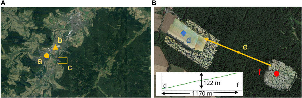
Figure 1. (A): Overview of the Weser Valley near Höxter (a, orange circle) and the Solling natural area, between the village of Fürstenberg (south) and the city of Holzminden (north). A SODAR is located at the bottom of the valley (b, orange triangle) and NW of the campaign site (c). The overview area has a dimension of approx. 25.5 km (W to E) by 12.8 km (N to S). (B) The UAV sounding locations are indicated by a blue rhombus for the open field (d) and a red circle for the forest site (f). The slope is indicated by the orange arrow (e) pointing downhill toward the WNW direction. The lighter green areas indicate the orthomosaic images that have been created by structure-from-motion photogrammetry (see text). The inset shows the slope, including the height difference of 122 m, for a distance of approximately 1,170 m between both sites. The area of interest has a dimension of approx. 1.5 km (W to E) by 1.0 km (N to S).

2.3 The measurement system

The multicopter Q17 used for the experiments consists of an airframe, a propulsion system, a rechargeable battery, avionics, telemetry, and a data acquisition system. The airframe is made of carbon fiber-reinforced plastics with a total weight of 0.75 kg, including folding arm mechanisms. Four electric engines with a total maximum power consumption of up to 4 kW are used to actuate the 16.8” propellers. During the flights of these experiments, a 4.5-Ah battery with a nominal voltage of 22.8 V provides power for at least three flights. Larger battery capacities of up to 16 Ah can be mounted but were not used for the experiments presented here to reduce the downwash effect created by the propellers. The multicopter system is controlled by a Pixhawk 2 autopilot¹ for the airborne part and a notebook PC running the QGroundControl² ground control station software. Both are connected by a bidirectional 433 MHz telemetry link. A second redundant telemetry and control system is provided by a 2.4-GHz RC transmitter and receiver. The height above ground level of the multicopter is provided by a pressure sensor, and the location is provided by the GPS sensor. An inertial measurement unit (IMU) provides the orientation and attitude of the UAV and usually consists of a combination of an acceleration sensor, a gyroscope, and a magnetometer. The IMU of the Pixhawk 2 additionally provides redundant magnetic, acceleration, and gyroscope sensors. The ground control station and the RC system both receive and display status information from the airborne system, thereby allowing the safety pilot and the ground control station operator to monitor the flights. Figure 2 shows the Q17 type multicopter and the TriSonica anemometer mounted on a 1-m-long rod that prevents the downwash from influencing the anemometer data. The amount of the downwash depends on several factors, including, for example, the mass of the UAV and the size of the propellers. Therefore, we fly with a small and light battery to reduce mass. The length of the carbon tube has been chosen to minimize and eliminate the vertical wind speed facing downwards in indoor, non-wind situations.

Figure 2

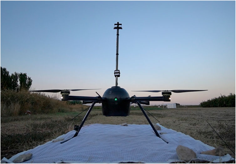
Figure 2. Q17 multicopter and the TriSonica sonic anemometer mounted on a 1-m-long rod to prevent the propeller’s downwash from influencing the sonic data.

The data acquisition system is not connected to the aviation system, and all relevant sensors are included in the setup. For the experiments, a Lightware SF11/C LiDAR³ is used both for the height above ground level and the vertical speed. The height data given by the LiDAR are more precise than data provided by pressure sensors and are not dependent on ambient temperatures. A TriSonica Mini weather station and 3D ultrasonic anemometer⁴ provide 3D wind, pressure, sonic temperature (denoted as T), and attitude data; an Adafruit Ultimate GPS⁵ provide the 3D location data and the (UTC) time stamp. All sensors have a USB interface and are connected to a Raspberry Pi 3B⁶ that is powered by a 2.6-Ah power bar. The sampling frequency is 10 Hz for the LiDAR, the Trisonica Mini, and the GPS. The raw data are combined with a local relative time stamp and sent to the Raspberry Pi, which receives the data, combines them with an additional GPS time stamp, and stores them on the micro SD card of the Raspberry Pi for post-flight analysis. The autopilot stores its data on an additional micro SD card with 50 Hz for the relevant data sources, including the IMU. The autopilot’s IMU data are used as a reference for the TriSonica Mini’s attitude data. The resolutions/accuracies of the TriSonica Mini are $0.01\frac{m}{s}$/$0.2\frac{m}{s}$ for the wind speed, 1°/1° for the wind direction, and 0.01°C/2°C for the temperature⁷.

The flight pattern, which is a vertical profile for the experiments presented here, is planned with the ground control station software and uploaded to the multicopter. The effect of the downwash was additionally reduced by flying vertically into undisturbed air. The ascent typically took 1–2 min to be completed, with a vertical speed of approximately 0.8 m/s. Because the multicopter flies into its own downwash during a vertical descent, the data of the descending phase of the flights are discarded.

Some test flights were operated in close vicinity and downstream to the SODAR at the bottom of the valley to compare the Q17 wind profiles with another wind profiling instrument; see Figure 1. On 30 December 2019, the wind speed was moderate during the daytime with a prevailing direction of about 200°, see Figure 3. The vertical wind profile of the TriSonica sonic anemometer (green dots), which was nearly instantaneous (1 min in total at 14:22, taking about 5 s to sample each vertical interval), closely resembles the 10-min averaged profiles provided by the SODAR at 14:20 (red circles) and 14:30 (blue circles), even though this individual realization may well correspond to a fluctuation departing from the averaged values.

Figure 3

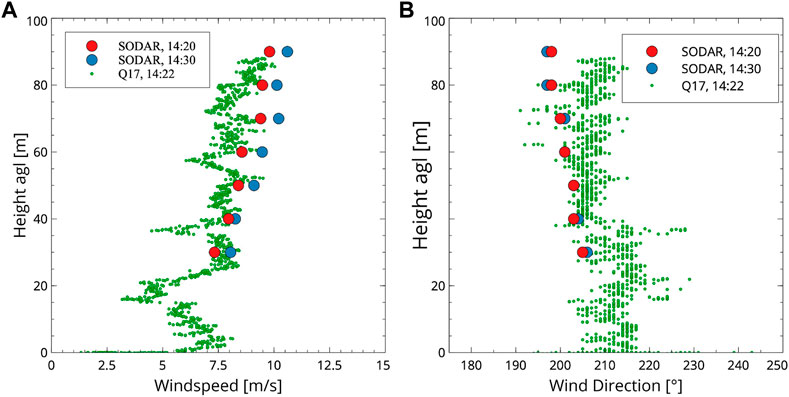
Figure 3. Inter-comparison of SODAR and Q17 wind speed (A) and direction (B). The small green circles represent the wind data, as sampled by the Q17 multicopter at 14:22 on 2019/12/30; the red and blue circles represent the SODAR data for 10-min time intervals at 14:20 and 14:30 on the same day. For this inter-comparison, the Q17 UAV was operated next to the SODAR.

2.4 Vertical structure of the forest

Several methods of estimating the leaf area density (LAD) have been proposed over the last two decades. Staebler and Fitzjarrald (2005) related the canopy structure and subcanopy flows, and the former is estimated based on measurements using an upward-looking laser range finder. Oshio et al. (2015) used multi-return airborne LiDAR data to estimate the LAD distribution of individual trees. Hosoi and Omasa (2006, 2007) used a 3D portable scanning LiDAR system to measure LAD, and Zhao et al. (2011) used a LiDAR system to analyze LAI, foliage profile, and stand height in forests. A different approach is described by Tang et al. (2016) as they investigated the LAI and vertical foliage profile using Landsat satellite images. The approach of the present paper assumes that the LAD of the forest in the vicinity of the meteorological station (close to the red circle in Figure 1) can be described by the LAD and the structure of an average prototype-like tree. The parameters of the prototype tree structure are derived from SfM and vertical profile measurements, as shown below.

The model of the prototype tree structure is based on the work by Grote (2003) and Grote and Reiter (2004). According to Grote and Reiter (2004), the shape (S_crown) can be described by

$S_{\mathit{crown}}\left(h_{\mathit{crown}}\right)=r_{\mathit{max}}\frac{\left(1-h_{\mathit{rel}}\left(h_{\mathit{crown}}\right)\right)*f\left(h_{\mathit{crown}}\right)}{\left(1-h_{\mathit{rel}}\left(h_{rmax}\right)\right)*f\left(h_{rmax}\right)}(16)$

with

$h_{\mathit{rel}}\left(h_{\mathit{crown}}\right)=\frac{h_{\mathit{crown}}-h_{cr}}{l_{cr}}(17)$

and

$f\left(h_{\mathit{crown}}\right)=b^{100*\left(h_{\mathit{crown}}-h_{cr}/l_{cr}^2\right)}.(18)$

h_crown is the height within the canopy. Figure 4A provides a sketch of a single tree and the parameters used in Eqs 16–18. r_max is the maximum radius of the crown of the tree at height $h_{r_{\mathit{max}}}$ and can either be deduced from the SfM analysis or taken from other references. h_cr denotes the height from ground level to the lower side of the canopy, and l_cr is the height of the canopy, i.e., the height of the tree is h_cr + l_cr. The function f(h) controls the size and shape of the tree structure as a function of the height h with h_cr ≤ h ≤ h_cr + l_cr. Its shape parameter b is responsible for the general shape of the prototype tree. Different tree species have different typical crown shapes, which are additionally influenced by the environment, including competition within a forest [see, e.g., Grote and Reiter (2004)]. A cone-shaped crown is obtained for b ≈ 1, and a strong concentration of the crown to the top of the trees is obtained for b ≈ 2. The latter shape is a good approximation for well-grown beech trees in competition with other trees in the close vicinity, and b ≈ 1.4 is a good approximation for trees with a crown with a nearly constant radius from the basis to the top of the crown. A 3D model of a part of the forest is created from SfM flights in a vertical plane, and b ≈ 2 is deduced in the vicinity of the measurement site in the forest (see Figure 1).

Figure 4

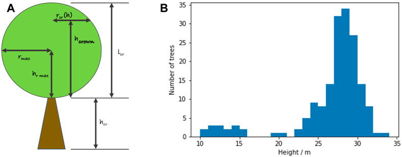
Figure 4. (A) Conceptual model of a tree; (B) observed distribution of tree heights at the forest site.

The size and shape of the trees in the area of interest must be analyzed to estimate the average leaf area. The DEM of the forest site provides information about the general structure, including the slope and the individual structures like trees, bushes, or forest tracks. The individual heights of 172 trees were analyzed to determine the average tree height in the vicinity of the forest site. The tree-height distribution histogram (see Figure 4B) indicates a narrow size distribution with a height of 28 m occurring most often. Therefore, the height of the canopy is set to h = 28 m for the remaining part of this paper.

Few trees are smaller than 15 m. Due to the analysis being conducted from above, bushes and smaller trees under the tree crown are not visible and have been analyzed from the vertical plane SfM data. The result is a superposition of essentially two stories of trees and foliage. This must be confirmed by the wind measurements (see below). As our SfM analysis cannot provide data about LAD, we assume LAD_max = 3.2 m²/m³ for beech trees according to Table 2 in Grote and Reiter (2004). In winter time, Simpraga et al. (2011) indicate that the LAI of beech in our altitude is $\approx 0.7m^2/m^2$, while it is $\approx 5m^2/m^2$ in summer (Grote and Reiter, 2004; Simpraga et al., 2011). Based on these data from the literature, we compute LAD(z) and L(z), assuming a vertical symmetry axis represented by the stem of the tree and a homogeneous distribution of the leaves and branches within the 3D structure described by the shape S_crown(z). From horizontal and vertical SfM analysis, we derive h_cr to be 0.8 times the height of the tree and r_max to be 0.2 times the height of the tree. For all the trees in the SfM analysis, the volume and position of the crown are computed and contribute to an averaged tree profile, which is thereby a superposition of the set of trees. According to Eq. 9, an L(z) profile can be obtained using the momentum flux profile obtained by the UAV, which can be compared with the prescribed profile of L(z) derived using Eqs 16–18. In Section 4.2, this is shown for the experimental results presented in Section 3.

2.5 Available profiles

Table 1 provides a list of the flights from August 2019 to April 2020. Profiles were made near sunset because downslope flows near the ground in leafless conditions start before sunset, and we were not authorized to fly later in the night. The table provides the date and time of the flight, the foliation status, and the time of sunset. The flights in and over the forest clearing were performed 15–30 min before or after the corresponding flight in the forest. This time gap was required to dismantle the UAV system at one of the sites, transport it to the next site, and set it up for the next flight.

Table 1

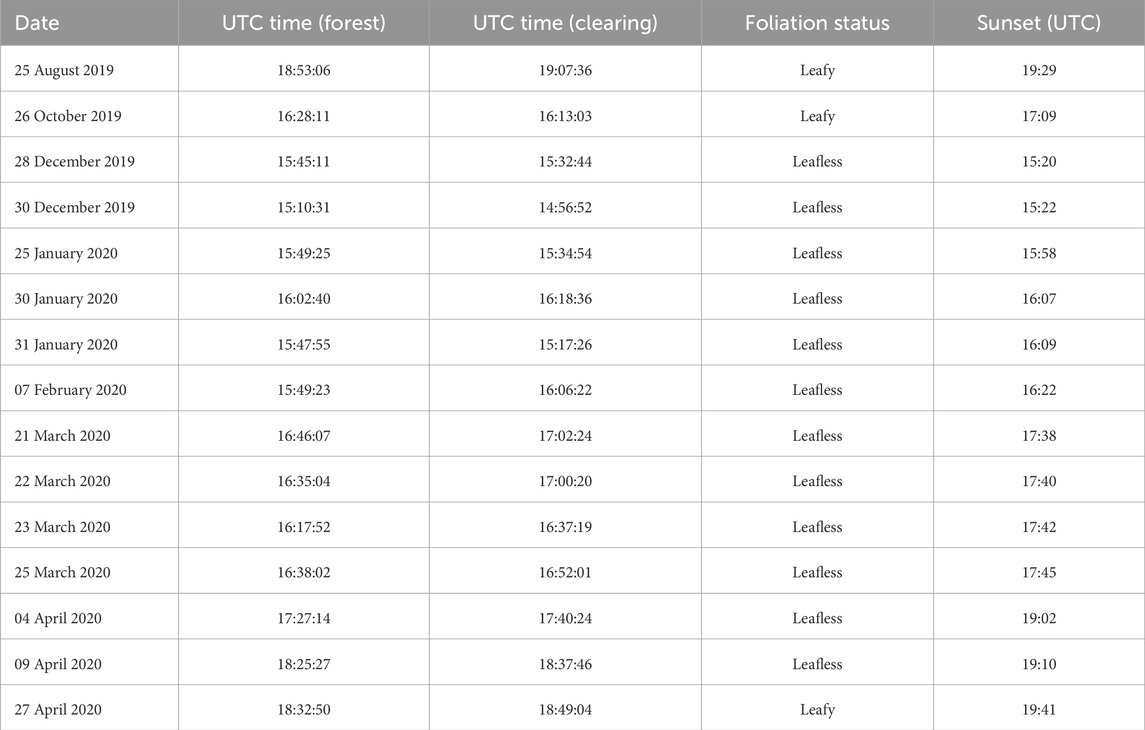
Table 1. List of sunset flights for the forest site used in this study showing the date and time of the start of the flights in the forest and in the clearing, the foliation status, and the UTC time of the sunset. Each flight took approx. 230 s.

During the leafy period of the year, the leaves lead to multipath and strongly damped GPS signals, making UAV flights more risky. Therefore, only three flights could be operated in leafy situations. They took place 36 min, 41 min, and 69 min before sunset in clear sky conditions with the upper canopy weakly illuminated. The twelve flights in the leafless period were made between 1.5 h before and 0.5 h after sunset, usually in clear sky conditions, with weak sunshine in the daytime corresponding to high latitude cold season conditions.

2.6 Data processing

The data analysis process reads the data sets created by the TriSonica sensor, the LiDAR distance sensor, and the GPS receiver. As the pressure data from the TriSonica sensor might be wrong due to cold temperatures and data from the LiDAR sensor could be incorrect due to multiple reflections from trees and the ground, both sensors’ data are fused and outliers are eliminated. The multicopter heading taken from the autopilot’s IMU and the heading of the TriSonica are used to compute the true heading. Invalid and incomplete data sets of the TriSonica instrument are usually characterized by very high wind speeds and/or very low temperatures. Therefore, wind speeds above a threshold of 20 m/s are replaced by the averaged values of the preceding and following data record. The same procedure is applied to temperatures below a threshold of T < − 8°C. These corrections are not applied to the ensemble of data analyzed in this work because wind speed is below 10 m/s and temperature is above 0°C in all cases.

As the vertical component of the wind is affected by the vertical movements of the multicopter, w is corrected with respect to the vertical speed. The data postprocessing also includes the incorporation of the movements of the multicopter, the removal of the descending part of the flight, and the computation of the profiles of temperature, wind, and the estimated turbulent fluxes. The main contribution of the movements of the multicopter is due to the ascent and descent. As mentioned above, a LiDAR range scanner is used to measure the distance from the multicopter to the ground, and its vertical speed v_v. v_v is subtracted from the vertical component w given by the Trisonica wind sensor. The descending part is not considered, as it is affected by the multicopter’s downwash. The results of this data processing procedure are vertical profiles for T, RH, and wind (u, v, w).

The turbulent fluxes are computed in the last step of the data postprocessing. For the fluxes, the averages of 5 m intervals are used as the multicopter is not stationary. For a 5 m interval, more than 60 samples contribute to the data of each interval. The fluctuations of wind speed and temperature are used to compute the sensible heat and momentum fluxes. For the following analysis, the averages and fluctuations are computed for the above-mentioned 5-m intervals. This strategy is a compromise. A sufficient vertical resolution for the estimations of the momentum and sonic temperature fluxes is needed to inspect their vertical changes in the canopy, and a resolution of 5 m allows recording at least six values in the canopy and a good resolution above it as well.

2.7 Preliminary evaluation and discussion of the data analysis

The values of the turbulent fluxes obtained from the fast-response sonic anemometer through the above-described procedure are nearly instantaneous profiles. Therefore, they are not directly comparable to fluxes obtained from time series at fixed points that are usually obtained from eddy-covariance systems installed in meteorological towers. We assume that in a complex environment like a forest canopy, the ergodic hypothesis, which states that both the time and the spatially derived statistics are equal to the ensemble values, is not valid.

Furthermore, while the standard deviation of the horizontal wind components and of the temperature are relatively small, about 0.5 m/s and 0.2 K, respectively, those of the vertical velocity are large, arising, for example, from the removal of the mean ascent velocity, which is considered constant during the averaging interval and the different flow conditions for the vertical axis of the sonic anemometer (if compared to the horizontal axis). This uncertainty translates into vertical turbulent fluxes that usually have uncertainties larger than 50%.

Therefore, the fluxes obtained here provide a short-term vision of the turbulent mixing, especially regarding eddies that may have characteristic times longer than the few seconds required by the UAV to fly a 5 m-layer upwards, and the interpretation of the profiles of the fluxes must take this into account. These lessons are applied when the system is used in subsequent experiments, and the flight ascents are slower so that the profiles obtained are more comparable to those obtained with time series in towers. However, in the present case, our after-the-fact approach has been to check if the obtained flux profiles display physical consistency with the profiles of temperature and wind and restrict interpretation to only those instances when this is effectively the case.

3 Description of some selected flights

The flights analyzed in this work have been made near sunset, with near-neutral thermal stratification above the forest. In consequence, the effect of the forest on the airflow above it is mostly through friction. The wind changes within the canopy due to the drag exerted by branches and leaves and usually displays stable thermal stratification as the ground surface is colder than the canopy top. These particular features will be described by examining some selected observed cases in this section.

Three non-neutrally stratified profiles in the interior of the forest will be discussed here to illustrate several features: i) the thermal effect of the canopy with foliage and of the leafless forest, ii) the presence of katabatic flows at the bottom of the forest, and iii) the consistency of the estimated turbulent fluxes with the observed wind and temperature profiles.

3.1 Late afternoon, leafy

A vertical profile was made across a leafy canopy in high-pressure conditions with WSW winds over the area on 27 April 2020, 45 min before sunset. As the forest is oriented to the west-north-west, it is illuminated by the Sun in the late afternoon, and the canopy top is a warm layer, although, at that time of the day, its longwave emission may exceed the incoming solar shortwave radiation.

The temperature profile averaged at a resolution of 5 m (c.f. Figure 5A, red circles) indicates that the temperature is at a maximum above the canopy top, having weakly unstable stratification above and very stable stratification below (of the order of 1K/10 m), although the stratification is less stable close to the ground (note that the canopy $\bar{\theta }$ profiles at 5-m resolution are displayed in Figure 9).

Figure 5

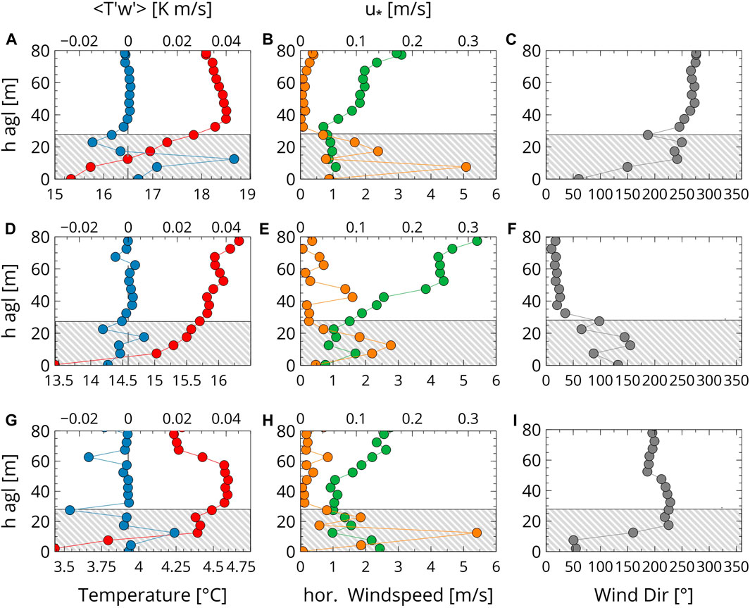
Figure 5. Profiles of T (red circles), $\overline{T^{\prime }{w}^{\prime }}$ (blue circles), horizontal windspeed (green circles), friction velocity u_* (orange circles), and direction of the wind (gray circles) at around sunset on 27 April 2020 (A–C), 9 April 2020 (D–F), and 28 December 2019 (G–I). The dashed gray vertical line in the left-hand part of the figures indicates $\overline{T^{\prime }{w}^{\prime }}=0$, and the shaded area indicates the forest up to the height of the canopy.

The estimated turbulent temperature fluxes (c.f. Figure 5A, blue circles) have signs and vertical profiles that are consistent with the temperature profiles. Above the canopy, there are very weak positive heat fluxes transporting heat upwards, while the upper canopy is stably stratified, with negative temperature fluxes. The negative high values under the canopy top may be related to the transport of warm air downwards (T′ > 0 and w′ < 0) through the porous top of the canopy (Belcher et al., 2012).

Two sublayers deserve specific comments. On one hand, close to the ground surface, the less stable layer appears to be related to the presence of a shallow downslope flow with small positive temperature flux values, as the surface is slightly warmer. On the other hand, there is a significant positive temperature flux in the layer 10–15 m agl, a finding that needs further exploration. This feature could be either due to a too-short sampling time or to the presence of the lower layer of trees and the top of the downslope flow, a layer for which positive occurrences of the sensible heat flux have been reported in stably stratified layers (Cuxart et al., 2020).

The wind speed (see Figure 5B, green circles) has values of 2 m/s well above the canopy and experiences a decrease to 0.8 m/s as it approaches the canopy top. In the canopy, it is weak, varies significantly with height, and shows a local maximum close to the surface. The friction velocity is much larger inside the forest than above it and displays a secondary maximum just above the top of the lowest trees (15 m agl). There is an even larger value of u_* close to the surface consistent with the presence of a downslope flow, a feature that seems confirmed by the profile of the wind direction, which has winds of easterly component in the lowest layers compared to the westerlies in the upper canopy and above.

Therefore, for this profile, the thermal and dynamic structure of the atmosphere across the canopy observed with the UAV behaves according to the expectations, and the estimated turbulent fluxes are consistent with this structure. Furthermore, despite the presence of a leafy canopy, a well-formed downslope flow exists close to the surface and favors the exchange between the surface and the lowest part of the canopy atmosphere.

3.2 Late afternoon, leafless

Measurements for the leafless early spring case (9 April 2020, Figures 5D–F) were made with a high-pressure system centered on the North Sea that was causing northerly flow over our area of study. The flight was made 45 min before sunset. In this case, the absence of leaves means the late afternoon sunshine is essentially dispersed by the dense branch system $\left(\mathit{L},\mathit{A},\mathit{I},,\text{about},,0.7,\frac{m^2}{m^2}\right)$ and is mostly diffused when it reaches the ground.

The wind is about 4 m/s well above the forest (see Figure 5E), decreasing to 2 m/s between 60 and 30 m agl and about 1 m/s in the leafless canopy. The wind direction is north above the canopy and easterly within (Figure 5F). The friction velocity above the canopy is larger than for the leafy case due to the larger velocity gradient here. At the canopy top, the friction velocity is smaller due to the lack of leaves, while at the bottom half, the dense branch system and the bushes produce significant drag. Near the surface, south-east winds of 2 m/s are compatible with the presence of a downslope flow, with values of u_* close to half of those of the leafy case.

The temperature profile (Figure 5D) shows a well-mixed layer immediately above the canopy top and a weakly stratified layer immediately below it. It can be inferred that the former is likely linked to the mechanical mixing induced by the wind shear, whereas the one in the upper half of the canopy is probably well connected with the layer above and cooler due to the shadow effect of the branches. The temperature fluxes are positive above the canopy top and negative under it, indicating heat transportation in both directions from this layer. Again, a positive value of the temperature flux is found at the layer of the lower trees.

The lower half of the canopy is stably stratified as the solar radiation at this time of the day does not reach the ground in a direct manner, and the longwave radiation emitted from the surface can reach the free atmosphere in the absence of leaves, resulting in a negative radiation flux at the surface. The temperature flux (blue circles in Figure 5D) in this layer is negative, as expected for a stably stratified layer. Near the surface, the downslope flow enhances this negative flux as it brings warmer air downwards in a very stable environment.

3.3 Early night, leafless

This flight was made in the leafless forest 25 min after sunset (28 December 2019, see Figures 5G–I), in night-time conditions, when our area was in the center of a 1,040-hPa high-pressure system. The wind above the canopy during the flight was from the west-south-west and was weak, less than 3 m/s in the whole profile. Temperatures were low, around 4°C, slightly colder close to the surface.

While the temperature structure at the top of the canopy (Figure 5G, red circles) is very similar to the previous case (two well-mixed layers above and below the canopy top), the lower half is mostly determined by the presence of a strong (3 m/s) and relatively deep (10–15 m) flow near the surface (winds with an easterly component, north-east close to the surface and south-east just above), compatible with a downslope flow, as the wind speed is at a maximum close to the surface.

The upper canopy has the same wind direction as the wind above it, with a layer on top connecting to the flow above the forest. The upper branches exert significant drag, as shown by the high value of the friction velocity (Figure 5F, orange circles).

Closer to the ground, there is a large friction velocity value at the layer of the lower trees and stronger wind below. The stratification is strong, indicating that the downslope flow is not significantly turbulent because the temperature flux is very small, while at its top, there is a significant positive flux, as described for the leafy case.

This case illustrates that at night, for a leafless canopy on a slope, katabatic flows can develop well with intensities similar to those found over unforested terrain. It also highlights the importance of the dense branch system as a factor organizing turbulence within the canopy.

Some of the changes in the wind direction in Figures 5C, F, I seem to be very large. Nevertheless, they are assumed to represent the wind direction very well as they are averaged over approximately 60 samples.

4 Discussion

In this section, three different aspects of the flow in forest canopies over a slope will be inspected. First, the vertical structure of the wind and momentum flux across the canopy will be analyzed separately for the leafy and the leafless cases, considering the ensemble of available flights, all made at approximately the same time of the day, near sunset. Second, the characterization of the canopy structure using the obtained wind profiles will be explored. Finally, the contribution to the dynamics within the canopy of the downslope flows close to the surface will be explored for the three cases described in Section 3, taking advantage of the theory of Yi et al. (2005) described in Section 2.

4.1 Contrasting leafy and leafless measurements

In order to see if the indications given by the individual cases described in the previous subsection on the wind structure and the friction velocity can be generalized, we analyze separately the averages obtained from the three leafy and the twelve leafless profiles. Furthermore, we take the chance to contrast these profiles with the averages on the large clearing downhill in order to obtain further insights into the processes taking place. In all cases, the height has been divided by 28 m, the most common tree height, which provides the reference height z/h = 1.0. Figure 6 shows windspeed and u_* for the forest site (first row) and the forest clearing (second row). The non-dimensionality of windspeed and friction velocity is a consequence of the normalization by the maximum values prior to the averaging.

Figure 6

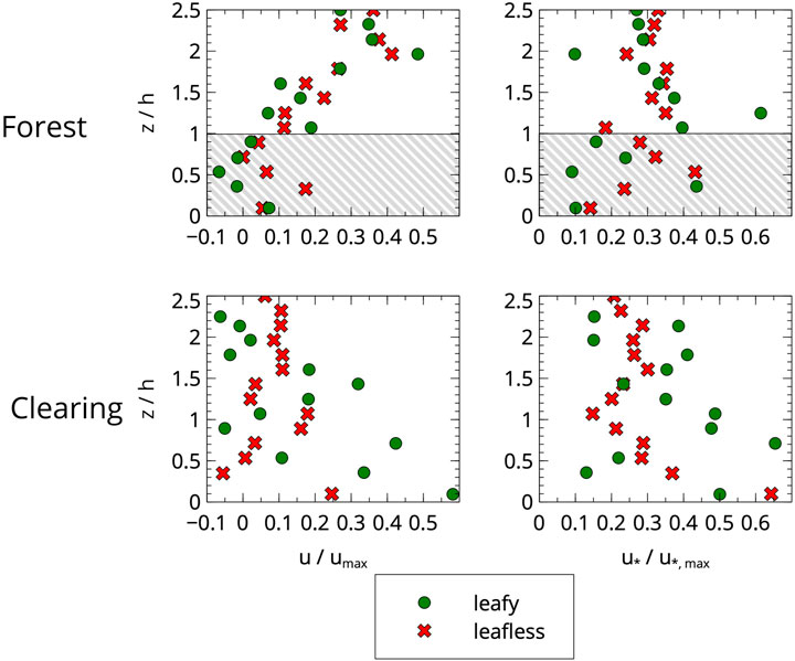
Figure 6. Averaged profiles of wind speed (left) and u_* (right, computed using Eq. 7). First row: across a leafy forest with the shaded area indicating the average top of the canopy; second row: clearing downhill of the forest. The red crosses refer to the leafless period, and the green circles, to the leafy period.

4.1.1 Leafy forest

The three profiles were made at very different times of the year (April, August, and October) in the late afternoon, 70 min, 36 min, and 41 min before sunset (green circles in Figure 6). The average windspeed profile in the leafy forest near sunset shows a speed decrease from above until the top of the canopy, with a maximum of the friction velocity in this layer. In the upper canopy, the wind and the velocity friction are smaller, essentially acting as a decoupling layer, while a downslope wind appears near the surface with significant mixing at its top. Therefore, the characteristics that appeared in the analysis of the individual profiles in the previous subsection seem to be confirmed when looking at the average of the three available flights.

In the clearing (green circles in Figure 6, lower row), the windspeed minimum at z ≈ 0.9 h also separates two regimes, with the maximum average windspeed close to the ground and a second average windspeed for 0.9 h < z < 1.7 h. The maximum windspeed close to the ground is compatible with a downslope flow, here stronger than in the forest, indicating that the slope flow accelerates when leaving the forested area. The maximum turbulence takes place near the ground instead of at the top of the downslope flow. The secondary maximum at z ≈ 0.6 h may be related to the mixing caused by the edge effect of the flow above the forest as it suddenly blows over non-forested terrain. Ma et al. (2020) used large-eddy simulations to show that there is an acceleration of the flow at the forest edge corresponding to the intrusion of the upper air downstream when the forest ends.

4.1.2 Leafless forest

The 12 leafless cases provide a larger sample than the leafy cases, and the averages are probably more representative of the typical behavior. The flights were made between late December and early April, and all the flights were before sunset except 28 December, which was 25 min after sunset, as discussed in the previous section.

The behavior above the canopy is similar to the leafy case (red crosses in Figure 6), as the wind speed above the forest decreases as it approaches the top of the canopy. The wind speed decreases as we go deeper in the canopy, as in the leafy case, until $\approx 0.5h$, with a local maximum at z ≈ 0.25 h (nearing 7 m above the ground), compatible with a well-developed downslope flow. This conceptual view is supported by the profile of u_*, which indicates less friction at the top of the canopy than in the leafy case due to the lack of leaves and a maximum at the wind shear part above the downslope flow.

In the clearing, the downslope flow accelerates as for the leafy case, but the secondary maximum at z ≈ 0.6 h is missing, probably because the edge effect is much smaller when the forest is leafless.

4.1.3 Drag coefficient and standard deviation

The drag coefficient can be deduced from Eq. 13 based on friction velocity and wind speed. Figure 7A shows the profiles of c_D for the forest site with the maximum scaled to 1.0. c_D is similar for the leafy and the leafless case above z/h = 1. For z/h < 1, there is clearly a structure of two maxima in the leafy period, probably related to two levels of maximum leaf density, whereas the leafless period displays a maximum at the height where the branch density may be maximal. The non-dimensionality of c_D in this figure is again a consequence of the normalization by the maximum values prior to averaging. Figure 7B shows the standard deviation σ_W scaled by the friction velocity u_* for the leafy period (green circles) and the leafless period (red circles). Both are similar, with large values close to the ground due to the turbulence generated by the katabatic flow, with supplementary maxima for the leafy situation at z = 0.55 h, 0.9 h, and 1.95 h. σ_U shows a similar relationship (not shown). These diagnostics are consistent with the interpretation given in the previous subsection related to the vertical distribution of foliage and the presence of downslope flows, although there are inherent limitations in the method of computing the fluxes.

Figure 7

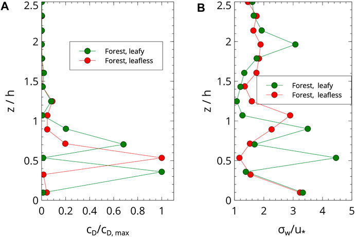
Figure 7. Contrasting averages of observed values (A) of c_D (computed using Eq. 11) and (B) σ_w for the leafy and the leafless forest. The maximum of c_D is scaled to 1.0.

4.2 Leaf area density estimated using momentum fluxes

Based on the data set described above and Eq. 4, the averaged LAD(z) and L(z) – as the integral of LAD(z)—can be computed as shown in Figure 8A for the forest site and leafy trees using the momentum flux profiles estimated with the UAV. The LAD computed with the momentum fluxes clearly detects a two-story situation in agreement with the observed structure of the forest shown in Figure 4B, specifically, the group of large trees with height h and maximum LAD at z ≈ 0.6 h and the understory with a maximum LAD at z < 0.2 h.

Figure 8

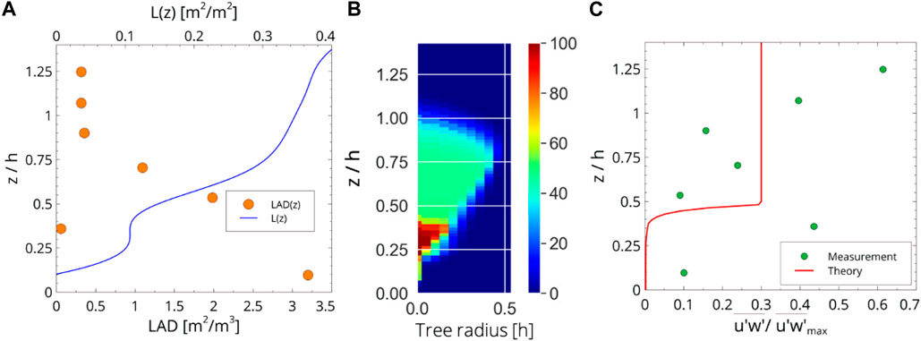
Figure 8. (A) Averaged leaf area density LAD(z) for the forest site and foliated trees, as derived from the measurements and L(z) as the integral of LAD(z). Based on the LAD shown here, a prototype tree structure of the forest can be deduced; see (B). The prototype forest is essentially a superposition of the large trees, the smaller trees, and the understory. The higher densities mean that more trees contribute to the LAD, as is the case for the younger trees below 15 m. (C) Momentum flux based on the measurements and the theory (using Eqs 7, 8), which is scaled to match the measured average momentum flux well above the canopy.

The heights of the trees shown in the histogram in Figure 4 are derived from a SfM analysis of images taken by the UAV in a horizontal survey pattern flight, cf. Section 2.4. The height, LAD(z) as shown in Figure 8A, and the conceptual tree model given in Eq. 16, taking b ≈ 2, are the basis for a prototype forest structure shown in Figure 8B for the forest site and foliated trees. The density in Figure 8B is a measure of the fraction of the trees contributing to LAD(z). As a consequence, the experimental data are able to provide suitable information about the average structure of the investigated forest.

In order to compare the measurement with data deduced from the structure of the forest described in Section 2.4, the derived momentum flux (Figure 8C) is computed based on Eq. 9 and the L(z) data shown in Figure 8A. The derived momentum flux is scaled to match the measured average momentum flux well above the canopy. The measurements reveal a small but non-vanishing momentum flux for z < 0.8 h [cf. 8 c)] and a larger value close to z/h = 0.3 located above the maximum of LAD(z) within the canopy. It increases for 0.8 h < z < 1.2 h and decreases from its maximum at z = 1.2 h up to z = 1.85 h. The momentum flux slowly decreases above z > 2 h. The model and the measurements show similarities from the ground to their respective maximums, but there are relevant differences: the estimated momentum flux does not vanish near the ground, which might be attributed to the usual presence of a downslope flow and the bushes and very small trees (c.f. Figure 4).

4.3 Downslope flows over the forest ground

The three individual flights discussed in Section 4.1 will be inspected here with respect to their accordance with the expression derived by Yi et al. (2005), cf. Eq. 15 for slope situations. The first term in Eq. 15, u_forest, shows that the wind in the canopy diminishes with respect to the value at its top as L(z) decreases approaching the surface. The term $c_D^h/c_D(z)$ also forces a decrease of speed, as approaching the surface, c_D(z) normally decreases with height for canopies with maximal LAD at their top. This will not be the case in our two-story layer, with the maximum of c_D(z) being found near 12 m agl, where the maximum branch density exists under a leafless upper canopy.

The second term in Eq. 15, u_slope, provides the contribution of denser air flowing downslope due essentially to the near-the-ground cooling and the slope angle, while the surface friction and the foliage oppose it. Because Δθ is negative close to the surface for downslope flows, the second term is positive in these conditions. To analyze the effect of this term, each individual flight takes θ₀ as the maximum value of the profile. In what follows, we assume that the momentum the fluxes obtained with the UAV are valid using the following-terrain coordinate system of Yi et al. (2005) because, with a slope angle of 10°, the projection would provide values not more different than 2%.

The leafy case of 27 April 2020 (Figure 9 upper row) has the largest c_D at the top, and the first term of Eq. 15 diminishes as the surface is approached as expected. Because the coldest part of the profile is near the surface, the second term of Eq. 15 generates a downslope flow in the canopy that is at a maximum near the ground. Therefore, the theory of Yi et al. (2005) seems to fit well with the observations for the leafy case.

Figure 9

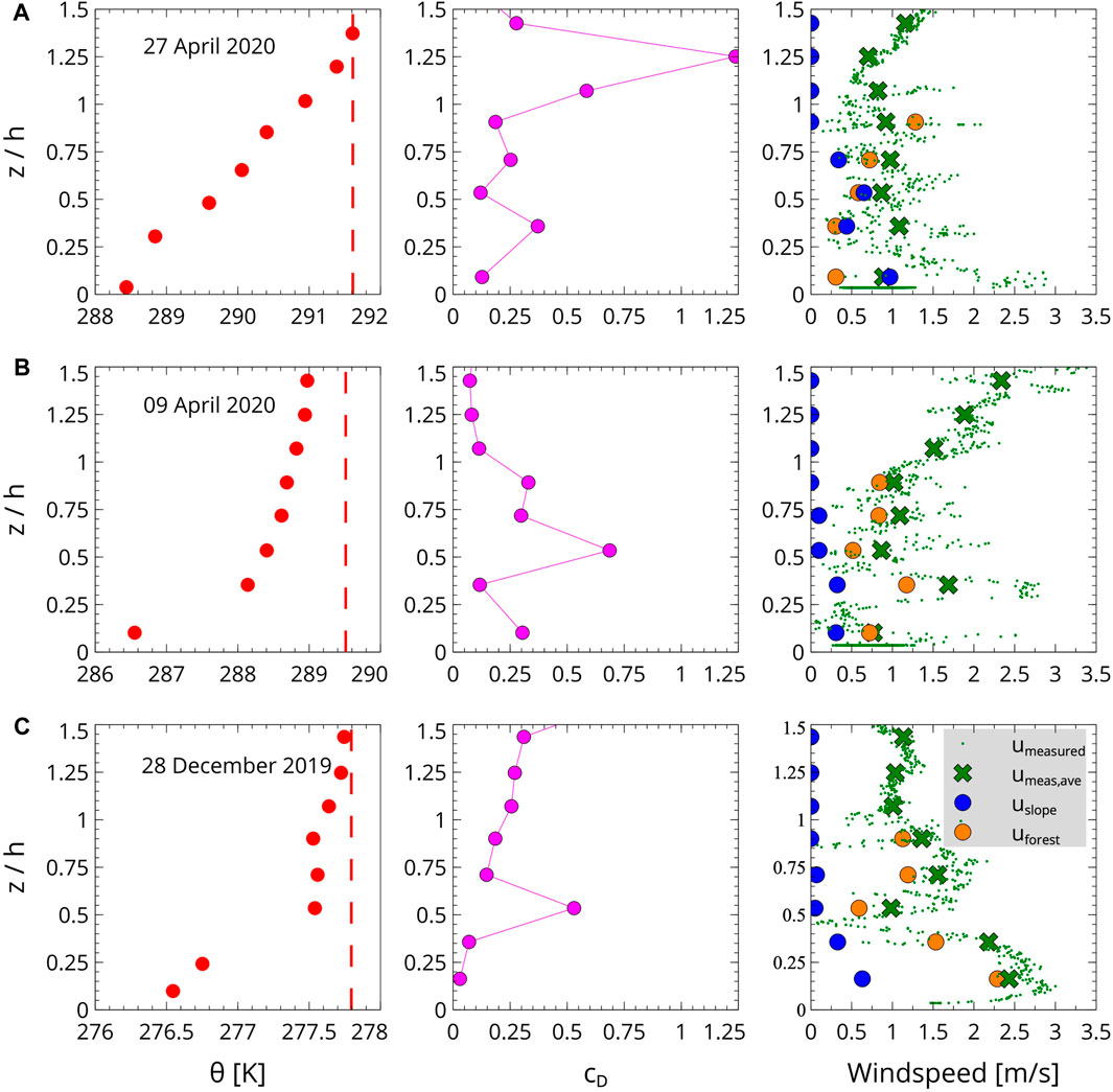
Figure 9. θ (red circles, left column), c_D (center column, magenta circles), and windspeed (right column) for (A) 27 April 2020, (B) 09 April 2020, and (C) 28 December 2019. The right column for the windspeed contains the measurements (small green circles), the averaged measurements (5-m intervals, green crosses), the slope part (blue circles), and the forest part (orange circles), according to Eq. 15. The dashed vertical line in the left column indicates the maximum θ value of the profile.

For the leafless cases, 9 April 2020 is 45 min before sunset (Figure 9 middle row), and 28 December 2019 is 25 min after it (Figure 9 lower row). In both cases, c_D(z) is maximal near 0.5 h, ≈14 m agl, corresponding to the maximal branch density within the leafless canopy, and the wind is at a minimum just above this height, with larger wind speed values under it, forecasted by the equation and seen in the observations.

The two leafless cases show more mixing in the upper part of the canopy than the leafy one, and the downslope flow is well-defined under the lowest branch layer, especially for the case after the sunset. Furthermore, Figure 9C right indicates that for the leafless case, the wind aloft can penetrate into the canopy according to the separation suggested by Eq. 15.

5 Conclusion

In this work, we have shown that it is possible to provide high-resolution profiles for temperature, wind speed, and wind direction in a dense deciduous forest. For the evening cases analyzed here, it is seen that the forest exerts a significant drag on the wind in both leafy and leafless conditions, while the wind decreases markedly in the 30-m layer above the canopy. The drag is at a maximum at the upper canopy and higher in the presence of leaves than in the leafless condition. Because the forest is located on a 10% slope, downslope flows develop and enhance mixing near the surface, more significantly in leafless conditions, when the forest is better connected with the atmosphere above it.

The measurements in a large clearing downhill indicate that the downslope flows accelerate as they come out from the forest, and turbulence is generated near the surface. In the case of a leafy forest, there is a secondary turbulence maximum higher up over the clearing, mostly likely due to the forest edge effect causing turbulence mixing downwind of it.

The temperature profiles are usually neutral above the canopy near sunset, as is the case for this data set. The within-canopy air is colder than the air above. This is because in the daytime, the canopy is shaded, and in leafy conditions, it is stably stratified as the warmest layer is near the canopy top. Three cases analyzed here have well-defined stable layers in the canopy that support this rationale. They also show that downslope flows may generate mixing near the ground in both leafy and leafless conditions, enhancing the coupling of the surface with the canopy atmosphere compared to forests over flat terrain.

The estimation of the turbulent fluxes is rough as the data sample is not large for each analyzed layer, but the patterns seem to be in good agreement with the profiles of the mean variables. Larger values of friction velocity are found where the wind shear is strong. The expected sign of the temperature flux is obtained; it is negative in stable stratification and positive in the unstable conditions above the canopy top. To increase confidence in the estimated values of the fluxes in future experiments, it is recommended to ascend more slowly and generate longer data series per layer.

The availability of momentum fluxes with height allows estimation of the LAD profile, which can be directly used in applications like numerical models of the atmosphere. The results show that assuming a logarithmic profile for the variables does not apply when the canopy has multiple stories. The method proposed in this paper, further tested for other canopy configurations, could be an option for estimating average leaf area density profiles using the corresponding ones of momentum fluxes, a higher sampling frequency, and an optimal flying strategy for each situation.

Data availability statement

The raw data supporting the conclusion of this article will be made available by the authors, without undue reservation.

Author contributions

BW: Data curation, Formal analysis, Investigation, Software, Writing–original draft, Writing–review and editing. JC: Conceptualization, Investigation, Methodology, Writing–original draft, Writing–review and editing.

Funding

The author(s) declare financial support was received for the research, authorship, and/or publication of this article. This work is part of of the research projects RTI2018-098693-B-C31 and PID2021-124006OB-I00 funded by MCIN/AEI/10.13039/501100011033 and by the European Regional Development Fund (ERDF A way of making Europe).

Acknowledgments

The authors thank B. Martí, D. Martínez-Villagrasa, and C. Langohr for their support with respect to the weather station in the close vicinity of the experimental site. Three reviewers contributed greatly to producing a more solid manuscript with their suggestions.

Conflict of interest

The authors declare that the research was conducted in the absence of any commercial or financial relationships that could be construed as a potential conflict of interest.

Publisher’s note

All claims expressed in this article are solely those of the authors and do not necessarily represent those of their affiliated organizations, or those of the publisher, the editors, and the reviewers. Any product that may be evaluated in this article, or claim that may be made by its manufacturer, is not guaranteed or endorsed by the publisher.

Footnotes

¹https://ardupilot.org/copter/index.html

²http://qgroundcontrol.com

³https://lightwarelidar.com/products/sf11-c-100-m

⁴https://anemoment.com

⁵https://www.adafruit.com/product/746

⁶https://www.raspberrypi.com

⁷https://anemoment.com/features/

References

Andreae, M. O., Acevedo, O. C., Araùjo, A., Artaxo, P., Barbosa, C. G., Barbosa, H. M. J., et al. (2015). The Amazon Tall Tower Observatory (ATTO): overview of pilot measurements on ecosystem ecology, meteorology, trace gases, and aerosols. Atmos. Chem. Phys. 15, 10723–10776. doi:10.5194/acp-15-10723-2015

CrossRef Full Text | Google Scholar

Aubinet, M., Feigenwinter, C., Heinesch, B., Bernhofer, C., Canepa, E., Lindroth, A., et al. (2010). Direct advection measurements do not help to solve the night-time CO₂ closure problem: evidence from three different forests. Agric. For. Meteorology 150, 655–664. doi:10.1016/j.agrformet.2010.01.016

CrossRef Full Text | Google Scholar

Bailey, B. N. (2023). Calculation of the shear length scale in sparce canopy flows: do sparse canopies follow mixing-layer scaling? Boundary-Layer Meteorol. 188, 1–10. doi:10.1007/s10546-023-00804-2

CrossRef Full Text | Google Scholar

Bailey, B. N., and Stoll, R. (2013). Turbulence in sparse, organized vegetative canopies: a large-eddy simulation study. Boundary-Layer Meteorol. 147, 369–400. doi:10.1007/s10546-012-9796-4

CrossRef Full Text | Google Scholar

Belcher, S., Harman, I. N., and Finnigan, J. J. (2012). The wind in the willows: flows in forest canopies in complex terrain. Annu. Rev. Fluid Mech. 44, 479–504. doi:10.1146/annurev-fluid-120710-101036

CrossRef Full Text | Google Scholar

Brunet, Y. (2020). Turbulent flow in plant canopies: historical perspective and overview. Bound. Layer. Meteorol. 177, 315–364. doi:10.1007/s10546-020-00560-7

CrossRef Full Text | Google Scholar

Constantin, J., Inclan, M. G., and Raschendorfer, M. (1998). The energy budget of a spruce forest: field measurements and comparison with the forest–land–atmosphere model (FLAME). J. hydrology 212, 22–35. doi:10.1016/s0022-1694(98)00199-1

CrossRef Full Text | Google Scholar

Cuxart, J., Martinez-Villagrasa, D., and Stiperski, I. (2020). Validation of a simple diagnostic relationship for downslope flows. Atmos. Sci. Lett. 21, e965. doi:10.1002/asl.965

PubMed Abstract | CrossRef Full Text | Google Scholar

Cuxart, J., Wrenger, B., Matjacic, B., and Mahrt, L. (2019). Spatial variability of the lower atmospheric boundary layer over hilly terrain as observed with an RPAS. Atmosphere 10, 715. doi:10.3390/atmos10110715

CrossRef Full Text | Google Scholar

Dellwik, E., an der Laan, M. P., Angelou, N., Mann, J., and Sogachev, A. (2019). Observed and modeled near-wake flow behind a solitary tree. Agric. For. Meteorology 265, 78–87. doi:10.1016/j.agrformet.2018.10.015

CrossRef Full Text | Google Scholar

Dupont, S., and Patton, E. G. (2012). Influence of stability and seasonal canopy changes on micrometeorology within and above an orchard canopy: the CHATS experiment. Agric. For. Meteorology 157, 11–29. doi:10.1016/j.agrformet.2012.01.011

CrossRef Full Text | Google Scholar

FAO and UNEP (2020). “The state of the world’s forests 2020,” in Forests, biodiversity and people (Rome: FAO and UNEP). doi:10.4060/ca8642en

CrossRef Full Text | Google Scholar

Froelich, N. J., and Schmid, H. P. (2006). Low divergence and density flows above and below a deciduous forest: Part II. below-canopy thermotopographic flows. Agric. For. Meteorology 138, 29–43. doi:10.1016/j.agrformet.2006.03.013

CrossRef Full Text | Google Scholar

Garcia-Carreras, L., Parker, D. J., Taylor, C. M., Reeves, C. E., and Murphy, J. G. (2010). Impact of mesoscale vegetation heterogeneities on the dynamical and thermodynamic properties of the planetary boundary layer. J. Geophys. Res. Atmos. 115. doi:10.1029/2009jd012811

CrossRef Full Text | Google Scholar

Grote, R. (2003). Estimation of crown radii and crown projection area from stem size and tree position. Ann. For. Sci. 60, 393–402. doi:10.1051/forest:2003031

CrossRef Full Text | Google Scholar

Grote, R., and Reiter, I. M. (2004). Competition-dependent modelling of foliage biomass in forest stands. Trees 18, 596–607. doi:10.1007/s00468-004-0352-9

CrossRef Full Text | Google Scholar

Hosoi, F., and Omasa, K. (2006). Voxel-based 3-D modeling of individual trees for estimating Leaf Area Density using high-resolution portable scanning lidar. IEEE Trans. Geoscience Remote Sens. 44, 3610–3618. doi:10.1109/tgrs.2006.881743

CrossRef Full Text | Google Scholar

Hosoi, F., and Omasa, K. (2007). Factors contributing to accuracy in the estimation of the woody canopy leaf area density profile using 3D portable lidar imaging. Hournal Exp. Bot. 58, 3463–3473. doi:10.1093/jxb/erm203

PubMed Abstract | CrossRef Full Text | Google Scholar

Jacobs, A. F. G., Boxel, J. H. V., and Shaw, R. H. (1992). The dependence of canopy layer turbulence on within-canopy thermal stratification. Agric. For. Meteorology 58, 247–256. doi:10.1016/0168-1923(92)90064-b

CrossRef Full Text | Google Scholar

Jimenez, M. A., Simó, G., Wrenger, B., Prtenjak, M. T., Guijarro, J. A., and Cuxart, J. (2016). Morning transition case between the land and the sea breeze regimes. Atmopsheric Res. 172, 95–108. doi:10.1016/j.atmosres.2015.12.019

CrossRef Full Text | Google Scholar

Kral, S. T., Reuder, J., Vihma, T., Suomi, I., O’Connor, E., Kouznetsov, R., et al. (2018). Innovative strategies for observations in the arctic atmospheric boundary layer (ISOBAR) – the Hailuoto 2017 campaign. Atmosphere 9, 268. doi:10.3390/atmos9070268

CrossRef Full Text | Google Scholar

Lu, C. H., and Fitzjarrald, D. R. (1994). Seasonal and diurnal variations of coherent structures over a deciduous forest. Boundary-Layer Meteorol. 69, 43–69. doi:10.1007/bf00713294

CrossRef Full Text | Google Scholar

Ma, Y., Liu, H., Liu, Z., Yi, C., and Lamb, B. (2020). Influence of forest-edge flows on scalar transport with different vertical distributions of foliage and scalar sources. Boundary-Layer Meteorol. 174, 99–117. doi:10.1007/s10546-019-00475-y

CrossRef Full Text | Google Scholar

Mahrt, L. (1982). Momentum balance of gravity flows. J. Atmos. Sci. 39, 2701–2711. doi:10.1175/1520-0469(1982)039<2701:mbogf>2.0.co;2

CrossRef Full Text | Google Scholar

Mahrt, L., Lee, X., Black, A., Neumann, H., and Staebler, R. M. (2000). Nocturnal mixing in a forest subcanopy. Agric. For. Meteorol. 101, 67–78. doi:10.1016/s0168-1923(99)00161-6

CrossRef Full Text | Google Scholar

Norman, J. M., and Campbell, G. S. (1989). “Canopy structure,” in Plant physiological ecology (Springer).

CrossRef Full Text | Google Scholar

Novick, K. A., Biederman, J. A., Desai, A. R., Litvak, M. E., Moore, D. J., Scott, R. L., et al. (2018). The AmeriFlux network: a coalition of the willing. Agric. For. Meteorology 249, 444–456. doi:10.1016/j.agrformet.2017.10.009

CrossRef Full Text | Google Scholar

Oshio, H., Asawa, T., Hoyano, A., and Miyasaka, S. (2015). Estimation of the leaf area density distribution of individual trees using high-resolution and multi-return airborne LiDAR data. Remote Sens. Environ. 166, 116–125. doi:10.1016/j.rse.2015.05.001

CrossRef Full Text | Google Scholar

Park, S. B., Knohl, A., Migliavacca, M., Thum, T., Vesala, T., Peltola, O., et al. (2021). Temperature control of spring CO₂ fluxes at a coniferous forest and a peat bog in central Siberia. Atmosphere 12, 984. doi:10.3390/atmos12080984

CrossRef Full Text | Google Scholar

Patton, E. G., and Finnigan, J. J. (2012). “Canopy turbulence,” in Handbook of environmental fluid dynamics (Boca Raton: CRC Press), 1.

Google Scholar

Simpraga, M., Verbeeck, H., Soubie, R., Heinesch, B., Jockheere, I., Laffineur, Q., et al. (2011). Seasonal variation of LAI in the footprint of a flux measurement tower. Starters het Bosonderzoek.

Google Scholar

Sogachev, A., Panferov, O., Ahrends, B., Doering, C., and Jørgensen, H. E. (2011). Numerical assessment of the effect of forest structure changes on CO₂ flux footprints for the flux tower in Solling, Germany. Agric. For. Meteorology 151, 746–754. doi:10.1016/j.agrformet.2010.10.010

CrossRef Full Text | Google Scholar

Staebler, R. M., and Fitzjarrald, D. R. (2005). Measuring canopy structure and the kinematics of subcanopy flows in two forests. J. Appl. Meteorology 44, 1161–1179. doi:10.1175/jam2265.1

CrossRef Full Text | Google Scholar

Tang, H., Ganguly, S., Zhang, G., Hofton, M. A., Nelson, R. F., and Dubayah, R. (2016). Characterizing leaf area index (LAI) and vertical foliage profile (VFP) over the United States. Biogeosciences 13, 239–252. doi:10.5194/bg-13-239-2016

CrossRef Full Text | Google Scholar

Wang, Y. P., and Jarvis, P. G. (1990). Description and validation of an array model - MAESTRO. Agric. For. Meteorology 51, 257–280. doi:10.1016/0168-1923(90)90112-j

CrossRef Full Text | Google Scholar

Watson, D. J. (1947). Comparative physiological studies on the growth of field crops: I. variation in net assimilation rate and leaf area between species and varieties, and within and between years. Ann. Bot. 11, 41–76. doi:10.1093/oxfordjournals.aob.a083148

CrossRef Full Text | Google Scholar

Westoby, M. J., Brasington, J., Hambrey, N. F., and Reynolds, J. M. (2012). ‘Structure-from-Motion’ photogrammetry: a low-cost, effective tool for geoscience applications. Geomorphology 179, 300–314. doi:10.1016/j.geomorph.2012.08.021

CrossRef Full Text | Google Scholar

Wilson, K. B., Hanson, P. J., and Baldocchi, D. D. (2000). Factors controlling evaporation and energy partitioning beneath a deciduous forest over an annual cycle. Agric. For. Meteorology 102, 83–103. doi:10.1016/s0168-1923(00)00124-6

CrossRef Full Text | Google Scholar

Wilson, T. B., Meyers, T. P., Kochendorfer, J., Anderson, M. C., and Heuer, M. (2012). The effect of soil surface litter residue on energy and carbon fluxes in a deciduous forest. Agric. For. Meteorology 161, 134–147. doi:10.1016/j.agrformet.2012.03.013

CrossRef Full Text | Google Scholar

Wrenger, B., and Cuxart, J. (2017). Evening transition by a river sampled using a remotely-piloted multicopter. Boundary-Layer Meteorol. 165, 535–543. doi:10.1007/s10546-017-0291-9

CrossRef Full Text | Google Scholar

Xu, X., Yi, C., Montagnani, L., and Kutter, E. (2018). Numerical study of the interplay between thermo-topographic slope flow and synoptic flow on canopy transport processes. Agric. For. Meteorology 255, 3–16. doi:10.1016/j.agrformet.2017.03.004

CrossRef Full Text | Google Scholar

Yi, C. (2008). Momentum transfer within canopies. J. Appl. Meteorology Climatol. 47, 262–275. doi:10.1175/2007jamc1667.1

CrossRef Full Text | Google Scholar

Yi, C., Monson, R. K., Zhai, Z., Anderson, D. E., Lamb, B., Allwine, G., et al. (2005). Modeling and measuring the nocturnal drainage flow in a high-elevation, subalpine forest with complex terrain. J. Geophys. Res. 110. doi:10.1029/2005jd006282

CrossRef Full Text | Google Scholar

Zhao, F., Yang, X., Schull, M. A., Román-Colón, M. O., Yao, T., Wang, Z., et al. (2011). Measuring effective leaf area index, foliage profile, and stand height in New England forest stands using a full-waveform ground-based lidar. Remote Sens. Environ. 115, 2954–2964. doi:10.1016/j.rse.2010.08.030

CrossRef Full Text | Google Scholar