
94% of researchers rate our articles as excellent or good
Learn more about the work of our research integrity team to safeguard the quality of each article we publish.
Find out more
ORIGINAL RESEARCH article
Front. Earth Sci., 12 May 2023
Sec. Hydrosphere
Volume 11 - 2023 | https://doi.org/10.3389/feart.2023.976227
 Baptiste Dafflon1*
 Emmanuel Léger1,2
 Nicola Falco1
 Haruko M. Wainwright1,4
 John Peterson1
 Jiancong Chen3
 Kenneth H. Williams1,5
 Susan S. Hubbard1,6
Evaluating the interactions between above- and below-ground processes is important to understand and quantify how ecosystems respond differently to atmospheric forcings and/or perturbations and how this depends on their intrinsic characteristics and heterogeneity. Improving such understanding is particularly needed in snow-impacted mountainous systems where the complexity in water and carbon storage and release arises from strong heterogeneity in meteorological forcing and terrain, vegetation and soil characteristics. This study investigates spatial and temporal interactions between terrain, soil moisture, and plant seasonal dynamics at the intra- and inter-annual scale along a 160 m long mountainous, non-forested hillslope-to-floodplain system in the upper East River Watershed in the upper Colorado River Basin. To this end, repeated UAV-based multi-spectral aerial imaging, ground-based soil electrical resistivity imaging, and soil moisture sensors were used to quantify the interactions between above and below-ground compartments. Results reveal significant soil-plant co-dynamics. The spatial variation and dynamics of soil water content and electrical conductivity, driven by topographic and soil intrinsic characteristics, correspond to distinct plant types, with highest plant productivity in convergent areas. Plant productivity in heavy snow years benefited from more water infiltration as well as a shallow groundwater table depth. In comparison, low snowpack years with an early first bare-ground date, which are linked to an early increase in plant greenness, imply a short period of saturated conditions that leads to lower average and maximum greenness values during the growing season. Overall, these results emphasize the strong impact of snowpack dynamics, and terrain and subsurface characteristics on the heterogeneity in plant type and seasonal dynamics.
Improving the predictive understanding of ecosystem dynamics in mountainous watersheds is critical because of their strong societal relevance, as well as to their high vulnerability to environmental change. Snow-impacted mountainous watersheds, often referred to as “water towers,” provide 60%–90% of water resources worldwide (Viviroli and Weingartner, 2008). Each watershed responds to variability in meteorological forcing, extreme weather, climate change, land-use change, fire and other perturbations, and in turn influences water resources management, energy production, agriculture, and terrestrial life and life quality. These meteorological events and perturbations are modulated by the complex interactions between vegetation, topography, and subsurface, and collectively influence the system’s cumulative hydro-biogeochemical response, including ecosystem carbon and water cycles and downgradient water quantity and quality.
Seasonally snow-covered mountainous watershed systems are particularly sensitive to changes in meteorological forcing (Seddon et al., 2016), because of their intrinsic properties, alternate states within the system (including snow-rain), and strong seasonal and sub-seasonal weather patterns (Ernakovich et al., 2014). The hydro-biogeochemical responses of these systems are influenced by the spatial and interannual variability in seasonal and sub-seasonal weather events, as well as by a general trend toward warmer winters (e.g., Hayhoe et al., 2007) and earlier spring warming and occurrence of snow-free conditions (e.g., Contosta et al., 2017). The consequences of these changes are multifold. Decreased snowpack results in lower albedo and thus increases in the absorption of solar radiation. Greater absorbance of short- and longwave radiation can increase the soil temperature and evapotranspiration and thus decrease soil moisture (Fyfe and Flato, 1999; Stewar, 2009; Rangwala et al., 2013). In water-limited systems, early snowmelt and early plant growth can lead to drought conditions, whereby plants become water- and nutrient-stressed later in the season (Sloat et al., 2015; Devadoss et al., 2020; Wainwright et al., 2020). In systems that are not water limited, early and warm springs can lead to an extended period of plant water uptake and an extended period of plant carbon uptake through photosynthesis if enough nutrients are available (e.g., Keenan and Riley, 2018). Warm winters and/or thick snowpack can maintain soil temperature well above 0°C for a long period of time, which favors belowground microbial activity and carbon and nitrogen cycling (e.g., Brooks et al., 2011; Brooks et al., 2011; Euskirchen et al., 2017). Changes in these processes can lead to changes in carbon fluxes and storage (Ernakovich et al., 2014), and potential changes in species composition and distribution over decadal time frames.
Complex mechanisms control the flow of water in the hillslope to floodplain continuum and its accessibility to plant (Fan et al., 2019). Soil moisture is generally controlled by a combination of surface and subsurface water flow from upstream locations, snowmelt and rain events on the hillslope itself, but also depend on subsurface hydraulic properties, and fluctuation in the stream stage for locations in the floodplain. Several studies have focused on the flow of water in hillslope-to-floodplain continuum (e.g., McGlynn and McDonnell, 2003; Inamdar and Mitchell, 2007; Lowry et al., 2010; Thayer et al., 2018; Webb et al., 2018; Tokunaga et al., 2019). There have been fewer studies investigating the occurrence and abundances of meadow plants as a function of their position and their access to water resources (Loheide II and Gorelick, 2007; Hammersmark et al., 2010; Lowry et al., 2010; Lowry et al., 2011; Devadoss et al., 2020). Lowry et al. (2011) investigated the groundwater controls on vegetation composition and patterning in a mountain meadow in the Sierra Nevada mountains of California. They found that the hydrologic niches of several vegetation communities were best described using the integral of water table depth above an oxygen stress depth threshold and below a water stress depth threshold. Looking at meadow covered hillslopes in the East River Watershed in the Upper Colorado River, Devadoss et al. (2020) identified spatial zones that have characteristic Normalized Difference Vegetation Index (NDVI) time series from satellite data, and found that each zone represents a set of similar snowmelt and plant dynamics that differ from other zones and that these zones are associated with key topographic features, plant species and soil moisture.
Quantifying the soil and plant hydro-biogeochemical responses to warm winters and/or early snow melt in natural ecosystems is particularly challenging because of the strong heterogeneity in plant, soil and terrain characteristics that all impact the surface water and energy distribution and exchange. A major difficulty is to capture the soil and vegetation states with spatial and temporal resolution sufficient to understand their interactions and how they depend on factors such as topography, plant type, and snowmelt dynamics. Studies investigating the spatial as well as the temporal variability in above- and below-ground characteristics at local scale have been rare (e.g., Dafflon et al., 2017; Rudolph et al., 2015; von Hebel et al., 2018). Rudolph et al. (2015) used electromagnetic induction measurements and multi-temporal satellite imagery methods to document a relationship between bulk soil electrical conductivity and leaf area index. They found that physical and chemical interactions between crops and subsoil in arable fields were responsible for the spatial and temporal variation of the crop performance. Von Hebel et al. (2018) combined time-lapse, ground-based quantitative electromagnetic induction and airborne hyperspectral data to explore the effect of soil texture on plant type for crops in a paleo-river channel system in the Selhausen region of Germany. They found a significant correlation between the inverted depth-specific information and the airborne data and showed that the deeper subsoil drives plant performance. For an Arctic tundra environment, Dafflon et al. (2017) documented a relationship between bulk soil electrical conductivity, thaw layer thickness, soil moisture, and vegetation vigor during the growing season using geophysical measurements and phenocams. They found that the spatial distribution of plant greenness at the peak of the growing season could be used to predict the spatial variability of the amount of water present in the thawed layer.
Despite the above-mentioned studies, improving our understanding of the controls on plant seasonal dynamics in meadow covered hillslope is still needed to evaluate plant sensitivity to changes in water availability, as well as to improve our understanding of water partitioning on hillslope-to-floodplain systems. This includes the impact of the high versus low snowpack years in terms of plant productivity, ecosystem health, and water flow. Hillslope processes have been recognized recently critical knowledge gaps for implementation in Earth system models. There is especially extremely limited knowledge of the subsurface, where water is periodically stored and supports vegetation and stream baseflow (Fan et al., 2019). To our knowledge, no study has focused on the spatial and temporal interactions between soil moisture resulting from snowmelt infiltration and the related plant seasonal dynamics at that scale.
In this study, we explore the spatial and temporal co-variability in soil moisture, soil electrical conductivity and vegetation indices along a hillslope transect and evaluate how soil-plant co-variability changes over time as a function of plant type and inter-annual variability in snowmelt infiltration. We hypothesize that plant productivity is strongly linked to plant type, terrain characteristics, and water availability, and that the plant seasonal dynamic is determined by local and upslope snowmelt dynamics. We further hypothesize that the strength in the relationships between state variables, such as electrical conductivity, soil moisture, and vegetation greenness, are time-dependent and can be used for ecosystem understanding, if captured at the optimal time and to constrain spatially continuous estimates of soil moisture dynamics at hillslope or larger scale. Testing these hypotheses is needed to understand specific plant type responses to changes in water availability in snow dominated environments, as well as to develop strategies to constrain estimates of soil property distributions through the merging of various datasets. To test the above hypotheses, an autonomous acquisition system, including an electrical resistivity tomography (ERT) system and soil moisture sensors, was deployed along a hillslope to floodplain transect in a lower montane environment in the upper East River Watershed of the Upper Colorado River Basin. In addition, the transect was periodically surveyed with an Unmanned Aerial Vehicle (UAV) to map vegetation reflectance and infer green chromatic coordinate (GCC) and normalized difference vegetation index (NDVI), as well as surface elevation to infer changes in plant height.
This study takes place along a north-east facing hillslope-to-floodplain transect located in the upper East River watershed, near Crested Butte, Colorado (Figure 1) (Hubbard et al., 2018; Wainwright et al., 2022). The 160 m long transect spans an elevation change of 20 m with the lowest point at an elevation of about 2,750 m, and constitutes the lower portion of a larger hillslope that extends to an elevation of 2,936 m with possible subsurface hydrological connectivity to higher elevations. The hillslope includes a variety of meadow plants including bunchgrass, forb, frasera, larkspur, lupine, dandelion, potentilla, veratrum, as well as sagebrush. The toe of the hillslope includes a large proportion of veratrum and lupine. The riparian zone is characterized by the presence of shrubs, such as American dwarf birch, mountain willow, and potentilla, divided internally by patches and narrow corridors of grassland (Falco et al., 2019a).
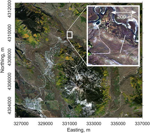
FIGURE 1. Aerial view (WordView-2 RGB composition) of the site located in the upper East River watershed near Crested Butte, CO. The investigation included a 60 m wide corridor along a 160 m long ERT transect (white line) that covers a hillslope, its toe and a small portion of the adjacent floodplain.
The geology in the region is mainly composed of sediments with various degree of metamorphism, and includes the Cretaceous Mancos Shale formation which is about 1,500 m thick (Hamilton, 1972; Uhlemann et al., 2022). In some places, outside the investigated site, the sediment layers have been intruded by igneous rocks. The soil present in the region includes shale rock land, Tilton sandy loam, Teoculli loam, Cryaquolls and Histosols (https://websoilsurvey.sc.egov.usda.gov). The hillslope soil textures are generally loam to silt loam, with increasing fraction of fines toward the bottom of the hillslope and silty clay and silty clay loam in the floodplain (Tokunaga et al., 2019; Yan et al., 2021). Soil thickness measurements obtained by identifying the contact layer between soil and weathered bedrock vary between 0.15 and 1.5 m, with a mean value of 0.76 m. The soil thickness shows an increasing trend toward the bottom of the hillslope with largest values in topographic lows and in the floodplain (Yan et al., 2021).
Meteorological forcing at the site involves snowpack accumulation from November through mid-April, with snowmelt occurring in the spring season (March-June) and peak of snow-water-equivalent in mid-April. Meteorological data obtained from the Butte Snow Telemetry (SNOTEL) station located 2 km from the site and 350 m higher in elevation (https://wcc.sc.egov.usda.gov/nwcc/site?sitenum=380) indicate a mean daily air temperatures that ranges from −8.3°C in December to 11°C in June. Annual precipitation for 30-year period of record at Butte SNOTEL station is 670 ± 120 mm/year with snow accounting for 66% ± 12% annual precipitation (Carroll et al., 2018). This study covered the water year (WY) 2017 (time interval from 1 October 2016 to 30 September 2017) and WY2018 (time interval from 1 October 2017 to 30 September 2018). WY2017 was a high water year with a deep snowpack and late snowmelt, whereas WY2018 was a low water year, with low snowpack and early snowmelt. The peak Snow Water Equivalent (SWE) in WY2017 is 2.1 times larger than in WY2018. Considering the 1991–2020 record for SWE at the Butte SNOTEL station, WY2017 is close to the 70th percentile with regard to the first bare-ground date and 90th percentile with regard to peak SWE. WY2018 is close to the 10th percentile with regard to the fist bare-ground date and peak SWE. The Community Land Model (CLM) (Oleson et al., 2013) was used to delineate spatiotemporal variations in evapotranspiration (ET) with 900 m resolution across the East River Watershed (Tran et al., 2019). Application of this analysis to the hillslope field site for WY2017 and WY2018 yielded ET of 310 and 288 mm, respectively (Tokunaga et al., 2019). It also confirmed that ET rises rapidly during snowmelt and that snowmelt is the major source of water for the system, including for plant growth and potential recharge to groundwater.
Time-lapse imagery was collected 4 times in 2017 and 4 times in 2018 using a 3DR Solo UAV platform. In both years, the aerial surveys involved the collection of RGB imagery using a Sony 5,100 digital camera. In addition, multi-spectral reflectance imagery was collected with a Micasense Rededge camera in 2017. The UAV surveys were performed across a 300 x 500 m2 area encompassing the studied hillslope transect. About 50 small PVC targets were deployed and used as Ground Control Points (GCPs) for accurate georeferencing of the UAV-based imagery. The GCPs centers were measured prior to each UAV flights with a Real Time Kinematic (RTK)-GPS. The multi-spectral reflectance data were calibrated using a diffusive reflectance target provided by Micasense. All georeferenced orthomosaics and digital surface model (DSM) were reconstructed using AgiSoft reconstruction software using structure-from-motion-based reconstruction techniques (e.g., James and Robson, 2012).
The resulting georeferenced orthomosaics and DSMs, with a resolution ranging between 2 and 10 cm, were all interpolated to 10 cm pixel resolution for comparison purposes. Comparison of the orthomosaics and DSM at various times with reference GCPs across the surveyed area showed that the uncertainty in x, y, z was in the order of 10 cm. We inferred GCC from the RGB imagery and NDVI from the Rededge multi-spectral imagery. NDVI is defined as (NIR-R)/(NIR + R) and the GCC is defined as [G/(R + G + B)], where B, G, R and NIR represent the blue, green, red, and near-infrared channel, respectively (e.g., Sonnentag et al., 2012). While the general quality of the dataset can be considered as high, we found that the blue band from the Rededge camera was not always reliable and thus GCC was calculated from the RGB dataset only. In addition, the DSMs inferred from the RGB camera dataset were used to estimate changes in plant height over time by subtracting the LiDAR dataset from the DSMs.
Airborne LiDAR data were acquired over the study area on 10 August 2015, using a Riegl Q1560 dual-channel LiDAR system and provided a point density with more than 8 pulses/m2 that was used to create a digital terrain model (DTM), representing the first bare-ground elevation, at a spatial resolution of 0.5 m (Falco et al., 2019a). The DTM was compared with RTK GPS measurements (positioning accuracy within few centimeters) in a vegetated region within the hillslope; the root-mean-square-error of the DEMs was less than 0.15 m. The DTM was used to infer topographic metrics including slope and topographic wetness index (TWI).
A map of the vegetation type was obtained by using the Lidar data, an optical satellite image acquired by the WorldView-2 on 24 September 2015, and ground-based spectral measurements and identification of plant communities (Falco et al., 2019a). Vegetation classes were determined based on distinct spectral or structural signatures as well as their importance for ecosystem functioning.
Landsat 8 imagery (Irons et al., 2012) during the growing season of WY2017 and WY2018 was used to obtain surface reflectance and calculate the NDVI and GCC across a 200 m side region encompassing the transect. Only the datasets without cloud cover were considered. Due to the Landsat spatial resolution of 30 m, this dataset is only used to evaluate the temporal trends in WY2017 and WY2018 and compare them to the trends observed in the UAV-based imagery.
Continuous measurement of soil moisture and temperature were obtained using 5 TE soil moisture sensors (Meter Inc.) at 0.1 and 0.5 m depth at three locations along the transect. The three locations referred further as SM1, SM2 and SM3 are located at 66 m, 103 m and 123 m along the transect, respectively. SM1, SM2 and SM3 are located on the hillslope, at the hillslope toe and on a very small ridge separating the hillslope toe and the floodplain, respectively. SM2 is located in a patch of veratrum, while the two other locations are located in area with predominantly forb and some sparse sagebrush. The time-series of soil moisture and temperature cover most of the 2016–2019 window but data are missing for several time intervals due to logger failure or animal disturbance (<5% data missing). The first bare-ground date in WY2017 and WY2018 was defined when air temperature diurnal fluctuation led to a temperature fluctuation of a few degrees at 0.1 m depth. For the comparison with the ERT data at a similar spatial resolution, the soil moisture data at 0.1 and 0.5 m depth were vertically averaged at each of the three locations. The porosity is defined here as the soil moisture value at saturation during the WY2017 snowmelt period.
Electrical resistivity tomography (ERT) data were autonomously acquired over the transect using a 1.25 m electrode spacing and a dipole-dipole array configuration. The data were collected using a MPT DAS-1 electrical impedance tomography system linked to a field computer, both powered with a solar panel installation. Data were collected daily from October 2016 to November 2017. Power limitation or failure, and animal damage led to several gaps in data with about 20% and 80% data missing in WY2017 and WY2018, respectively.
The acquired resistance data were used to reconstruct a 2D model of depth-discrete soil electrical conductivity (or resistivity) along the transect using a smoothness-constraint inversion code named boundless electrical resistivity tomography (BERT) (Rücker et al., 2006; Rücker et al., 2006). Low-quality measurements were removed prior to the inversion, including signals associated with measured potentials less than 1 mV. Reciprocal measurements acquired a few times during the growing season were used to remove noisy data linked to a few electrodes with high-contact resistance during dry conditions. The inversion of each data set was done with the same mesh and parameterization and independently. An anisotropic ratio of two between horizontal and vertical regularization was used. The obtained tomography shows a smoothed image of the spatial distribution of soil bulk conductivity with a vertical resolution of roughly a third to a half of the electrode spacing near the surface, which corresponds to about 50 cm.
The soil electrical conductivity is influenced by subsurface characteristics such as soil moisture, porosity, fluid electrical conductivity, clay content, and soil temperature (e.g., Archie, 1945; Revil et al., 1998; Friedman, 2005). Depending on the environment, the spatial variability in electrical conductivity can be predominantly driven by one of the above characteristics, including clay content (e.g., Triantafilis and Lesch, 2005; Falco et al., 2021), salinity (e.g., Corwin and Lesch, 2005) or water content (e.g., Dafflon et al., 2017; Thayer et al., 2018) or a combination of them (e.g., Dafflon et al., 2013; Uhlemann et al., 2017). In this study, we consider only the near-surface soil electrical conductivity as averaged from 0 to 50 cm depth, which is an important zone for plant-soil interactions. It is to note that in this study the ERT data are not used to estimate the soil thickness because of the large electrode spacing relative to the soil thickness measured at the site (Yan et al., 2021) and the limited contrast in electrical conductivity between the soil and the weathered shale bedrock. Temperature correction is critical to analyze near-surface electrical conductivity over time given that temperature variation between first bare-ground date and the summer time can be as high as 16°C at 50 cm depth, which implies a 30% change in electrical conductivity due to temperature at this depth. To remove the temperature effect on soil electrical conductivity, we applied a temperature correction of 1.9% increase in fluid electrical conductivity per degree Celsius (Hayley et al., 2007) and infer electrical conductivity at a reference temperature of 20°C. The correction was done using the soil temperature data at 50 cm depth at the three locations equipped with soil moisture sensors. The correction was specific to each location for the bivariate analysis between soil moisture and soil electrical conductivity data but we used the average temperature between the three locations for correction of the entire electrical conductivity transects.
The soil moisture spatiotemporal distribution along the hillslope transect is estimated with four approaches that rely on various datasets and thus can provide different spatial coverage. These approaches, which build on the dynamics observed from the soil moisture sensors and the ERT, include 1) a single (i.e., for space and time) logarithmic linear regression between soil moisture measurements from the point-scale sensor and soil electrical conductivity from the ERT data, 2) the use of soil moisture data under saturated conditions to estimate porosity and soil electrical conductivity to estimate the temporal variability in water saturation, 3) the use of a logarithmic linear regression between soil moisture and soil electrical conductivity during saturated conditions to estimate porosity, coupled with the use of a spatially averaged variation in soil moisture (between minimum and maximum soil moisture observed at each of the three sites), and 4) the use of a simple linear regression between soil moisture under saturated conditions and GCC acquired close to the peak of the growing season–based on the assumption that peak GCC is a direct response to water content during snowmelt–to predict porosity and the use of the spatially averaged variation in soil moisture across the three sites to estimate soil moisture over space and time across the UAV-acquired GCC domain.
The second approach differs from the other approaches in that the temperature corrected soil electrical conductivity is related to soil moisture (
where ϕ, S, σw,T20, n and m are the porosity, the saturation (
where n falls within the range of 1.0–2.7 typically (Ulrich and Slater, 2004) and is here set to 2. In this study, we use Eq. 2 to evaluate how well the saturation component inferred from the temporal changes in soil electrical conductivity could be used to estimate soil moisture when combined with porosity inferred from soil moisture measurements at saturation.
We first explore the spatial variability in UAV-based estimate of GCC, NDVI and plant height and the soil electrical conductivity across the transect and how these characteristics are linked to topographic metrics and plant type at the peak of the growing season in WY2017. The peak of the growing season is defined here as the time when the spatially averaged value of GCC is the highest, though we recognize that different plant types may reach their peak in vigor and density at slightly different times.
We observe strong co-variability between above-, on- and below-ground characteristics at the peak of the growing season on 8 July 2017 (Figures 2, 3), with the strongest correlation between independently-measured properties including soil electrical conductivity, GCC, plant height, and slope. In particular, the Pearson correlation coefficients (r) are high for the relations between soil electrical conductivity and GCC (r = 0.74), plant height (r = 0.61) and slope (r = 0.58), and between plant height and slope (r = 0.63) and GCC (r = 0.61). Relationship involving NDVI and TWI are weaker (r < 0.58). These results are consistent with the study of Falco et al. (2019a), that evaluated the co-variability of plant types, slope and a single time ERT dataset acquired in September 2016.
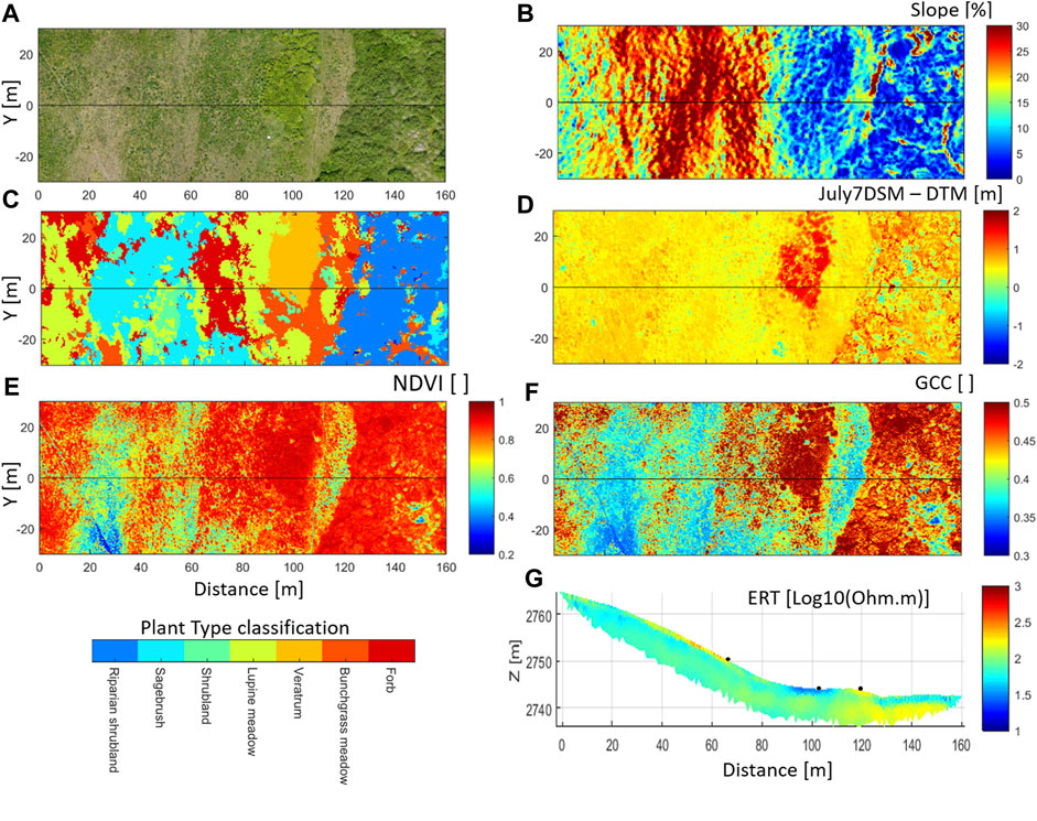
FIGURE 2. (A–F) Topographic and vegetation characteristics on 8 July 2017 along a 160 x 60 m wide corridor with a central ERT transect location (indicated with the black horizontal line); (A) RGB orthomosaic, (B) slope derived from LiDAR DTM, (C) plant type classification (Falco et al., 2019a), (D) plant height inferred from subtracting the LiDAR DTM from the DSM, and UAV-inferred (E) NDVI and (F) GCC. (G) ERT with black dots indicating the soil moisture sensors locations at 66 m, 103 m and 120 m along the ERT transect, which ends 60 m before crossing the upper East River.
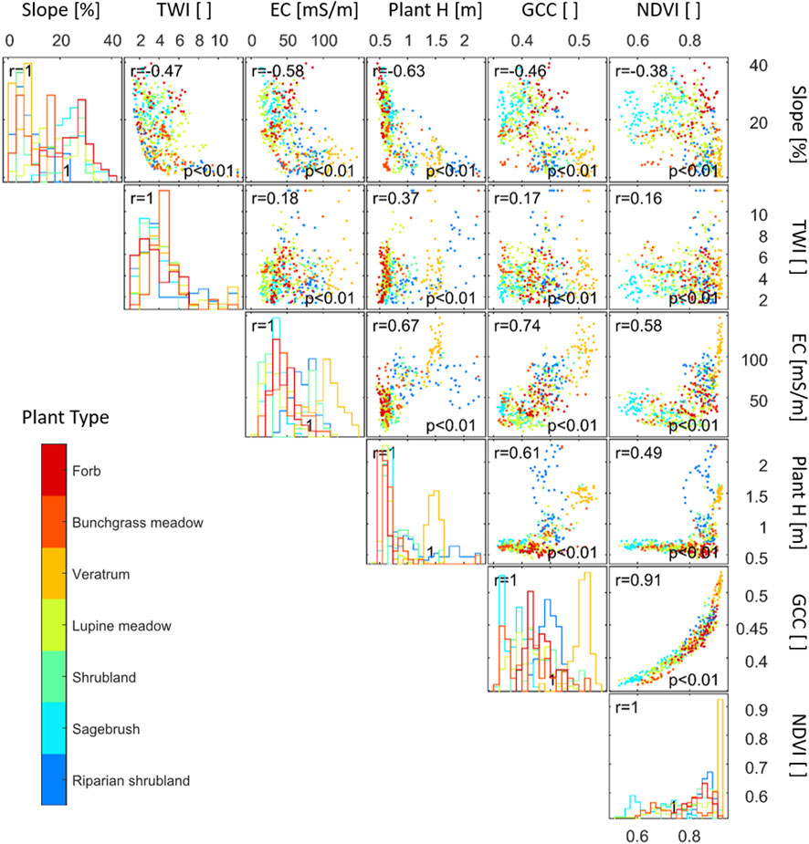
FIGURE 3. Cross correlation between and relative frequency distribution of various characteristics including slope, topographic wetness index (TWI), soil electrical conductivity (EC), plant height, GCC and NDVI on 8 July 2017. The various colors refer to the various plant type. The correlation coefficients (r) and their statistical significance (p values) are shown in each cross-correlation plot on the top left and bottom right corners, respectively.
Locations with similar vegetation types are strongly clustered as a function of surface and soil characteristics that are expected to be adequate in fulfilling vegetation specific physiological demands (Figure 3). End members include sagebrush (low GCC) at sites with low electrical conductivity and high slope, and veratrum and riparian shrubs (high GCC) with high electrical conductivity and low slope. Plants such as veratrum and riparian shrubland consistently occupy depressions or flat areas that are close to level and have high soil moisture, while plants such as sagebrush grow along ridges or moderate steep areas with limited soil moisture. Overall, the results confirm that hillslope vegetation selects, adapts to, exploits, and thus expresses the integrated water-energy-nutrients environment (Fan et al., 2019).
Both NDVI and GCC capture spatial variability in plant vigor and density, although quite differently due to their different sensitivity (Figure 3). The exponential relationship between GCC and NDVI is observed on 8 July 2017, as well as at other times during the growing season (Supplementary Figure S1). Landsat data show a similar relationship between GCC and NDVI, confirming their different sensitivity to vegetation vigor and density. GCC is relatively insensitive to subtle changes in low plant vigor and density (e.g., at the beginning of the season) compared to NDVI, while at later times, NDVI saturates, while GCC still captures a large range of high GCC values. This different sensitivity implies that NDVI is better correlated with the soil electrical conductivity at the beginning of the growth season while at later time (with high NDVI values) this correlation diminishes. Inversely, GCC becomes correlated with soil electrical conductivity later in the growing season, but the relationship gets increasingly strong over time. Thus, capturing a large range of values in plant vigor and density requires a different timing for NDVI than for GCC, while capturing the full range of spatial variability using NDVI can only be achieved during a relatively short time-window before the peak of the growing season. Due to the above observations and the fact that NDVI is more challenging to infer than GCC, we concentrate on the use of GCC in the rest of this study.
The main variations in soil moisture and electrical conductivity in the top 0.5 m of soil in WY2017 and WY2018 result from snow melt events occurring from March to May, increasing soil moisture up to saturation. This period is followed by a gradual decrease in soil moisture. Summer rain events create only small and intermittent increases in soil moisture, with similar amounts in WY2017 and WY2018 (Figure 4).
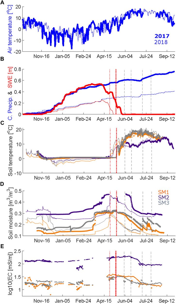
FIGURE 4. Time-series of atmospheric, snow and soil variables for WY2017 (thick lines) and WY2018 (thin lines); (A) air temperature and (B) cumulative precipitation and snow water equivalent from Butte SNOTEL station located 2 km from the site and 350 m higher in elevation; (C) soil temperature at 10 cm depth, (D) soil moisture averaged between 10 and 50 cm depth, and (E) temperature corrected soil electrical conductivity (EC) in the top 50 cm of soil at 66 m (SM1, orange), 103 m (SM2, purple) and 120 m (SM3, grey) along the ERT transect. Soil electrical conductivity has been acquired fairly continuously in WY2017 (small dots) but very sparsely in WY2018 (large dots). The first bare-ground dates for WY2017 (thick vertical red line, 13 May) and WY2018 (thin vertical red line, 26 April) have been inferred by the onset of diurnal fluctuations in the soil temperature at 10 cm depth. The vertical grey lines indicate dates when UAV data were acquired in WY2017, and approximately in WY2018. It can be noted that the high and relatively constant soil moisture values observed during the spring of WY2017 correspond to soil water saturated conditions and a groundwater table close to the ground surface.
The major difference between the WY2017 and WY2018 soil hydrological dynamics is in the timing of the infiltration event leading to soil saturation, and the time-interval until the later decrease in soil moisture after the first bare-ground date (Figure 4). In WY2017 an initial increase in soil moisture is observed as early as January 21, while soil saturation was reached at the three monitored locations between March 20 and April 13 and lasted until early-to mid-June. In WY2018, soil at the same locations remained saturated for a few days only, starting on April 25. Earlier increase in soil moisture occurred on March 16, while the soil between 0 and 50 cm depth was partially frozen before that date. The first bare-ground date at the site in WY2017 and WY2018 was May 13 and April 26, respectively. After the snow melt, the first decrease in soil moisture occurred between May 27 and June 13 in WY2017, and between April 28 and May 3 in WY2018. In other words, WY2018, in comparison with WY2017, is characterized by a 50 days later first increase in soil moisture during the winter, a 12–35 days delay in reaching soil water saturation, a 17 days earlier first bare-ground date, and a 24–48 days earlier decrease in soil moisture after the end of snowmelt. Indeed, the decay in soil moisture in WY2018 occurred only 1 day after the first bare-ground date, while this event occurred between 14 and 30 days after the first bare-ground date in WY2017. It clearly shows the combined effect of WY2018’s thinner snowpack, frozen ground and earlier first bare-ground date on the reduced amount of water infiltration and time the soil was water saturated. Also, the short period of time involving soil water saturated conditions in WY2018 (∼3 days) and its end right after the first bare-ground date indicates that the high moisture content was primarily driven by the snowmelt induced vertical percolation at these locations. On the contrary, the much longer period of time with saturated conditions in WY2017 (∼73 days) results not only from more infiltration at these locations but also a shallow groundwater table depth. The presence of the groundwater table near the surface was confirmed by the earlier increase in soil moisture data at 0.5 m than at 0.3 m depth in WY2017 (not shown), as well as by groundwater level data from nearby wells at the top and bottom of the hillslope indicating that the water table remained remarkably close to the soil surface and that groundwater table rised in the top 0.5 m of soil in WY2017 while being deeper than 1 m in WY2018 (Tokunaga et al., 2019).
The highest values in soil moisture, at all times, are observed at the hillslope toe, primarily covered with veratrum (Figure 2). The timing in soil moisture variations varies along the transect with earliest increase in soil moisture occurring at the hillslope toe, soil saturation was reached slightly later at the hillslope toe than on the hillslope and topographic high, and water saturated conditions remaining the longest at the hillslope toe. Despite the above differences, the timing and the magnitude of increase and decrease in soil moisture at the three locations show similarities when compared to the inter-annual variability in soil moisture dynamic. A main difference between the three locations is their maximum soil moisture (i.e., porosity) and the minimum soil moisture (under unfrozen conditions) (Figure 4). We obtain porosity equal to 0.31, 0.47 and 0.33 m3/m3, minimum soil moisture equal to 0.15, 0.29 and 0.17 m3/m3 and thus range in soil moisture variation equal to 0.16, 0.18 and 0.16 m3/m3 for SM1, SM2 and SM3, respectively. Thus, the soil moisture data at the three sites are linked to very different porosity and minimum soil moisture, while they show relatively similar range in soil moisture variation. It is to note that we do not intend to assess a potential link between the estimated minimum soil moisture and a residual soil moisture or the wilting point, since it would require additional measurements. Also, quantifying the individual controls on the spatiotemporal variability in soil moisture along the hillslope, such as differences in landscape position, soil texture and hydraulic properties, and evapotranspiration, is challenging and beyond the scope of this study.
The soil electrical conductivity measurements suggest that even though the mean value changed over time, the spatial relative variability in electrical conductivity along the transect remained fairly similar over time. First, the electrical conductivity collocated with the soil moisture data shows similar ranking of more conductive to less conductive locations related to wetter to drier sites (Figure 4). Second, the temporal correlation between various snapshots is generally strong, as shown in Figure 5, where the temperature-corrected soil electrical conductivity for the top 50 cm along the entire transect during WY2017 and WY2018 is presented and used to evaluate the correlation coefficient between a reference snapshot and every other one. Indeed, outside the WY2018 winter when the soil was partly frozen, the correlation coefficient remained higher than 0.8 at all times. It indicates that while the conductivity for the entire domain fluctuates with regard to absolute value, the spatial variability remains relatively constant over time. It is consistent with the observation that all locations synchronously become wetter or drier and that the ranking in wet to dry locations does not change much over time. However, it is to note that this dynamic is field site specific and can be modulated by a complex combination of various soil characteristics and processes that impact the spatiotemporal variability in electrical conductivity. Overall, the observed temporal correlation is consistent with a study using a similar monitoring approach in an Arctic environment (Dafflon et al., 2017) that found that the temporal correlation coefficients in ERT transect data exceeded 0.8 over the entire growing season. The observation of a spatial pattern in wetness persisting over time was also found in other studies. For example, the study of Lowry et al. (2011) in a mountain meadow in the Tuolumne River basin, California revealed temporally persistent spatial pattern in soil wetness driven by the groundwater table dynamics, and co-variability of this moisture pattern and vegetation composition.
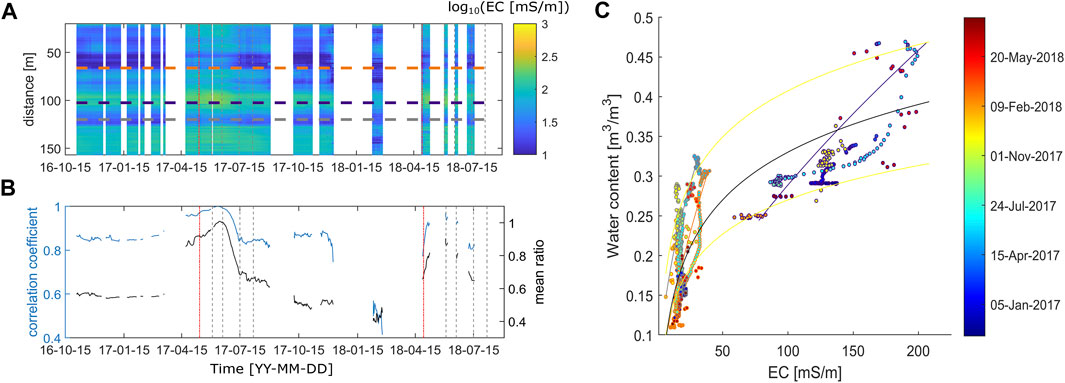
FIGURE 5. (A) Soil electrical conductivity in the top 50 cm over time and (B) correlation coefficient and mean ratio between 10 June and all other times. Horizontal orange, blue and grey lines in (A) indicate SM1, SM2 and SM3 location, respectively. Vertical red and grey lines indicate the first bare-ground dates and the UAV survey dates, respectively. (C) Bivariate relationship between collocated soil moisture and electrical conductivity (EC) data. The logarithmic relationship (black line), which would correspond to a linear relationship between the decimal logarithm of soil electrical conductivity and soil moisture, provides a RMSE of 0.0495 and a ME of 0.0435 m3/m3. The location specific relationship (Eq. 2) for SM1 (orange), SM2 (purple) and SM3 (grey) provide a RMSE of 0.037, 0.039 and 0.039 m3/m3, respectively. The two yellow lines represent a logarithmic function fitted to the lowest and highest values in soil moisture and electrical conductivity.
To evaluate the soil moisture variability along the transect from a few soil moisture sensors and the ERT dataset, we tested three different approaches (described in Section 2.2.5) The first approach, which involves a single logarithmic relationship between both variables provides a Root Means Square Error (RMSE) of 0.0495 m3/m3 and a Mean absolute Error (ME) of 0.0435 m3/m3 (Figure 5). The second approach, which makes use of location-specific relationship using Eq. 2, with soil porosity obtained from the soil moisture data under saturated conditions, enables more reliable estimation of soil moisture with a RMSE of 0.037, 0.039 and 0.039 m3/m3, and a ME of 0.032, 0.033 and 0.033 m3/m3 for SM1, SM2 and SM3, respectively (Figure 5). However, the use of the second approach to estimate soil moisture dynamics at more locations than monitored with point-scale sensors is not very practical, as it requires numerous discrete measurements of porosity, for example, by measuring soil moisture under water saturated conditions along the entire ERT transect right after the first-bare ground date using a portable time-domain reflectometer. The third approach consists in fitting a logarithmic relationship between the maximum soil moisture and soil electrical conductivity values to estimate porosity along the transect at the time of complete soil saturation and the spatially averaged variations in soil moisture across the three sites to estimate soil moisture over space and time along the entire transect (Figure 6). Our decision of averaging the variation in soil moisture is based on the presence of a relatively similar range of variation in soil moisture at the three sites, as well as similarities in how soil moisture varies over time (Section 3.3). The obtained RMSE and ME for soil moisture estimated using this approach at the three moisture sensor locations are equal to 0.029, 0.032, 0.036 and 0.028, 0.027, 0.032 m3/m3, respectively. The overall RMSE and ME across all three locations are equal 0.033 and 0.029 m3/m3, respectively, which is lower than using a single logarithmic relationship or Eq. 2. The third approach is, therefore, used to evaluate the co-variability between soil moisture and vegetation dynamic along the entire transect. It is to note that the above approaches show RMSEs relatively similar to other studies involving soil moisture and electrical conductivity at the field scale (Cardenas and Kanarek, 2014; Thayer et al., 2018). The RMSE for water content regression in Thayer et al. (2018) and Cardenas and Kanarek. (2014), is 0.024 m3/m3 and 0.042 m3/m3, respectively. The results of this study confirm the range of uncertainty present in estimating soil moisture from electrical conductivity data along heterogeneous transects, and provide with other studies some baseline for comparing different strategies. Further, the above results confirm the need to develop integrated approaches that capture both the soil porosity and the variability in soil saturation.
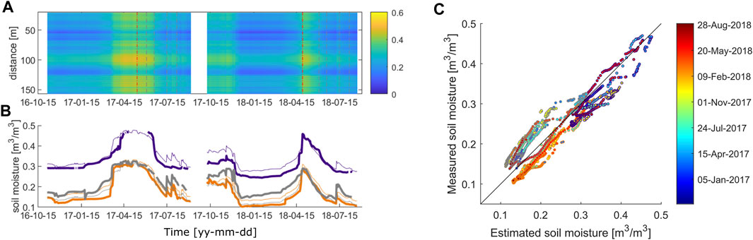
FIGURE 6. (A) Spatiotemporal reconstruction of soil moisture [m3/m3] distribution using spatially averaged variation in soil moisture and a simple linear regression between porosity and maximum electrical conductivity. (B) measured (thick line) and estimated (thin line) soil moisture over time and (C) versus each other. RMSE at SM1 (orange), SM2 (purple) and SM3 (grey) are equal to 0.029, 0.032 and 0.036 m3/m3, respectively, and the overall RMS is equal 0.033 m3/m3.
To investigate the timing in interactions between soil and plant as a function of position in a hillslope to floodplain domain, we evaluate the spatial and temporal dynamics in the relationship between several soil and plant variables from first bare-ground date to senescence in WY2017 and WY2018. Figure 7 shows the dynamic in soil and vegetation variables in WY2017 and WY2018, as well as the bivariate relationship between soil electrical conductivity and GCC at the time of UAV-based surveys. Figure 8 shows the relationship between the soil moisture estimated using the third approach described in Section 2.2.5 (Figure 6) and GCC as a function of plant type for WY2017 and WY2018.
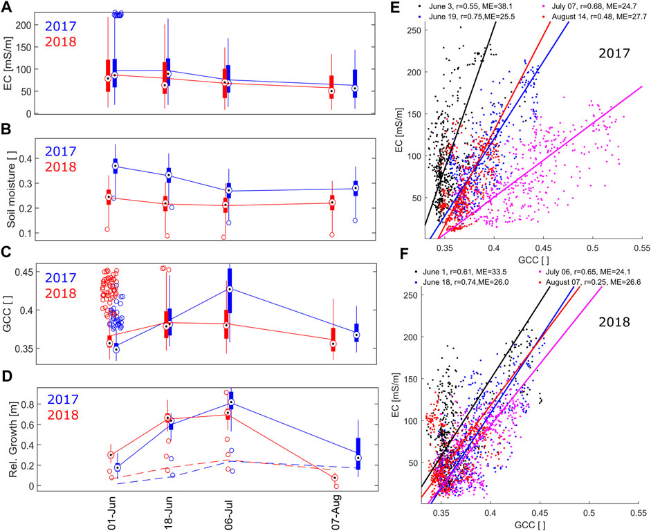
FIGURE 7. Dynamics in soil and vegetation variables in WY2017 and WY2018. (A) soil electrical conductivity, (B) estimated soil moisture (Figure 6) along the ERT transect, and UAV-inferred (C) GCC and (D) relative growth in veratrum (solid line) and average trend when considering all plant types (dashed line) along the studied transect. Each colored rectangle indicates the lower to upper quartile range with the median value shown with a black dot. Each vertical line represents the whisker that reaches the value that is the furthest from the median while still being inside a distance of 1.5 times the interquartile range from the lower or upper quartile. Values outside the whisker are shown with circles. (E–F) Bivariate analysis between GCC and soil EC on (E) 3 June, 19 June, 7 July and 14 August 2017, and (F) 1 June, 18 June, 6 July and 07 August 2018. In (E–F) the correlation coefficient (r) and the Mean absolute Error (ME) (mS/m) of the fitted linear relationships are provided.
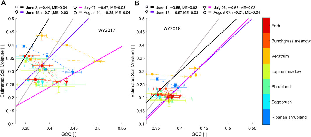
FIGURE 8. Bivariate analysis between GCC and estimated soil moisture (Figure 6) in (A) WY2017 and (B) in WY2018. Dot colors and shapes indicate plant type and time of acquisition, respectively. The color of the regression line represents the time of acquisition. The dashed lines in (A–B) highlight the temporal co-dynamic in GCC and estimated soil moisture for the various plant types from 3 June to 14 August.
The bivariate analysis between vegetation indices with shallow soil electrical conductivity at different times in WY2017 and WY2018 shows variable relationships and strength during the year, with the strongest amplitude in GCC in high water year (WY2017) (Figure 7). The beginning of the growing season is marked by low values of GCC and a large range of soil electrical conductivity. As plants grow, the range of GCC values becomes larger, while electrical conductivity values slowly decrease. The highest GCC values are observed on 8 July 2017. The linear relationship between GCC and electrical conductivity in WY2017 is the strongest on 8 July 2017 (ME=24.7 mS/m), followed by June 19 (ME=25.5 mS/m), and June 3 (ME=38.1 mS/m). The relationship is strongly driven by the presence of wet locations where greening is strong, while dry locations having low electrical resistivity are less variable over time. As a result, the slope and intercept of the relationship vary over time. These results indicate that the greenness values alone cannot be linked to electrical conductivity with a unique relationship remaining constant over time.
Various plant types show distinct greening trends and maximums that are also linked to the distinct distribution of soil electrical conductivity or moisture at the first bare-ground date and later time points. Though a positive correlation between soil moisture and GCC exists at a single point in time, they are negatively correlated when looking at a specific plant type (e.g., veratrum) over time (Figure 8). For several plant types, the soil moisture decreases continuously after the first bare-ground date while GCC increases. The use of NDVI indicates relatively similar trends, while clearly showing its tendency to saturate at high vegetation biomass (Supplementary Figure S2). Plant types linked with high electrical conductivity and soil moisture at the beginning of the growing season, such as veratrum and shrubs in the riparian zone, show the strongest seasonal increase in GCC. When observing the relationship across space vs. time, the opposite trend is noted owing to the time lag between changes in soil moisture and plant states. It can be noted that the GCC distribution obtained from a UAV survey along the transect on the first bare-ground date 26 April 2018 (data not shown), shows a 95% confidence interval of 0.331 ± 0.008, which indicates that all plants have a very similar GCC before the growing season and thus that GCC at later time is primarily resulting from the seasonal plant growth.
While soil moisture and electrical conductivity in both years reach the same value during the snowmelt period (Figure 4), WY2018 is marked by an early bare-ground date and a very short duration of water saturated conditions in the soil. As a consequence, GCC values in WY2018 only exceed those observed in WY2017 in early June (Figures 7, 8). Though delayed by a later first bare-ground date, GCC in WY2017 rapidly exceeds values observed during the duration of the WY2018 growing season. The veratrum plant heights confirm the higher productivity in WY2017 by showing a temporal pattern similar to GCC (Figure 7). Further, while in WY2018 several rain events occurred in late June and early July, they do not counter-balance the described trend. It is to note that the vegetation and soil dynamics and their interactions with summer rain in this lower montane environment at an elevation of about 2,800 m may differ from those at higher elevations and/or in different plant community (Carroll et al., 2019).
Overall, the above results are consistent with the co-variability observed between vegetation indices and soil moisture patterns (e.g., Devadoss et al., 2020). In particular, the fact that the various plant types show relatively similar slopes between increase in GCC and decrease in soil moisture (Figure 8) indicates the strong impact of the initial condition in soil moisture on the GCC value at the peak of the growing season. It demonstrates that the vegetation indices at the peak of the growing season–or at their maximum for each location–provides a good indicator of inter-annual variations in hydrological status, confirming the link between Landsat-derived annual peak NDVI and June Palmer Drought Severity Index (PDSI) (Chen et al., 2021) and the first bare-ground date observed across the East River watershed (Wainwright et al., 2020). Further, the above results indicate that plant types linked to high soil moisture values, such as veratrum and shrubs in the riparian zone, lead to particularly strong increase in GCC over the season. Besides being valuable indicators for monitoring plant seasonal dynamic due to their large dynamical range in GCC versus data uncertainty, capturing their spatial distribution and dynamics is relevant to reduce the uncertainty in carbon fluxes and storage in such environment. Indeed, studies have shown that locations where water converges and/or is retained and where soil accumulates (Yan et al., 2021), as often in montane meadow in low-gradient valley or hillslope toe, represent a strong source of uncertainty in the estimation of carbon storage and emission (e.g., Reed et al., 2021).
The strong link between GCC at the peak of the growing season and the soil moisture distribution allows for the possibility to use plant greenness to infer the spatial variability in soil moisture. We use the relationship between the GCC on June 19 and maximum soil moisture measured during snowmelt to estimate the porosity over space, and we use the spatially averaged variation in soil moisture across the three sites to estimate soil moisture over space and time along the hillslope (Figures 9, 10). Besides the use of GCC, this approach is similar to the previous approach where soil electrical conductivity was used. The obtained RMSE and ME for all three locations are 0.023, 0.026, 0.035 m3/m3 and 0.021, 0.021, 0.031 m3/m3, respectively. The overall RMSE and ME across all three locations are 0.029 and 0.025 m3/m3, respectively, which is lower than using relationship involving the electrical conductivity (Section 2.2.5).
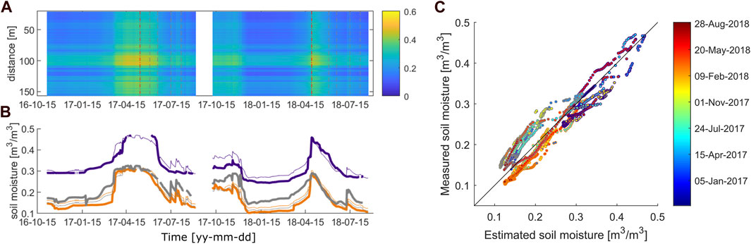
FIGURE 9. (A) Spatiotemporal reconstruction of soil moisture [m3/m3] estimated using the spatially averaged variation in soil moisture and a simple linear regression between porosity and GCC close to the peak of the growing season (17 June). (B) Time series of measured (thick line) and calculated (thin line) soil moisture and (C) measured vs. calculated soil moisture for different dates. RMSE at SM1 (orange), SM2 (purple) and SM3 (grey) are equal to 0.023, 0.026 and 0.035 m3/m3, respectively, and the total RMS is equal to 0.029 m3/m3.
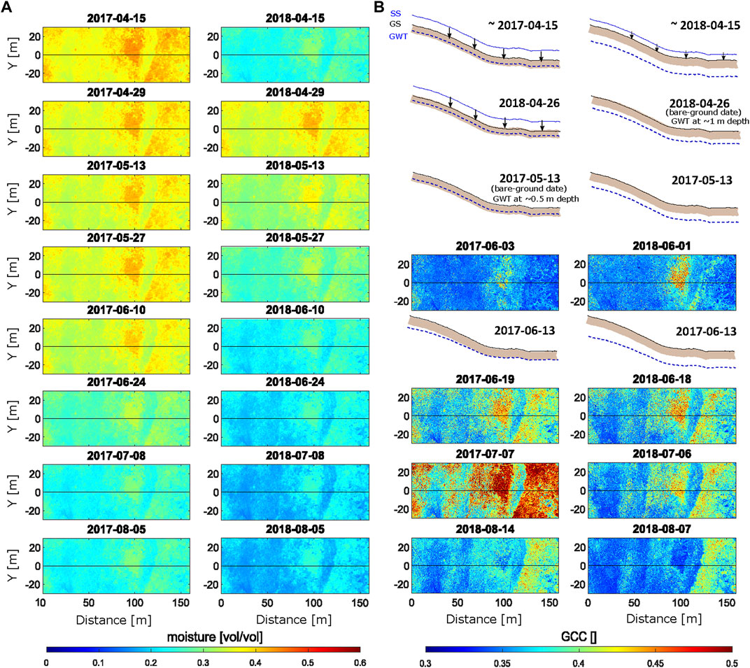
FIGURE 10. Seasonal dynamics in soil moisture and vegetation. (A) Estimated soil moisture in the top 0.5 m of soil across the hillslope (shown in Figure 2) in WY2017 and WY2018 at 14- and 28-day interval from 15 April to 8 July and 8 July to 5 August, respectively. (B) UAV-inferred vegetation GCC in WY2017 and WY2018 and schematics illustrating major hydrological processes. The Groundwater Table (GWT) depth, snow surface (SS), ground surface (GS) and top 0.5 m of soil (brown) are represented to illustrate the major difference between WY2017 and WY2018, specifically the soil remaining wet much longer in WY2017 due to a larger amount of snow, a later first bare-ground date, and a GWT maintained near the ground surface for a long period of time due to significant local and upslope snowmelt events.
Besides providing lower RMSE than the other approaches tested in this study, the approach using GCC and soil moisture sensors to estimate the soil moisture spatiotemporal distribution has the advantage of being more scalable as vegetation indices can be collected using UAV or satellite imagery. Still, this approach is only applicable at local scale because the estimation of soil moisture in this study relies on the observation that the temporal variations in soil moisture was relatively similar at various locations along the hillslope (when compared to inter-annual variability). The reliability of this approach is expected to decrease strongly with increasing spatial coverage, due to increasing heterogeneity in snowpack dynamic, topographic position, and soil physical and hydraulic properties. Although several studies have developed approaches for large-scale, high-resolution estimation of soil moisture using vegetation indices–primarily for agricultural purpose–, accounting for the time lag between changes in soil moisture and corresponding changes in the vegetation indices is recognized as challenging (Zhang and Zhou, 2016). An approach to reduce error in soil moisture estimation is to involve models or data that account for the direct effect of water infiltration events on soil moisture, which is obviously easier to achieve in rain-than snow-impacted environment (e.g., Acharya et al., 2022). Our results indicate that the identified link between vegetation indices and soil moisture in the studied snow-dominated environment is promising to constrain the reconstruction of the spatiotemporal distribution of soil moisture, although soil moisture and/or snowmelt rate datasets are essential. Currently, extending the approach used in this study beyond a single hillslope would require a strategic placement of sensors to capture the range of soil moisture dynamics. Finally, while the UAV provided unparallel spatial resolution in plant greenness in this study, the increasing emergence of satellite products having meter scale resolution is quickly becoming a preferable alternative to reduce the cost of acquisition and processing time.
Drought conditions are likely to intensify in the future as climate models predict both earlier snowmelt and less snowfall throughout western North America (e.g., Diffenbaugh et al., 2013; Fyfe et al., 2017). Results of this study confirm that in a lower montane environment an earlier bare-ground date, which is often linked to low snowpack year, is an indicator of later plant drought conditions which can constitute a threat to plant viability (e.g., Iler et al., 2019). An increase in productivity due to longer growing season would only occur in systems that are not water limited (Ernakovich et al., 2014).
The inter-annual difference in soil moisture dynamics and associated plant seasonal dynamics confirm that in the studied lower montane environment, the vegetation productivity in a heavy snow year (WY2017) benefits from both greater water infiltration as well as a shallower groundwater table depth (Figures 4, 10). Tokunaga et al. (2019) documented that infiltration along this hillslope does not reach the groundwater table for the majority of time, except for the snowmelt period. Our study shows that a groundwater table rising close to the ground surface due to large local and upslope snowmelt water infiltration can maintain a saturated near-surface soil for several weeks. Its decline controls the onset of the soil drying process (Figures 4, 10). In particular, in WY2017, the top 0.5 m of soil remained wet after the first bare-ground date for a much longer period of time than in WY2018 due to greater snowmelt infiltration and the groundwater table remaining in the upper 0.5 m depth for almost a month after the first bare-ground date, as indicated by the soil moisture data (Figure 4), and groundwater table measurements along the same hillslope (Tokunaga et al., 2019). In contrast, in WY2018 the groundwater table did not rise close to the ground surface, which resulted in the earlier onset of soil drying right after the first bare-ground date.
In addition to the observed strong inter-annual variability, the results of this study confirm that topographic lows, such as the bottom of hillslope and the floodplain, have a wetter soil than higher locations on the hillslope and remain wet longer for a variety of reasons, including their position in convergent areas, an average groundwater table depth closer to the surface, as well as a soil layer that tends to be thicker, have higher porosity, and contain a higher fraction of fines that improve water retention (Tokunaga et al., 2019). The observed spatial pattern in soil moisture remains relatively similar over time in both WY2017 and WY2018. This result is consistent with other studies in snow-dominated environments, which showed the strong impact of snow distribution, topographic position and subsurface characteristics on the spatial pattern in soil moisture during the snowmelt period, and its persistence during the dry periods (Williams et al., 2009; Hermes et al., 2020). This pattern and its strong co-variability with plant type and seasonal dynamics confirms that the soil moisture is overall the key control on the observed variability in plant seasonal productivity. Finally, this study illustrates how soil moisture, and indirectly many coupled processes that cannot be disentangle easily, impact the plant type distribution (e.g., Lowry et al., 2011). It can be noted that the dynamic observed in our study is different from the one in Lowry et al. (2011), which documented a main control of groundwater table depth on the vegetation composition in a floodplain environment.
A thorough evaluation of the controls on groundwater table fluctuations and soil moisture dynamics on plant seasonal dynamic would require an understanding of subsurface hydraulic properties and hydrological dynamics occurring locally and at upslope locations, and in particular the snowmelt timing and amplitude, and the travel time of these pulses. Several studies have discussed the complexity and challenges in understanding the subsurface hydrology, such as the partitioning between shallow ephemeral flow through the soil and/or saprolite and saturated groundwater moving through alluvial and bedrock units with a wide range in flow path and travel time (Williams et al., 2009; Heidbüchel et al., 2012; Carroll et al., 2020). While quantifying the lateral groundwater flow as well as the local and upslope soil hydraulic properties is beyond the scope of this study, the results of this study underline the importance of the vertical groundwater-to-soil continuum for understanding the plant-snow-soil interactions in semiarid mountainous hillslope ecosystems.
In this study, we used soil moisture, soil electrical conductivity, and UAV-inferred plant vegetation indices and height to reveal their interactions over (a) space, (b) seasonal and inter-annual time scales, (c) and for contrasting snow years. To our knowledge, this is the first study to quantify the co-variability in soil-plant states over space and time at the hillslope scale. Overall, the results of this study show that plants have type-specific seasonal growth dynamics, which are controlled by snowmelt-induced soil moisture conditions. In WY2018, early snowmelt and limited snowmelt water availability induced early greening followed by lower peak in NDVI and GCC linked to more limited plant growth and vigor due to water stress. A main driver of the high plant productivity observed in WY2017 is that soil water content was maintained at or close to saturation during the beginning of the growing season, driven by a large amount of percolation and the presence of a seasonally-persistent shallow groundwater table. These results confirm our hypothesis that the soil hydrological dynamics during the snowmelt period are predefining the plant seasonal dynamic. Importantly, the results indicate that the soil hydrological dynamics can vary strongly from year to year, with heavy snow years leading to soil water recharge from upgradient locations during and after the local percolation, with correspondingly longer periods of time with wet soil conditions and plant growth along the hillslopes.
The results of this study are in accordance with our hypothesis that the strength in the relationships between electrical conductivity, soil moisture, and vegetation greenness are highly time-dependent and can be used–if captured at the optimal time–to constrain spatially continuous estimates of soil moisture dynamics at the hillslope or larger scale. In this study, the high temporal correlation in the spatial distribution of soil electrical conductivity tends to indicate that the soil characteristics are strongly linked to plant types and landscape position, and that the soil moisture spatial distribution varies in a coherent way with locations that remain always wetter than other locations. Still, the intrinsic soil characteristics and hydrological regimes linked to various landscape positions cannot be easily disentangled and would require a laterally and vertically resolved acquisition and analysis of soil hydraulic properties.
The information generated by this study regarding the connectivity and interactions between vegetation, terrain, and soil characteristics will guide the development of approaches to simulate the spatiotemporal distribution of soil moisture and understanding of soil hydro-biogeochemical characteristics and processes across scales. While this particular study focused on the hillslope scale where meteorological processes do not vary significantly over space, it represents one scale of heterogeneity that can be integrated with other gradients in heterogeneity, such as, for example, radiation, elevation, meadow/forest and geology. Based on the results of this study, we believe that the development and deployment of distributed sensor networks (incl., soil moisture) is critical, as well as their combination with remote sensing techniques, to refine the multi-scale understanding of snow-soil-plant interactions that influence water, carbon and other fluxes.
The soil moisture, ERT and UAV datasets can be accessed at Dafflon and Leger (2021), Dafflon et al. (2023a) and Dafflon et al. (2023b), respectively. The LiDAR and vegetation datasets can be obtained from Falco et al. (2019b).
BD, EL, SH, and HW designed the study. BD, EL, and JP acquired and processed the GPS and UAV data. BD performed the data analysis. JC processed the satellite imagery. NF provided the vegetation classification and processed multi-spectral measurements. KW provided technical support at the field site. BD wrote the manuscript with inputs from HW, SH, EL, KW, and NF.
This material is based upon work supported by the Watershed Function Scientific Focus Area, funded by the U.S. Department of Energy Office of Science Office of Biological and Environmental Research (award no. DE-AC02-05CH11231).
The authors would like to thank Jack Lamb, Ian Shirley and Yves Robert for their assistance in field data acquisition and Caitlin Haedrich for assistance in UAV-imagery processing.
The authors declare that the research was conducted in the absence of any commercial or financial relationships that could be construed as a potential conflict of interest.
All claims expressed in this article are solely those of the authors and do not necessarily represent those of their affiliated organizations, or those of the publisher, the editors and the reviewers. Any product that may be evaluated in this article, or claim that may be made by its manufacturer, is not guaranteed or endorsed by the publisher.
The Supplementary Material for this article can be found online at: https://www.frontiersin.org/articles/10.3389/feart.2023.976227/full#supplementary-material
Acharya, U., Daigh, A. L., and Oduor, P. G. (2022). Soil moisture mapping with moisture-related indices, OPTRAM, and an integrated random forest-OPTRAM algorithm from Landsat 8 images. Remote Sens. 14 (15), 3801. doi:10.3390/rs14153801
Archie, G. E. (1945). Electrical resistivity log as an aid in determining some reservoir characteristics. Trans. Am. Inst. Min. Metallurgical Eng. 164, 322–323.
Brooks, P. D., Grogan, P., Templer, P. H., Groffman, P., Öquist, M. G., and Schimel, J. (2011). Carbon and nitrogen cycling in snow-covered environments. Geogr. Compass 5 (9), 682–699. doi:10.1111/j.1749-8198.2011.00420.x
Cardenas, M. B., and Kanarek, M. R. (2014). Soil moisture variation and dynamics across a wildfire burn boundary in a loblolly pine (Pinus taeda) forest. J. Hydrology 519, 490–502. doi:10.1016/j.jhydrol.2014.07.016
Carroll, R. W., Bearup, L. A., Brown, W., Dong, W., Bill, M., and Willlams, K. H. (2018). Factors controlling seasonal groundwater and solute flux from snow-dominated basins. Hydrological Processes 32 (14), 2187–2202.
Carroll, R. W. H., Deems, J. S., Niswonger, R., Schumer, R., and Williams, K. H. (2019). The importance of interflow to groundwater recharge in a snowmelt-dominated headwater basin. Geophys. Res. Lett. 46 (11), 5899–5908. doi:10.1029/2019gl082447
Carroll, R. W. H., Manning, A. H., Niswonger, R., Marchetti, D., and Williams, K. H. (2020). Baseflow age distributions and depth of active groundwater flow in a snow-dominated mountain headwater basin. Water Resour. Res. 56 (12), e2020WR028161. doi:10.1029/2020wr028161
Chen, J., Dafflon, B., Tran, A. P., Falco, N., and Hubbard, S. S. (2021). A deep learning hybrid predictive modeling (HPM) approach for estimating evapotranspiration and ecosystem respiration. Hydrology Earth Syst. Sci. 25 (11), 6041–6066. doi:10.5194/hess-25-6041-2021
Contosta, A. R., Adolph, A., Burchsted, D., Burakowski, E., Green, M., Guerra, D., et al. (2017). A longer vernal window: The role of winter coldness and snowpack in driving spring transitions and lags. Glob. Change Biol. 23 (4), 1610–1625. doi:10.1111/gcb.13517
Corwin, D. L., and Lesch, S. M. (2005). Characterizing soil spatial variability with apparent soil electrical conductivity. Comput. Electron. Agric. 46 (1-3), 135–152. doi:10.1016/j.compag.2004.11.003
Dafflon, B., and Leger, E. (2021). Soil moisture and temperature data along the northeast facing hillslope at the Lower Montane site in the East River Watershed, Colorado. ESS-DIVE. doi:10.15485/1646477
Dafflon, B., Leger, E., and Peterson, J. (2023a). Electrical resistivity tomography (ERT) data from 2016 to 2018 along the northeast facing hillslope at the Lower Montane site in the East River Watershed, Colorado. Watershed Function SFA, ESS-DIVE repository. Dataset. doi:10.15485/1969563
Dafflon, B., Leger, E., and Peterson, J. (2023b). Optical RGB ortho-mosaics and other products inferred from multiple UAV surveys in 2017 and 2018 at the Lower Montane site in the East River Watershed, Colorado. Watershed Function SFA, ESS-DIVE repository. Dataset. doi:10.15485/1969564
Dafflon, B., Hubbard, S. S., Ulrich, C., and Peterson, J. E. (2013). Electrical conductivity imaging of active layer and permafrost in an arctic ecosystem, through advanced inversion of electromagnetic induction data. Vadose Zone J. 12 (4), vzj20120161. doi:10.2136/vzj2012.0161
Dafflon, B., Oktem, R., Peterson, J., Ulrich, C., Tran, A. P., Romanovsky, V., et al. (2017). Coincident aboveground and belowground autonomous monitoring to quantify covariability in permafrost, soil, and vegetation properties in Arctic tundra. J. Geophys. Res. Biogeosciences 122 (6), 1321–1342. doi:10.1002/2016jg003724
Devadoss, J., Falco, N., Dafflon, B., Wu, Y., Franklin, M., Hermes, A., et al. (2020). Remote sensing-informed zonation for understanding snow, plant and soil moisture dynamics within a mountain ecosystem. Remote Sens. 12 (17), 2733. doi:10.3390/rs12172733
Diffenbaugh, N. S., Scherer, M., and Ashfaq, M. (2013). Response of snow-dependent hydrologic extremes to continued global warming. Nat. Clim. Change 3 (4), 379–384. doi:10.1038/nclimate1732
Ernakovich, J. G., Hopping, K. A., Berdanier, A. B., Simpson, R. T., Kachergis, E. J., Steltzer, H., et al. (2014). Predicted responses of arctic and alpine ecosystems to altered seasonality under climate change. Glob. Change Biol. 20 (10), 3256–3269. doi:10.1111/gcb.12568
Euskirchen, E. S., Bret-Harte, M. S., Shaver, G. R., Edgar, C. W., and Romanovsky, V. E. (2017). Long-Term release of carbon dioxide from arctic tundra ecosystems in Alaska. Ecosystems 20 (5), 960–974. doi:10.1007/s10021-016-0085-9
Falco, N., Wainwright, H., Dafflon, B., Leger, E., Peterson, J., Steltzer, H., et al. (2019b). Remote sensing and geophysical characterization of a floodplain-hillslope system in the East River Watershed, Colorado. ESS-DIVE. doi:10.21952/WTR/1490867
Falco, N., Wainwright, H., Dafflon, B., Léger, E., Peterson, J., Steltzer, H., et al. (2019a). Investigating microtopographic and soil controls on a mountainous meadow plant community using high-resolution remote sensing and surface geophysical data. J. Geophys. Res. Biogeosciences 124 (6), 1618–1636. doi:10.1029/2018jg004394
Falco, N., Wainwright, H. M., Dafflon, B., Ulrich, C., Soom, F., Peterson, J. E., et al. (2021). Influence of soil heterogeneity on soybean plant development and crop yield evaluated using time-series of UAV and ground-based geophysical imagery. Sci. Rep. 11 (1), 7046. doi:10.1038/s41598-021-86480-z
Fan, Y., Clark, M., Lawrence, D. M., Swenson, S., Band, L. E., Brantley, S. L., et al. (2019). Hillslope hydrology in global change research and earth system modeling. Water Resources Research 55 (2), 1737–1772.
Friedman, S. P. (2005). Soil properties influencing apparent electrical conductivity: A review. Comput. Electron. Agric. 46 (1-3), 45–70. doi:10.1016/j.compag.2004.11.001
Fyfe, J. C., Derksen, C., Mudryk, L., Flato, G. M., Santer, B. D., Swart, N. C., et al. (2017). Large near-term projected snowpack loss over the Western United States. Nat. Commun. 8 (1), 14996. doi:10.1038/ncomms14996
Fyfe, J. C., and Flato, G. M. (1999). Enhanced climate change and its detection over the Rocky Mountains. J. Clim. 12 (1), 230–243. doi:10.1175/1520-0442-12.1.230
Hamilton, J. R. (1972). Incipient metamorphism and the organic geochemistry of the Mancos shale near Crested Butte. Colorado: Rice University.
Hammersmark, C. T., Dobrowski, S. Z., Rains, M. C., and Mount, J. F. (2010). Simulated effects of stream restoration on the distribution of wet-meadow vegetation. Restor. Ecol. 18 (6), 882–893. doi:10.1111/j.1526-100x.2009.00519.x
Hayhoe, K., Wake, C. P., Huntington, T. G., Luo, L., Schwartz, M. D., Sheffield, J., et al. (2007). Past and future changes in climate and hydrological indicators in the US Northeast. Clim. Dyn. 28 (4), 381–407. doi:10.1007/s00382-006-0187-8
Hayley, K., Bentley, L. R., Gharibi, M., and Nightingale, M. (2007). Low temperature dependence of electrical resistivity: Implications for near surface geophysical monitoring. Geophys. Res. Lett. 34 (18), L18402. doi:10.1029/2007gl031124
Heidbüchel, I., Troch, P. A., Lyon, S. W., and Weiler, M. (2012). The master transit time distribution of variable flow systems. Water Resour. Res. 48 (6), 11293. doi:10.1029/2011wr011293
Hermes, A. L., Wainwright, H. M., Wigmore, O., Falco, N., Molotch, N. P., and Hinckley, E. L. S. (2020). From patch to catchment: A statistical framework to identify and map soil moisture patterns across complex alpine terrain. Front. Water 2, 578602. doi:10.3389/frwa.2020.578602
Hubbard, S. S., Williams, K. H., Agarwal, D., Banfield, J., Beller, H., Bouskill, N., et al. (2018). The East river, Colorado, watershed: A mountainous community testbed for improving predictive understanding of multiscale hydrological–biogeochemical dynamics. Vadose Zone J. 17 (1), 1–25. doi:10.2136/vzj2018.03.0061
Iler, A. M., Compagnoni, A., Inouye, D. W., Williams, J. L., CaraDonna, P. J., Anderson, A., et al. (2019). Reproductive losses due to climate change-induced earlier flowering are not the primary threat to plant population viability in a perennial herb. J. Ecol. 107 (4), 1931–1943. doi:10.1111/1365-2745.13146
Inamdar, S. P., and Mitchell, M. J. (2007). Contributions of riparian and hillslope waters to storm runoff across multiple catchments and storm events in a glaciated forested watershed. J. Hydrology 341 (1), 116–130. doi:10.1016/j.jhydrol.2007.05.007
Irons, J. R., Dwyer, J. L., and Barsi, J. A. (2012). The next Landsat satellite: The Landsat data continuity mission. Remote Sens. Environ. 122, 11–21. doi:10.1016/j.rse.2011.08.026
James, M. R., and Robson, S. (2012). Straightforward reconstruction of 3D surfaces and topography with a camera: Accuracy and geoscience application. J. Geophys. Res. Earth Surf. 117 (F3), 2289. doi:10.1029/2011jf002289
Keenan, T. F., and Riley, W. J. (2018). Greening of the land surface in the world’s cold regions consistent with recent warming. Nat. Clim. Change 8 (9), 825–828. doi:10.1038/s41558-018-0258-y
Loheide, S. P., and Gorelick, S. M. (2007). Riparian hydroecology: A coupled model of the observed interactions between groundwater flow and meadow vegetation patterning. Water Resour. Res. 43 (7). doi:10.1029/2006wr005233
Lowry, C. S., Deems, J. S., Loheide, S. P., and Lundquist, J. D. (2010). Linking snowmelt-derived fluxes and groundwater flow in a high elevation meadow system, Sierra Nevada Mountains, California. Hydrol. Process. 24 (20), 2821–2833. doi:10.1002/hyp.7714
Lowry, C. S., Loheide, S. P., Moore, C. E., and Lundquist, J. D. (2011). Groundwater controls on vegetation composition and patterning in mountain meadows. Water Resour. Res. 47 (10), 86. doi:10.1029/2010wr010086
McGlynn, B. L., and McDonnell, J. J. (2003). Quantifying the relative contributions of riparian and hillslope zones to catchment runoff. Water Resour. Res. 39 (11), 2091. doi:10.1029/2003wr002091
Oleson, K. W., Lawrence, D. M., Gordon, B., Bonan, G. B., Drewniak, B., Huang, M., et al. (2013). P. E.: Technical description of version 4.5 of the community land model (CLM), NCAR technical note NCAR/TN-503CSTR, 420. doi:10.5065/D6RR1W7M
Rangwala, I., Sinsky, E., and Miller, J. R. (2013). Amplified warming projections for high altitude regions of the northern hemisphere mid-latitudes from CMIP5 models. Environ. Res. Lett. 8 (2), 024040. doi:10.1088/1748-9326/8/2/024040
Reed, C. C., Merrill, A. G., Drew, W. M., Christman, B., Hutchinson, R. A., Keszey, L., et al. (2021). Montane meadows: A soil carbon sink or source? Ecosystems 24 (5), 1125–1141. doi:10.1007/s10021-020-00572-x
Revil, A., Cathles, L. M., Losh, S., and Nunn, J. A. (1998). Electrical conductivity in shaly sands with geophysical applications. J. Geophys. Research-Solid Earth 103 (B10), 23925–23936. doi:10.1029/98jb02125
Rücker, C., Günther, T., and Spitzer, K. (2006a). 3-d modeling and inversion of DC resistivity data incorporating topography - Part I: Modeling. Geophys. J. Int. 166, 495–505. doi:10.1111/j.1365-246x.2006.03010.x
Rücker, T., Günther, C., and Spitzer, K. (2006b). 3-d modeling and inversion of DC resistivity data incorporating topography - Part II: Inversion. Geophys. J. Int. 166, 506–517. doi:10.1111/j.1365-246x.2006.03011.x
Rudolph, S., van der Kruk, J., von Hebel, C., Ali, M., Herbst, M., Montzka, C., et al. (2015). Linking satellite derived LAI patterns with subsoil heterogeneity using large-scale ground-based electromagnetic induction measurements. Geoderma 241, 262–271. doi:10.1016/j.geoderma.2014.11.015
Seddon, A. W. R., Macias-Fauria, M., Long, P. R., Benz, D., and Willis, K. J. (2016). Sensitivity of global terrestrial ecosystems to climate variability. Nature 531, 229–232. doi:10.1038/nature16986
Sloat, L. L., Henderson, A. N., Lamanna, C., and Enquist, B. J. (2015). The effect of the foresummer drought on carbon exchange in subalpine meadows. Ecosystems 18 (3), 533–545. doi:10.1007/s10021-015-9845-1
Sonnentag, O., Hufkens, K., Teshera-Sterne, C., Young, A. M., Friedl, M., Braswell, B. H., et al. (2012). Digital repeat photography for phenological research in forest ecosystems. Agric. For. Meteorology 152, 159–177. doi:10.1016/j.agrformet.2011.09.009
Stewart, I. T. (2009). Changes in snowpack and snowmelt runoff for key mountain regions. Hydrological Process. Int. J. 23 (1), 78–94. doi:10.1002/hyp.7128
Thayer, D., Parsekian, A. D., Hyde, K., Speckman, H., Beverly, D., Ewers, B., et al. (2018). Geophysical measurements to determine the hydrologic partitioning of snowmelt on a snow-dominated subalpine hillslope. Water Resour. Res. 54 (6), 3788–3808. doi:10.1029/2017wr021324
Tokunaga, T. K., Wan, J., Williams, K. H., Brown, W., Henderson, A., Kim, Y., et al. (2019). Depth-and time-resolved distributions of snowmelt-driven hillslope subsurface flow and transport and their contributions to surface waters. Water Resour. Res. 55 (11), 9474–9499. doi:10.1029/2019wr025093
Tran, A. P., Rungee, J., Faybishenko, B., Dafflon, B., and Hubbard, S. S. (2019). Assessment of spatiotemporal variability of evapotranspiration and its governing factors in a mountainous watershed. Water 11 (2), 243. doi:10.3390/w11020243
Triantafilis, J., and Lesch, S. M. (2005). Mapping clay content variation using electromagnetic induction techniques. Comput. Electron. Agric. 46 (1-3), 203–237. doi:10.1016/j.compag.2004.11.006
Uhlemann, S., Chambers, J., Wilkinson, P., Maurer, H., Merritt, A., Meldrum, P., et al. (2017). Four-dimensional imaging of moisture dynamics during landslide reactivation. J. Geophys. Res. Earth Surf. 122 (1), 398–418. doi:10.1002/2016jf003983
Uhlemann, S., Dafflon, B., Wainwright, H. M., Williams, K. H., Minsley, B., Zamudio, K., et al. (2022). Surface parameters and bedrock properties covary across a mountainous watershed: Insights from machine learning and geophysics. Sci. Adv. 8 (12), eabj2479. doi:10.1126/sciadv.abj2479
Ulrich, C., and Slater, L. (2004). Induced polarization measurements on unsaturated, unconsolidated sands. Geophysics 69 (3), 762–771. doi:10.1190/1.1759462
Viviroli, D., and Weingartner, R. (2008). ““Water Towers”: A global view of the hydrological importance of mountains,”. Mountains: Sources of water, sources of knowledge. Adv. Global Change Res. 31 (Dordrecht, Netherlands: Springer), 15–20.
von Hebel, C., Matveeva, M., Verweij, E., Rademske, P., Kaufmann, M. S., Brogi, C., et al. (2018). Understanding soil and plant interaction by combining ground-based quantitative electromagnetic induction and airborne hyperspectral Data. Geophys. Res. Lett. 45 (15), 7571–7579. doi:10.1029/2018gl078658
Wainwright, H. M., Steefel, C., Trutner, S. D., Henderson, A. N., Nikolopoulos, E. I., Wilmer, C. F., et al. (2020). Satellite-derived foresummer drought sensitivity of plant productivity in rocky mountain headwater catchments: Spatial heterogeneity and geological-geomorphological control. Environ. Res. Lett. 15 (8), 084018. doi:10.1088/1748-9326/ab8fd0
Wainwright, H. M., Uhlemann, S., Franklin, M., Falco, N., Bouskill, N. J., Newcomer, M. E., et al. (2022). Watershed zonation through hillslope clustering for tractably quantifying above- and below-ground watershed heterogeneity and functions. Hydrol. Earth Syst. Sci. 26 (2), 429–444. doi:10.5194/hess-26-429-2022
Webb, R. W., Fassnacht, S. R., and Gooseff, M. N. (2018). Hydrologic flow path development varies by aspect during spring snowmelt in complex subalpine terrain. Cryosphere 12 (1), 287–300. doi:10.5194/tc-12-287-2018
Williams, C. J., McNamara, J. P., and Chandler, D. G. (2009). Controls on the temporal and spatial variability of soil moisture in a mountainous landscape: The signature of snow and complex terrain. Hydrol. Earth Syst. Sci. 13 (7), 1325–1336. doi:10.5194/hess-13-1325-2009
Yan, Q., Wainwright, H., Dafflon, B., Uhlemann, S., Steefel, C., Falco, N., et al. (2021). Hybrid data-model-based mapping of soil thickness in a mountainous watershed. Preprint.
Keywords: hillslope, snow impact, soil moisture, vegetation growth, seasonal dynamic
Citation: Dafflon B, Léger E, Falco N, Wainwright HM, Peterson J, Chen J, Williams KH and Hubbard SS (2023) Advanced monitoring of soil-vegetation co-dynamics reveals the successive controls of snowmelt on soil moisture and on plant seasonal dynamics in a mountainous watershed. Front. Earth Sci. 11:976227. doi: 10.3389/feart.2023.976227
Received: 23 June 2022; Accepted: 03 April 2023;
Published: 12 May 2023.
Edited by:
Wouter Buytaert, Imperial College London, United KingdomReviewed by:
Jessica D. Lundquist, University of Washington, United StatesCopyright © 2023 Dafflon, Léger, Falco, Wainwright, Peterson, Chen, Williams and Hubbard. This is an open-access article distributed under the terms of the Creative Commons Attribution License (CC BY). The use, distribution or reproduction in other forums is permitted, provided the original author(s) and the copyright owner(s) are credited and that the original publication in this journal is cited, in accordance with accepted academic practice. No use, distribution or reproduction is permitted which does not comply with these terms.
*Correspondence: Baptiste Dafflon, YmRhZmZsb25AbGJsLmdvdg==
Disclaimer: All claims expressed in this article are solely those of the authors and do not necessarily represent those of their affiliated organizations, or those of the publisher, the editors and the reviewers. Any product that may be evaluated in this article or claim that may be made by its manufacturer is not guaranteed or endorsed by the publisher.
Research integrity at Frontiers
Learn more about the work of our research integrity team to safeguard the quality of each article we publish.