Quantitative characterization of fractures and holes in core rolling scan images based on the MFAPNet deep learning model

The exploration and comprehensive assessment of fractured-vuggy reservoir information have perennially constituted focal points and challenges within the domain of oil and gas reservoir evaluation. The verification of geological phenomena, identification of various fracture and hole types, and the quantitative characterization thereof currently present pressing challenges. This study meticulously examines the deep carbonate reservoirs within the Dengying Formation in the Penglai gas region of the Sichuan Basin. The Core Rolling Scan images reveal five discernible features: unfilled holes, filled holes, filled fractures, open fractures, and algae. The analysis pinpoints three primary challenges in semantic segmentation recognition: the amalgamation of feature scales, class imbalance, and the scarcity of datasets with substantial sample sizes. To address these challenges, this paper introduces a Multi-Scale Feature Aggregation Pyramid Network model (MFAPNet), achieving a pixel accuracy of 68.04% in recognizing the aforementioned five types. Lastly, the model is employed in calculating core porosity, exposing a scaling relationship between wellbore image porosity and core porosity ranging from 1.5 to 3 times. To a certain extent, it reveals the correlation between the wellbore image logging data and the actual formation of the Dengying Formation in the Penglai Gas Field of the Sichuan Basin, and also provides a basis for the subsequent logging evaluation of the formation. The partial code and CHA355 dataset are publicly available at https://github.com/zyng886/MFAPNet.

1 Introduction

Due to rising global energy demands and the intensified oil and gas exploration activities, the exploration of deep carbonate oil and gas reservoirs in Tarim Basin, Sichuan Basin, and Ordos Basin has witnessed significant achievements since 2010. The proven reserves were estimated to be approximately 356.63*10⁸ tons of oil equivalent (Zou et al., 2014; Ma et al., 2019; Ma et al., 2022; Ma et al., 2023). The potential for deep carbonate rock natural gas exploration in China is promising. Nonetheless, due to the diversity and strong heterogeneity of storage spaces in deep carbonate rocks, the challenges always exist in identification of fracture and hole types, parameter extraction, and parameter calibration.

Traditional machine learning algorithms lack the capacity to accommodate arbitrary feature functions, such as those found in deep neural networks, thereby impeding the identification of multiscale geological features. The acquisition of core data poses considerable challenges, necessitating exploration into the correlation between well logging instrument data and core data. This challenge demands the implementation of a deep learning model with the ability to assimilate arbitrary geological features, enabling the swift and accurate prediction of subsurface conditions. The primary contributions of this study can be summarized as follows.

1. Articulated the three pivotal challenges in core image recognition, the amalgamation of feature scales, class imbalance, and the scarcity of datasets with substantial sample sizes.

2. In response to the aforementioned challenges, crafted a multiscale feature aggregation pyramid network model, achieving a pixel accuracy of 68.04% for identifying five distinct types.

3. To mitigate the time-consuming and labor-intensive aspects of traditional dataset labeling, introduced the ‘segment anything’ model, facilitating semi-automatic dataset annotation with significantly enhanced efficiency and accuracy.

4. Formulated a method for calculating core porosity based on the aforementioned algorithm, revealing the scaling relationship between them: the electrical imaging porosity is 1.5–3 times that of the core porosity. It also provides a theoretical foundation for the subsequent logging evaluation of the Dengying Formation in the Penglai Gas Field of the Sichuan Basin.

2 Related work

In traditional characterization methods of fracture and hole parameters, based on conventional logging curves, wellbore imaging, and core data, some algorithms such as Canny edge detection, threshold segmentation, and watershed transformation are employed in standard image recognition to discern fracture and hole parameters (Tian and Zhang, 2010; Lai, 2011; Ren et al., 2023). Although the segmentation results of these methods seem to be consistent with human visual perception, only basic color differences can be discerned and the genuine geological significance of fractures or holes are not considered. Consequently, the complete geological semantic information cannot be extracted from segmented images. For example, induced fractures, conductive minerals, clay aggregates, and calcium clusters in carbonate rock reservoirs are displayed as dark features in wellbore imaging results. These geological elements can be visually indistinguishable from fractures and holes, thus leading to different interpretation results. It is extremely difficult to interpret these geological data with traditional methods.

In recent years, deep learning has made significant achievements in image segmentation and has been applied in the classification and segmentation of geological images. Delhomme, (1992) proposed an imaging threshold method to visualize fracture shapes and depths (Hall et al., 1996). employed Hough transform to calculate sinusoidal fracture information and geological data and finally yielded effective fracture results with a sinusoidal distribution pattern. With the DeepLabv3+ semantic image segmentation model based on TensorFlow, Li B T et al. (2019) segmented and extracted fracture data calibrated with Labelme tool. Wang et al. (2021) introduced an automatic recognition method for wellbore imaging fractures and holes based on path morphology and sinusoidal function family matching. The introduced method could extract the data of single-scale fractures and dissolved holes, but the adaptive parameter selection for varied shapes or sizes had not been adopted in the method. Chen et al. (2023) identified main minerals, organic matters, and holes in shale with deep learning models such as Mask-RCNN, FCN, and U-Net and compared the runtime and accuracy of different deep learning models in processing geological images. Despite the commendable achievements of these methods, some challenges like mixed feature scales, class imbalance, and the unique nature of core datasets existed. To address these challenges, this paper introduced a multi-scale feature aggregation pyramid network model (MFAPNet).

3 Geology

3.1 Geological overview

The study area is situated in the northern slope of the Central Sichuan Uplift, displaying a significant northward-dipping monocline structure. It borders the Anyue gas field in the south and the Deyang-Anyue Sag in the west and is delimited by Jiulongshan to the north. It covers an approximate area of 2×10⁴ km². Penglai Gas Region has exceptional geological conditions conducive to oil and gas accumulation. The Cambrian to Permian Maokou Formation serves as the host for four gas-bearing intervals, namely, Deng II, Deng IV, Cangchang I, and Maoyi II, arranged from the base to the summit. These intervals indicated well-developed lithologic reservoirs for oil and gas set against the backdrop of the monocline structure.

Deng II and Deng IV intervals predominantly comprise high-quality reservoir rocks, encompassing reef-flat facies such as algal boundstone dolomite, algal laminated dolomite, and algal sandstone dolomite. In Deng IV, the upper subinterval is characterized by dominant algal dolomite, whereas the lower subinterval is distinguished by powdery to fine-crystalline dolomite and mud-crystal dolomite. The lower subinterval of Deng IV showcases underdeveloped reef-flat bodies. The upper subinterval of Deng IV presents well-developed reef-flat deposits with a stable lateral distribution and is the principal reservoir in Deng IV interval.

3.2 Feature analysis

Fractures, holes, and algal laminations present distinct characteristics and often pose challenges in segmentation tasks:

Firstly, feature scales of the above hole types overlap and are complex. Fractures, algae, and holes exhibit diverse topological structures with different lengths and widths. Open fractures and filled fractures have similar macroscopic shapes and different microscopic details, so do the unfilled and filled dissolved holes. Conventional convolutional kernels have limited receptive fields and primarily capture proximate contextual information, so they cannot simultaneously extract the multi-scale semantic nuances of thin lines, broad fractures, small holes, and large holes, or distinguish genuine holes from spurious holes.

Secondly, class imbalance is serious. Foreground pixels representing the target area, account for a minor part of the entire image. Moreover, the classes of pixels within dataset labels are markedly unbalanced. The utilization of the conventional cross-entropy loss function would cause the prevalent background and the identification loss of smaller fractures and holes.

Thirdly, the dataset volume is constrained, but the sample size is large. Unlike common datasets, oil and gas datasets should be annotated by experts and the number of related datasets is less. The procured raw core rolling scan images encompass tens of millions of pixels and contain assorted obstructions and shaded regions. The difference in the pixel quantity between the targeted region and the entire sample spans is about 1–2 orders of magnitude. Excessive image sizes are bounded by memory limitations, whereas smaller sizes may lead to the ignorance of small target areas, thus hindering accurate labeling.

We categorize the geological features observed in core rolling scan images into five distinct classes: unfilled holes, filled holes, filled fractures, open fractures, and algae.

Among all samples, unfilled dissolved holes and bitumen-filled dissolved holes were the dominant hole types. The two hole types had the similar characteristics. In the darker parts in the images, the bitumen-filled dissolved holes were obviously partly filled with or enriched with bitumen (Figure 1A). In contrast, dissolved holes without bitumen were displayed as separated or interconnected voids of different dimensions (Figures 1A, F). The fractures in the core rolling scan images were identified based on their morphology, size, and color. Those fractures with uneven contours, broader spans, and more saturated hues, which suggested the existence of bitumen, were classified as filled fractures (Figure 1C). Linear, elongated, and slender unfilled fractures were labeled as open fractures (Figure 1D). The assessment of algal laminations involved hue, texture, and geological conditions. Algal laminations were displayed as color gradients in rocks. Stratified or undulating textures accompanied by noticeable color transitions in the images could be identified as algal laminations (Figure 1E).

FIGURE 1

FIGURE 1. Typical fracture and hole types in core rolling scan images: (A) Bitumen-filled dissolved hole; (B) Unfilled dissolved hole; (C) Filled fracture; (D) Open fracture; (E) Algae; (F) Unfilled honeycomb-like dissolved hole.

3.3 Dataset creation

Core images present diverse types of fractures and holes with different characteristics. Traditional manual labeling methods are limited by subjectivity, extended duration, and high expertise. By incorporating the segment anything model (SAM) (Kirillov et al., 2023) into dedicated geological annotation software, a semi-automatic segmentation of target regions (i.e., fractures and holes) from the image background can be realized. A unique technology named “segment anything” empowers SAM to execute zero-shot generalization on previously unseen objects and imagery without the prerequisite of further training. With the conventional polygon approximation technique, a multi-point polygon is marked around the target circle for approximation. However, with SAM, a singular point is marked within the target circle for automate the annotation. In comparison to conventional methods, the SAM has demonstrated a substantial improvement, achieving significantly enhanced levels of both speed and accuracy.

4 Methods

To address the three major challenges in traditional core rolling scan images datasets, we have constructed a multiscale feature aggregation pyramid network model:

The architecture of MFAPNet model is shown in Figure 2. Based on the encoder-decoder framework of U-Net (Ronneberger et al., 2015), an intermediate feature layer, termed “Bottleneck”, is introduced. With the model, through a series of ResNet (He et al., 2016) convolutional operations, the dimensions of the feature map is gradually decreased based on the input image and then a tiered set of hierarchical feature maps are extracted. Subsequently, with a feature pyramid pooling module and an array of differently sized kernels, the feature maps with multi-scale semantic insights are obtained. In the decoding phase, Low resolution feature maps are subjected to upsampling and then integrated with high resolution maps. The subsequent convolution processes yield pyramid feature maps corresponding to those in the encoding phase. The semantic features drawn from the upper three mid-high layers and the lower three mid-low layers converge through primary and secondary decoding heads to produce high- and mid-layer semantic feature maps. Finally, these maps are juxtaposed against annotated versions to compute both primary and auxiliary loss metrics and the predictive image mask is ultimately generated through backpropagation and iteration.

FIGURE 2

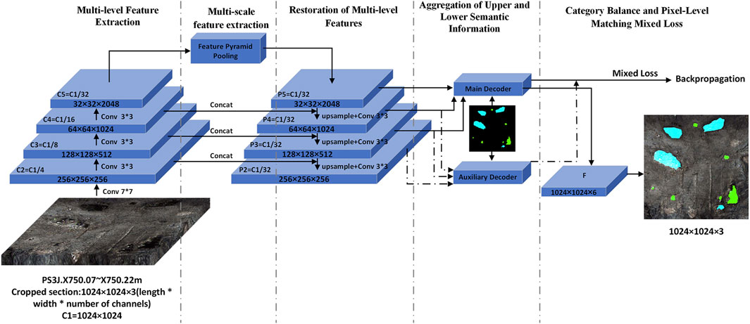
FIGURE 2. Framework of MFAPNet.

4.1 Multi-level feature extraction

The extraction of multi-level features enables the model to extract high-order attributes from raw data, including edges, textures, shapes, and object components. The in-depth analysis and representation of intricate data structures empower the model to comprehend and depict detailed elements contained in input images. Through the extraction of multi-level features, the model can discern complex and abstract attributes and grasp data variances and non-linear interrelationships.

For deep neural networks, key challenges like the gradient vanishing and exploding problem are solved through the incorporation of regularized initialization and intermediary regularization layers, notably, Batch Normalization (Ioffe and Szegedy, 2015). Degradation quandaries inherent to deep networks are addressed with residual modules. As illustrated in Figure 3, with an input denoted by x and its corresponding residual function F(x), the output generated by the residual module is defined as x + F(x). With this module, the input x is subjected to the transformation F and then the residual information is extracted to augment the foundational input x. This addition process indicates skip connections, namely, the integration of residual data with the original input, and can ensure refinement and adjustment. Such an architecture empowers neural networks to internalize the identity function I(x) = x throughout the training process. If it is the optimal solution, the module can discern an almost null residual, thereby retaining the integrity of the initial input. Conversely, in the presence of substantial discrepancies, the module can ascertain a more pronounced residual to refine the input data.

FIGURE 3

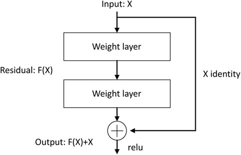
FIGURE 3. Residual module.

As depicted in Figure 2; Figure 4, a segment from PS3J.X750.07-X750.22 is selected. With the input data of 1024×1024×3 (C1 = 1024×1024), based on the ResNet primary feature extraction network, through 7x7 convolution, the feature map C2 with a quarter of its original size is obtained and its channels is increased to 256. Subsequently, the image undergoes a series of three analogous operations employing three 3x3 residual convolution to produce three distinct feature maps labeled as C3, C4, and C5. Their sizes respectively decrease to 1/8, 1/16, and 1/32 of the original size, whereas their channel increases to 512, 1024, and 2048.

FIGURE 4

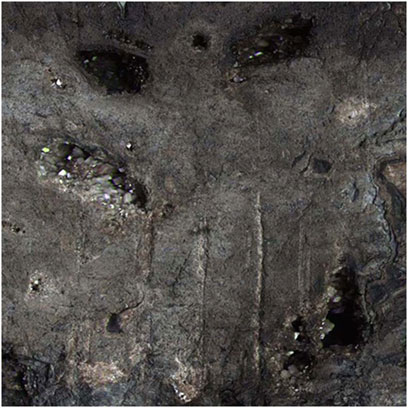
FIGURE 4. Segment from PS3J.X750.07-X750.22m.

4.2 Multi-scale feature extraction

In the fields of deep learning and computer vision, multi-scale feature extraction refers to capturing features from the data at different scales for the comprehensive information acquisition. The feature extraction approach performs well in handling the data at different scales, such as images, videos, and texts. The data at different scales correspond to structures and features with spatial or temporal scales. Harnessing multi-scale features allows models to encompass both granular and macroscopic characteristics and obtain a more profound comprehension of the data.

In deep convolutional networks, the realized receptive field is often far shorter than theoretical expectations. To counteract this discrepancy, the pyramid pooling module from PSPNet (Zhao et al., 2017) is incorporated into the terminal layer of the primary network. This integration ensures pyramid-style multi-scale feature extraction, as illustrated in Figure 5 and expressed as:

$P5=Con{v}_{3\times 3}\left[{\displaystyle \sum _{i=1\times 1、2\times 2、3\times 3、6\times 6}^{U\mathrm{p}sample、Concat}}AvgP{\text{ool}}_i+{\text{Conv}}_{1\times 1}\left(C5\right)\right](1)$

FIGURE 5

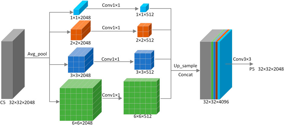
FIGURE 5. Pyramid pooling module (PPM).

Through average pooling (AvgPool) with four distinct sizes, the C5 layer captures multi-scale semantic feature insights. Subsequently, through the 1x1 convolution, the channels are reduced to a quarter of their initial size. After these features are upsampled to their original dimensions, they are concatenated and processed with the 3x3 convolution so as to integrate the multi-scale features into P5 and obtain comprehensive global information.

4.3 Restoration of multi-level features

To acquire multi-level semantic information with minimal interference, high-level features are realigned to the spatial resolution of the low-level features. This realignment, as expressed in Eq. 2, facilitates the restoration of features.

$P_{\mathrm{i}}={\text{Conv}}_{1\times 1}\left(Upsample\left(P_{i-1}\right)+C_i\right),i=\mathrm{4,3,2}(2)$

The feature layer P5 is upsampled to match the resolution of the C4 feature layer. Subsequently, it is concatenated and convolved with the C4 feature map to yield P3. This operation is reiterated twice to obtain the feature maps across various semantic levels: P5, P4, P3, and P2. By integrating high-level semantic information with low-level features, the details and semantics in high-resolution images are captured. This integration enhances the performance of the model in intricate tasks like object detection and image segmentation through a robust and precise feature representation.

4.4 Aggregation of upper and lower semantic information

As the depth of a convolutional neural network increases, the semantic information extracted at each layer becomes increasingly rich, so that more global features are obtained. Analogously, the human visual system operates in a comparable way, in which global features as initial features are progressively refined for precise decision-making. Such a hierarchical processing way of features allows the sequential consideration of various levels of abstract features during data processing so as to facilitate a more comprehensive understanding and representation of intricate data, as expressed in Eqs 3, 4:

$F=Con{v}_{3\times 3}\left({\displaystyle \sum _{i=2、3、4、5}^{U\mathrm{p}sample、Concat}}{P}_i\right)(3)$

$F_2=Con{v}_{3\times 3}\left[U\mathrm{p}sample\left(P4\right)\right](4)$

The main decoding head receives (P5, P4, P3) as the input, whereas the auxiliary decoding head processes (P4, P3, P2). After the obtained feature maps are restored to their original dimensions through upsampling, these features are concatenated into coherent feature maps. A subsequent 3x3 convolutional operation is performed to modulate the channel count so as to obtain the main and auxiliary feature segmentation maps, respectively denoted as F and F2. F is then superimposed onto the original image to generate the final prediction. The primary and auxiliary losses are amalgamated through weighted summation and applied in backpropagation for model optimization.

4.5 Class balance and pixel-level matching mixed loss

To deal with the unequal class distribution and ensure the matching between prediction results and actual labels, a class-balanced and pixel-level matched hybrid loss function is used in the study. The mixed loss function considering class-balanced cross-entropy loss and Dice Loss (Li X et al., 2019) is adopted:

$CBCED\_LOSS=\alpha *CBCE\_Loss+\beta *Dice\_Loss(5)$

where CBCE_Loss denotes the class-balanced cross-entropy loss; Dice_Loss indicates Dice loss; CBCED_LOSS considers both class imbalance and pixel-level matching; α and β can be tuned according to the properties of tasks and datasets for the balance between the two loss types. In our work, a large weight is assigned to Dice Loss for pixel-level matching. A ratio of 1:3 (α=1 and β=3) is adopted. For CBCE_LOSS, it is assumed that C distinct classes exist and a weight, w_i, is assigned to a class and indicates its significance (i is the class index). Given a collection of samples, each sample has a true label Y and a predicted probability distribution P from the model. Then, the class-balanced cross-entropy loss is expressed as:

$CBCE\left(P,Y\right)=-{\sum }_{\mathrm{i}=1}^C{w}_i\times Y_i\times \mathit{log}\left(P_i\right)(6)$

where Y_i is the i-th element of the true label; P_i is the i-th element from the predicted probability distribution; w_i is the weight associated with the class. These weights can be modulated according to the importance of different classes so as to further address class imbalances. The ultimate loss is the mean loss across all samples:

$CBCE\left(P,Y\right)=\frac{1}{N}{\displaystyle \sum _{\mathrm{n}=1}^N}CBCE\left(P\left(s_n\right),Y_n\right)(7)$

where N indicates the total number of samples. The class-balanced cross-entropy loss allows different importance levels for different classes and can be used to deal with many computer vision tasks, especially class-imbalanced problems.

For Dice Loss, two sets (A and B) are considered. The size of their intersection is represented by $\left|A\cap B\right|$ and the size of their union is depicted as $\left|A\cup B\right|$ Then, Dice Loss can be defined as:

$DiceLoss=1-\frac{2*\left|A\right|\cap \left|B\right|}{\left|A\right|+\left|B\right|}(8)$

where $\left|A\right|$ and $\left|B\right|$ respectively indicate the sizes of sets A and B; $\left|A\cap B\right|$ represents the size of their intersection. Dice Loss value is between 0 and 1. The smaller the value is, the less the consistency between the predicted and actual segmentation results is.

In tasks involving semantic segmentation, Dice Loss is often used to indicate the resemblance between predicted and actual segmentation outcomes. Unlike cross-entropy loss, Dice Loss is focuses on pixel-level matching and performs better in dealing with class imbalances.

The gradient data from both primary and auxiliary losses calculated from F and F2 can be used to update network parameters through backpropagation. During backpropagation, the gradient information from the loss function flows backwards through network layers so as to guide weight adjustment. In this way, the model is adapted to training data and yields precise predictions for new data.

5 Experiments

5.1 Experimental parameter setting

To guarantee the precision of experimental results, the control variates method was used. In this method, all parameters remained constant except that the test variable was changed. Our experiments were executed on Windows 11 22H2 Professional Edition system and NVIDIA RTX A6000 48G GPU was used for training. The size of input images was 1024×1024 (Table 1).

TABLE 1

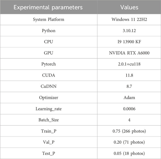
TABLE 1. Experimental parameter setting.

The principal evaluation metric was mIoU. Additionally, Accuracy (Acc) and F-score (Wang et al., 2020) were used to indicate the performance of the network model in defect segmentation. mIoU is the average IoU value of all images or segmentation results. IoU (Intersection over Union) quantifies the relationship between the intersection and union areas of segmentation results and actual results as follows:

$IoU=\frac{Intersection}{Union}(9)$

Accuracy is the ratio of the number of the pixels correctly classified by the model to the total number of pixels:

$Accuracy=\frac{NumberofCorrectlyClassifiedPixels}{TotalNumberofPixels}(10)$

F-Score is the weighted average of precision and recall and can be used to evaluate the comprehensive efficacy of the classification model. F-Score indicates the balance between model precision and recall and can be expressed as:

$Fscore=\frac{2\cdot Precision\cdot Recall}{Precision+Recall}(11)$

5.2 Experimental dataset setting

In this study, the data of the core samples from the deep carbonate rock reservoir of the Dengying Formation located in Penglai Gas Area of Sichuan Basin. After screening the core data from various wells, FracturesHoleAlgae Dataset (CHA355) was derived. This dataset contained 266 training images, 71 validation images, and 18 testing images. As shown in Figure 6, the name of an image is composed of well sequence, depth range, and core number. The dimension of each image is 1024×1024 pixels and the sections indicate the representative areas from the initial core rolling scan images.

FIGURE 6

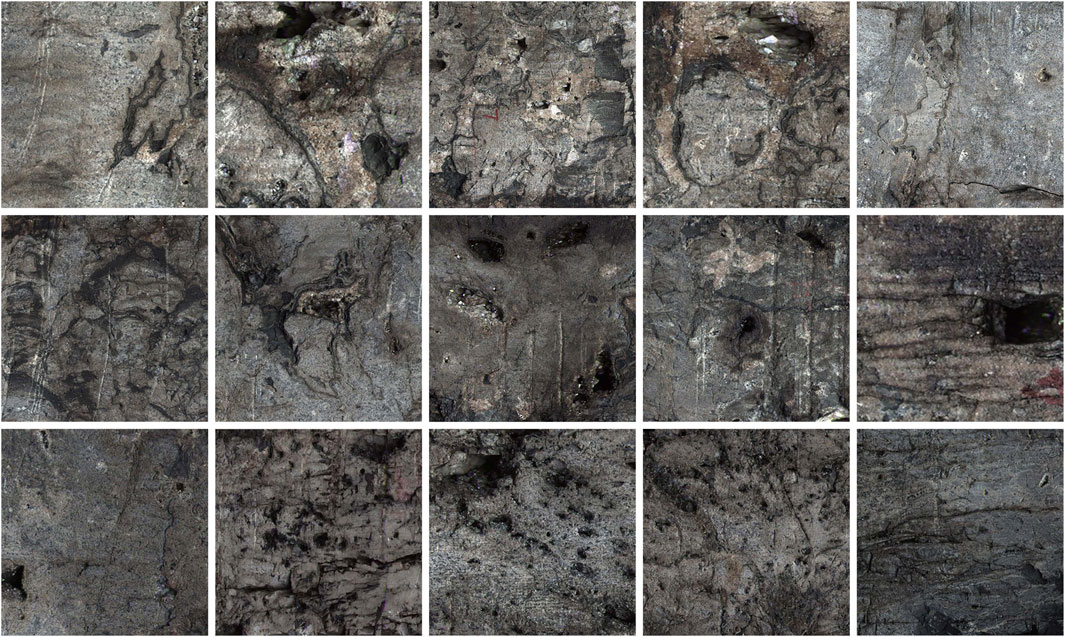
FIGURE 6. Partial original images in the dataset.

Figure 7 shows various colors for segmentation. Green indicates unfilled dissolved holes; cyan indicates filled dissolved holes; red indicates open fractures; yellow denotes filled fractures; purple indicates algae; black indicates the background. These annotated images are displayed in VOC format.

FIGURE 7

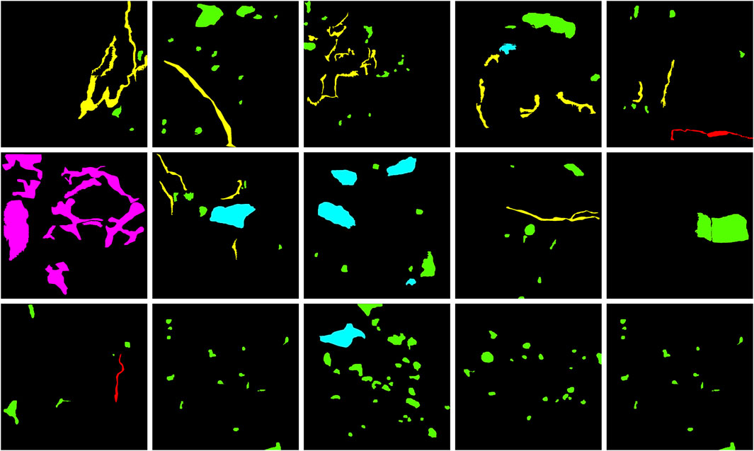
FIGURE 7. Partial labeled images in the dataset.

5.3 Comparison of experimental results obtained with different algorithms

In the section, the proposed MFAPNet was compared with renowned segmentation techniques such as FCN (Long et al., 2015), UNet, PSPNet, DeepLabV3 (Chen et al., 2017), and UperNet (Xiao et al., 2018). In FCN, the fully connected layer is replaced with a convolutional one so that it is feasible to input an image in any size. In UNet with an encoder-decoder design, an encoder is used to grasp image information, whereas the decoder is used to generate pixel-level segmentation results. In PSPNet, with a pyramid pooling module, the data at different scales are extracted. In DeepLabV3, dilated convolution is used to widen the receptive field and thus grasp more information. UperNet integrates UNet with pyramid structure and can enhance the multi-scale performance.

The segmentation results from CHA355 dataset are presented in Table 2. The mIoU value of MFAPNet was 14.49%, 7.53%, 5.03%, 6.85%, and 0.65% larger than that of FCN, UNet, PSPNet, DeepLabV3, and UperNet, respectively. Similarly, its mAcc was the mentioned models by 19.99%, 13.38%, 5.14%, 12.19%, and 3.06% larger than that of FCN, UNet, PSPNet, DeepLabV3, and UperNet, respectively. The mFscore of MFAPNet was 16.45%, 7.85%, 4.6%, 8.1%, and 0.65% larger than that of FCN, UNet, PSPNet, DeepLabV3, and UperNet, respectively. The mPrecision, of MFAPNet was 2.3% larger than that of FCN, equal to that of UNet, and reached 99.93%, 91.77%, and 97.30% of that of PSPNet, DeepLabV3, and UperNet, respectively. In conclusion, although MFAPNet lagged behind PSPNet, DeepLabV3, and UperNet in terms of mPrecision, its overall performance was better than that of the other five models in image segmentation.

TABLE 2

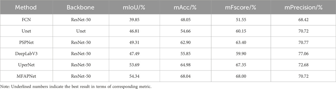
TABLE 2. Comparison of the results obtained with different algorithms from CHA355 dataset.

The segmentation results obtained with various algorithms from VOC2012 dataset are shown in Table 3. The mIoU value of MFAPNet was 7.62%, 4.57%, 2.71%, 3.30%, and 0.04% larger than that of FCN, UNet, PSPNet, DeepLabV3, and UperNet, respectively. The mAcc value of MFAPNet was respectively 4.35%, 0.58%, and 0.63% larger than that of FCN, PSPNet, and DeepLabV3 and 1.62% and 0.57% smaller than that of Unet and UperNet. The mFscore of MFAPNet was 6.06%, 2.73%, 1.85%, 2.21%, and 0.07% larger than that of FCN, UNet, PSPNet, DeepLabV3, and UperNet, respectively. The mPrecision of MFAPNet was 5.25%, 7.19%, 3.16%, 3.9%, and 0.576% larger than that of FCN, UNet, PSPNet, DeepLabV3, and UperNet, respectively.

TABLE 3

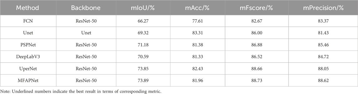
TABLE 3. Comparison of the results obtained with different algorithms from VOC2012 dataset.

5.4 Comparison of different loss functions

In this section, CBCED_Loss was compared with other loss functions: CrossEntropyLoss, DiceLoss, FocalLoss (Lin et al., 2017) and TverskyLoss (Milletari et al., 2016). CrossEntropyLoss quantifies the discrepancy between the predicted classification results of the model and actual labels and is commonly applied in multi-class classification scenarios. DiceLoss indicates the consistency of overlapping regions between predictions and actual labels and can address data imbalances. FocalLoss was designed to mitigate the class imbalance issue. In FocalLoss, in order to reduce the influence of easily classified samples, a larger weight is assigned to the samples which are difficult to be classified. In TverskyLoss, weight can be adjusted in the loss calculation so as to reach the balance between precision and recall.

Table 4 presents the results from CHA355 dataset. The mIoU value of CBCED_Loss was 1.76%, 4.41%, 3.45%, and 7.53% larger than that of CrossEntropyLoss, DiceLoss, FocalLoss, and TverskyLoss, respectively. Similarly, the mAcc value of CBCED_Loss was 3.29%, 4.14%, 4.48%, and 13.38% larger than that of CrossEntropyLoss, DiceLoss, FocalLoss, and TverskyLoss, respectively. The mFscore of CBCED_Loss was 1.56%, 4.15%, 4.09%, and 7.85% larger than that of CrossEntropyLoss, DiceLoss, FocalLoss, and TverskyLoss, respectively. The mPrecision, value of CBCED_Loss was 4.39% and 1.05% larger than that of DiceLoss and FocalLoss, equal to that of TverskyLoss, and 2.00% smaller than that of CrossEntropyLoss, respectively. In summary, even though the mPrecision of CBCED_Loss was slightly smaller than that of CrossEntropyLoss, its overall performance was more uniform and stable than the other four loss functions.

TABLE 4

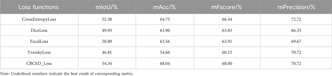
TABLE 4. Comparison of the results obtained with different loss functions from CHA355 dataset.

5.5 Training process and results

As shown in Figure 8, both mAcc (blue curve) and mIoU (orange curve) firstly display the consistent rising and stable trend and then converge. Notably, due to the utilization of pre-trained parameters from ImageNet-22K in this study, mFscore (orange curve) was large in the initial training phase. Then, these parameters were increasingly consistent with the dataset used in this study. After 4,000 iterations, the model was fully consistent with the parameters from the pre-trained model. The mFscore firstly increased and then converged.

FIGURE 8

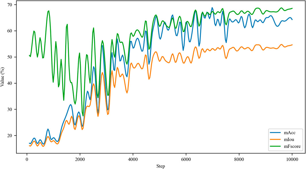
FIGURE 8. Training process.

As shown in Table 5, the model exhibited the optimal performance in recognizing filled fractures in the image except the background region. It distinguished open fractures from filled fractures better, but it could not distinguished unfilled holes from filled holes well. Furthermore, the model identified algae well.

TABLE 5

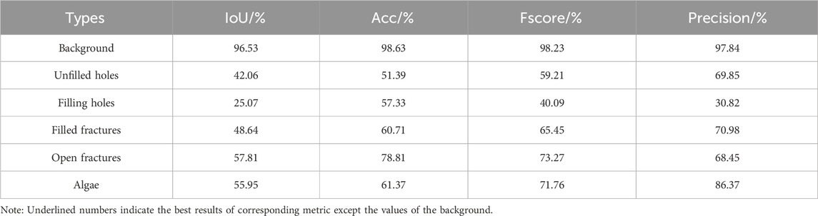
TABLE 5. Comparison of the results obtained with MFAPNet from CHA355 dataset.

5.6 Comparison of visualization results

Figure 9 shows the segmentation results obtained with various network models from CHA355 dataset. In the first row, due to the heterogeneity in algae features and considerable interference, the algal segmentation results of various network models were different. Notably, MFAPNet identified discrete algal layers better than other algorithms. The second row, characterized by white scratch interference, revealed that MFAPNet, PSPNet, and UperNet discerned filled fractures. In the third row, when obvious fractures could be observed without other interferences, every network model segmented the fractures well. In the fourth row, when mixed filled and unfilled holes could be observed, all models yielded false identification results of some holes. However, MFAPNet and UperNet could discriminate unfilled holes from filled holes. On the whole, the MFAPNet model developed in this study offered better segmentation results, outperformed other models in dealing with interferences and distinguishing filled regions from unfilled regions.

FIGURE 9

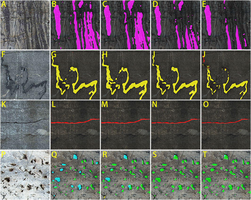
FIGURE 9. (A, F, K, P) are original images; (B, G, L, Q) are prediction results of MFAPNet; (C,H,M,R) are prediction results of PSPNet; (D, I, N, S) are prediction results of UperNet; (E, J, O, T) are prediction results of FCN. (A): Dominated by developmental algae, the algal layers are clearly visible; (F): Dominated by filled fractures, they pervade the entire image; (K): In the middle of the image, there is a open fracture that runs through the entire image; (P): Dominated by dissolved holes, some are unfilled while others are filled.

6 Application

In the study, the deep carbonate rock reservoir of the Dengying Formation in the Penglai Gas Field, Sichuan Basin was selected for porosity calibration. Figure 10A shows the original core rolling scan image of the segment PS9J.X977.10-X977.22. A representative area was selected (Figure 10B). This selected image was then input into MFAPNet to output the prediction result (Figure 10C).

FIGURE 10

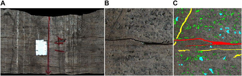
FIGURE 10. Comparison diagram: (A) original core rolling scan photo; (B) selected area; (C) predicted results.

Unfilled structures have no geological significance for oil and gas exploration, so only these parts were considered for further analysis. The porosity is calculated as:

$Porosity=\frac{np.sum\left(M\text{ask}==\mathrm{n}\right)}{M\text{ask}.size}\times 100\%(12)$

where $M\text{ask}$ indicates the MFAPNet’s prediction output; $np.sum\left(M\text{ask}==\mathrm{n}\right)$ indicates the summation of the values of the pixels with the predicted result equal to n (the value of unfilled fractures and holes); $M\text{ask}.size$ indicates the cumulative value of the pixels in the predicted image. With Eq. 12; Figure 10C, the proportion of unfilled holes was calculated to be 4.48% and the proportion of open fractures was 2.41%. Consequently, core porosity for the segment shown in Figure 10A was 6.89%.

With this method, the porosity of PS13 core was determined, as illustrated in the porosity histogram (the sixth track in Figure 11). Subsequent image segmentation enabled the extraction of wellbore imaging porosity (the third track), in which the wellbore imaging porosity curve was computed with a window length of 1 ft and a step of 0.1 in. When the logging tool’s button electrode was close to an unfilled natural fracture, the resistivity of the drilling fluid within fractures was substantially lower than that of adjacent rock, thus leading to the large current of the electrode. As a result, the apparent width of fractures in imaging results was several times of their actual width (Nian et al., 2021). This phenomenon might also lead to the enlarged boundaries of dissolved holes. For a more precise representation of porosity, the curve was mathematically adjusted in this study. The refined curve was well consistent with the core porosity histogram. The curves in Figure 11 (sixth track) revealed that the porosity derived from wellbore imaging was 1.5–3 times of that obtained from core rolling scan images. Moreover, the difference increased with the decrease in porosity. This result, to some extent, reveals the correlation between the wellbore image logging data and the actual characteristics of the Dengying Formation in the Penglai Gas Field of the Sichuan Basin. It also provides a certain basis for the subsequent logging evaluation of the formation.

FIGURE 11

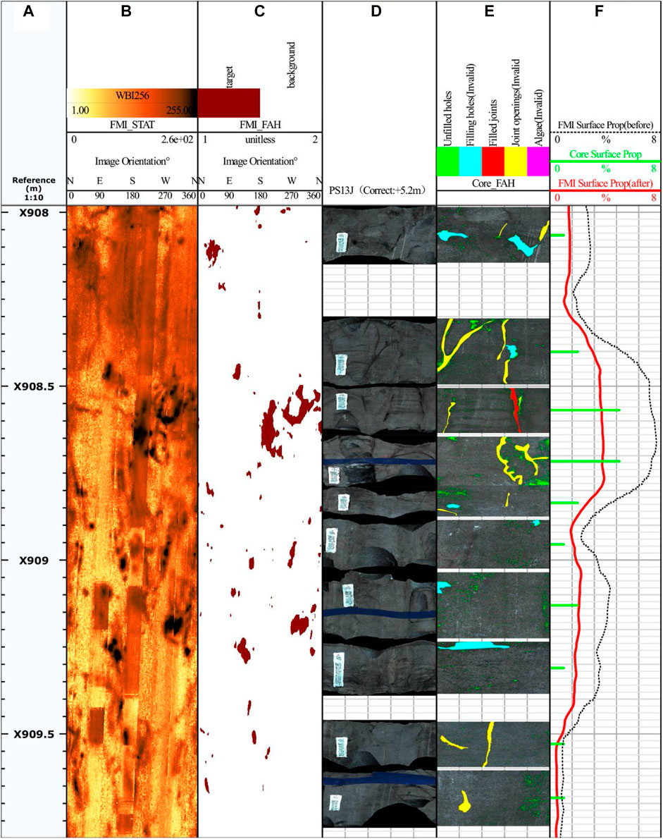
FIGURE 11. PS13J Comparison chart. (A) signifies a depth trace utilized for depth indexing. (B) represents a statically enhanced image derived from the Wellbore image. (C) displays an image capturing fractures and holes. (D) depicts a core rolling scan image at the specified depth. (E) denotes the outcomes following model segmentation. In (F), a comparison of surface porosity is presented, with the black curve representing the surface porosity calculated based on the image of fractures and holes from the third trace. The green discrete columnar points correspond to the surface porosity derived from the respective core rolling scan image, and the red curve portrays the predicted core surface porosity post-calibration.

7 Conclusion

1. Based on the detailed descriptions of the core rolling scan images of the deep carbonate rock reservoir of the Dengying Formation in Penglai Gas Field, Sichuan Basin, we successfully acquired the distinct features of various fractures and holes and formulated a robust classification framework for these types. We highlighted three primary challenges in segmenting datasets comprising fractures, holes, and algae: variance in feature scales, class imbalance, and a limited dataset number with larger samples.

2. After the introduction of SAM segmentation model, we facilitated semi-automatic delineation of the target regions (fractures and holes) from the background in images and markedly accelerated the geological dataset compilation process.

3. We developed the MFAPNet semantic segmentation deep learning model, which ensured swift and high-fidelity intelligent recognition of fracture types as well as the quantitative analysis of fractures and holes.

4. We explored the porosity of wellbore imaging results and core rolling scan images and further validated the calibration relationship between electric imaging results and core rolling image porosity.

Data availability statement

The datasets presented in this study can be found in online repositories. The names of the repository/repositories and accession number(s) can be found below: https://github.com/zyng886/MFAPNet.

Author contributions

QL: Funding acquisition, Writing–review and editing. YW: Funding acquisition, Writing–review and editing. YZ: Writing–original draft. BX: Data curation, Investigation, Writing–review and editing. YJ: Data curation, Investigation, Writing–review and editing. LC: Data curation, Investigation, Writing–review and editing. MT: Data curation, Writing–review and editing. FL: Funding acquisition, Methodology, Resources, Writing–review and editing.

Funding

The author(s) declare financial support was received for the research, authorship, and/or publication of this article. The authors declare financial support was received for the research, authorship, and/or publication of this article. This work was financially supported by the National Natural Science Foundation of China (Grant 41402118) and also supported by Chongqing Municipal Education Commission Science and Technology Research Projects (KJZD-K202301508 and KJON202301535).

Acknowledgments

The authors are grateful to Yuejiao Liu for his invaluable assistance with scanning the sample.

Conflict of interest

Authors QL, YW, BX, and LC were employed by PetroChina Southwest Oil & Gas Field Company.

The remaining authors declare that the research was conducted in the absence of any commercial or financial relationships that could be construed as a potential conflict of interest.

Publisher’s note

All claims expressed in this article are solely those of the authors and do not necessarily represent those of their affiliated organizations, or those of the publisher, the editors and the reviewers. Any product that may be evaluated in this article, or claim that may be made by its manufacturer, is not guaranteed or endorsed by the publisher.

References

Chen, L. C., Papandreou, G., Schroff, F., and Adam, H. (2017). Rethinking atrous convolution for semantic image segmentation. arXiv preprint arXiv:1706.05587. Available at: https://doi.org/10.48550/arXiv.1706.05587.

Google Scholar

Chen, Z. M., Tang, X., Liang, G. D., and Guan, Z. H. (2023). Identification and comparison of organic matter pores in shale scanning electron microscope images based on deep learning. Earth Sci. Front. 2023 (03), 208–220. doi:10.13745/j.esf.sf.2022.5.45

CrossRef Full Text | Google Scholar

Delhomme, J. P. (1992). “A quantitative characterization of formation heterogeneities based on borehole image analysis,” in Trans 33rd Symp Soc Prof Well Log Analysts, Oklahoma City, Oklahoma, June 1992. Paper T.

Google Scholar

Everingham, M., Van Gool, L., Williams, C. K. I., Winn, J., and Zisserman, A. (2012). The PASCAL visual object classes challenge 2012 (VOC2012) results.

Google Scholar

Hall, J., Ponzi, M., Gonfalini, M., and Maletti, G. (1996). “Automatic extraction and characterization of geological features and textures from borehole images and core photographs,” in Trans 37th Symp Soc Prof Well Log Analysts, New Orleans, Louisiana, June 1996. Paper CCC.

Google Scholar

He, K., Zhang, X., Ren, S., and Sun, J. (2016). “Deep residual learning for image recognition,” in Proceedings of the IEEE conference on computer vision and pattern recognition, Las Vegas, NV, USA, 27-30 June 2016, 770–778.

CrossRef Full Text | Google Scholar

Ioffe, S., and Szegedy, C. (2015). “Batch normalization: accelerating deep network training by reducing internal covariate shift,” in International conference on machine learning, 448–456. pmlr.

Google Scholar

Kirillov, A., Mintun, E., Ravi, N., Mao, H., Rolland, C., and Gustafson, L. (2023). Segment anything. arXiv preprint arXiv:2304.02643. Available at: https://doi.org/10.48550/arXiv.2304.02643.

Google Scholar

Lai, F. Q. (2011). Study on the processing and interpretation methods of electric imaging logging. Beijing: China University of Petroleum.

Google Scholar

Li, B. T., Wang, Z. Z., Kong, C. X., Jiang, Q. P., Wang, W. F., Lei, X. H., et al. (2019). New method for intelligent identification of fractures based on imaging logging. Well Logging Technol. 2019 (03), 257–262. doi:10.16489/j.issn.1004-1338.2019.03.007

CrossRef Full Text | Google Scholar

Li, Z. H., Zhang, X., Luo, L., Mao, Y. X., and Li, M. (2016). Automatic identification and parameter calculation of holes in carbonate rock with a complex background. Fract. Oil Gas Fields 2016 (03), 314–323.

Google Scholar

Lin, T. Y., Goyal, P., Girshick, R., He, K., and Dollár, P. (2017). “Focal loss for dense object detection,” in Proceedings of the IEEE international conference on computer vision, Venice, Italy, 22-29 October 2017, 2980–2988.

CrossRef Full Text | Google Scholar

Li X, X., Sun, X., Meng, Y., Liang, J., Wu, F., and Li, J. (2019). Dice loss for data-imbalanced NLP tasks. arXiv preprint arXiv:1911.02855. Available at: https://doi.org/10.48550/arXiv.1911.02855.

Google Scholar

Long, J., Shelhamer, E., and Darrell, T. (2015). “Fully convolutional networks for semantic segmentation,” in Proceedings of the IEEE conference on computer vision and pattern recognition, Boston, MA, USA, 07-12 June 2015, 3431–3440.

CrossRef Full Text | Google Scholar

Ma, Y. S., Cai, X. Y., Li, H. L., Zhu, D. Y., Zhang, J. T., Yang, M., et al. (2023). New understanding of the development mechanism of deep-super deep carbonate reservoirs and the direction of ultra-deep oil and gas exploration. Geol. J. 30.06 (2023), 1–13. doi:10.13745/j-esf.sf.2023.2.35

CrossRef Full Text | Google Scholar

Ma, Y. S., Cai, X. Y., Yun, L., Li, Z. J., Li, H. L., Deng, S., et al. (2022). Exploration and development practices and theoretical and technical advancements in the Shunbei ultra-deep carbonate oil and gas field in the Tarim Basin. Petroleum Explor. Dev. 01, 1–17.

CrossRef Full Text | Google Scholar

Ma, Y. S., He, Z. L., Zhao, P. R., Zhu, H. Q., Han, J., You, D. H., et al. (2019). New progress in the formation mechanism of deep-super deep carbonate reservoirs. Acta Pet. Sin. 2019 (12), 1415–1425.

CrossRef Full Text | Google Scholar

Milletari, F., Navab, N., and Ahmadi, S. A. (2016). “V-net: fully convolutional neural networks for volumetric medical image segmentation,” in 2016 fourth international conference on 3D vision (3DV), Stanford, CA, USA, 25-28 October 2016, 565–571.

CrossRef Full Text | Google Scholar

Nian, T., Wang, G. W., Fan, X. Q., Tan, C. Q., Wang, S., Hou, T., et al. (2021). Progress in fracture and cave interpretation evaluation based on imaging logging. Geol. Rev. 2021 (02), 476–488. doi:10.16509/j.georeview.2021.02.016

CrossRef Full Text | Google Scholar

Ren, X. F., Wen, X. F., Lin, W. C., Liu, A. P., Yu, B. C., and Cai, F. (2023). Quantitative characterization technology and its application based on micro-resistivity imaging logging of tight carbonate rock pore space parameters. Well Logging Technol. 47 (01), 48–54.

Google Scholar

Ronneberger, O., Fischer, P., and Brox, T. (2015). “U-net: convolutional networks for biomedical image segmentation,” in Medical Image Computing and Computer-Assisted Intervention–MICCAI 2015: 18th International Conference, Munich, Germany, October 5-9, 2015, 234–241. Proceedings, Part III 18.

CrossRef Full Text | Google Scholar

Tian, F., and Zhang, C. G. (2010). Fracture identification technology of electric imaging logging data and its application. J. Geophys. Eng. 7 (6), 723–727.

Google Scholar

Wang, L., Shen, J. S., Heng, H. L., and Wei, S. S. (2021). Research on automatic identification and separation of fractures and caves in electric imaging logging based on path morphology and sine function family matching. Petroleum Sci. Bull. 6 (03), 380–395.

Google Scholar

Wang, Q., Wu, B., Zhu, P., Li, P., Zuo, W., and Hu, Q. (2020). “ECA-Net: efficient channel attention for deep convolutional neural networks,” in Proceedings of the IEEE/CVF conference on computer vision and pattern recognition, 11534–11542.

CrossRef Full Text | Google Scholar

Xiao, T., Liu, Y., Zhou, B., Jiang, Y., and Sun, J. (2018). “Unified perceptual parsing for scene understanding,” in Proceedings of the European conference on computer vision (ECCV), 418–434.

CrossRef Full Text | Google Scholar

Zhao, H., Shi, J., Qi, X., Wang, X., and Jia, J. (2017). “Pyramid scene parsing network,” in Proceedings of the IEEE conference on computer vision and pattern recognition, 2881–2890.

CrossRef Full Text | Google Scholar

Zou, C. N., Du, J. H., Xu, C. C., Wang, Z. C., Zhang, B. M., Wei, G. Q., et al. (2014). Formation distribution, resource potential, and exploration discoveries of the Sinian-Cambrian in the Sichuan Basin. Petroleum Exploration and Development.

Google Scholar