Multi-data settlement prediction along a road section integrating InSAR and coastal subsurface information with data assimilation

This paper presents a novel approach to examining the impact of soil settlement and its spatial distribution on infrastructure. The study focuses on a specific road section in the Friesland coastal plain in the north of the Netherlands, investigating how the Holocene coastal subsurface architecture influences settlement patterns. Our study underscores the importance of integrating multiple datasets, providing data at varying resolutions. The road segment traverses lithostratigraphical units, which include tidal channel and tidal flat deposits, overlaying an older tidal basin system and intercalated peat beds. Through data assimilation of a settlement model optimized with InSAR measurements, we have identified settlement heterogeneities that can be explained by combining high-resolution variations in lithology with gradual changes in lithostratigraphy. This was accomplished by utilizing a medium-resolution model (MRM) based on borehole descriptions and a high-resolution data (HRD) approach based on cone penetration tests along the road. The HRD method proved more effective in capturing abrupt changes in lithology between channel structures, while the MRM provided a continuous representation of the lithostratigraphic setting of the area. Our study demonstrates that subsurface heterogeneities have significant implications for subsidence along roads. Settlement rates increase from 2–4 mm/year towards 9 mm/year along the road section, resulting in a differential settlement of more than 5 mm/year over a distance of less than a kilometer. This is primarily attributed to variations in lithostratigraphy. Overall, this new innovative approach offers a practical and cost-effective solution for predicting subsidence due to settlement, eliminating the need for expensive laboratory tests. By integrating lithology and lithostratigraphy, more efficient road maintenance and management become possible.

1 Introduction

Subsidence poses a significant challenge to society, putting regions at risk of high cost and hazardous situations (Candela and Koster, 2022; Shi et al., 2022). Especially subsiding low-lying coastal areas with soft soils are prone to floods and damage inflicted to buildings and infrastructure (Törnqvist et al., 2008; Abidin et al., 2011; Ohenhen and Shirzaei, 2022). Yet, a not well studied consequence of subsidence is the differential settlement of roads. Roads play a vital role in connecting communities, facilitating socio-economic activities and ensuring the overall functionality of societies. Differential subsidence through settlement inflicts damage to roads, especially in areas with a highly heterogeneous and compressible coastal subsurface (Khoshlahjeh Azar et al., 2022; Gee et al., 2019; Ngan-Tillard et al., 2010; Polcari et al., 2019). Therefore, it would be a critical step forward for road-operators to be able to forecast road settlement, and subsequently mitigate identified hazards.

The costs associated with road maintenance as a result of settlement are significant. For example, the maintenance costs related to road settlements in the peat-rich coastal plains of the Netherlands are estimated at than 100 million euros per year (Van den Born et al., 2016). This is about 10% of the total national budget for road maintenance (Rijksoverheid, 2023). Similarly, the costs for infrastructure maintenance related to settlement in the urban districts of Semerang and Demak, coastal Indonesia, are projected to increase to 50–100 million euros per city over the course of 20 years (Mahya et al., 2021). In Delhi millions of rupees are spend on road maintenance of a subsiding road of 7.5 km long (Garg et al., 2022). In general, settlement is one of the main drivers of increasing maintenance costs for delta cities all around the world (Bucx et al., 2015), emphasizing the global significance of mitigating this issue.

Differential road settlement is often the result of variation in subsurface composition, primarily short-spatial-scale variation in soil types and larger-spatial-scale variation in geological features (Ngan-Tillard et al., 2010). Clay and peat beds play an especially important role because of their high compressibility (Koster et al., 2016; Low et al., 2019). Knowledge and predictability of settlement patterns is key in developing strategies to prolong the integrity of coastal roads. To achieve this, it is important to develop a generic approach that captures the behavior of the subsurface under different loading conditions. Furthermore, non-destructive and widely available data are paramount for broad application.

Studies on road settlement often rely on a qualitative analysis of monitoring data (e.g. Yu et al., 2013a; Mazzanti, 2017; Polcari et al., 2019; Du et al., 2022). These studies assess settlement and its variance along road infrastructures and describe potential associations relations with subsurface architecture or human interventions, such as additional loading and engineering works. However, without a quantitative understanding of settlement, it becomes challenging to forecast future settlement patterns and identify hazardous zones. Studies that quantitatively model settlement primarily rely on laboratory or in-situ measurements (e.g. Yu et al., 2013b; Cui et al., 2014; Lu et al., 2018). Such an approach requires the use of often costly instruments to collect and measure data at each studied section of the infrastructure.

The collection and interpretation of Interferometric Synthetic Aperture Radar (InSAR) data is a cost-effective and non-destructive technology for surface displacement estimation, because it does not require additional field monitoring of individual road sections. Previous studies have shown that coastal plain subsurface composition can be correlated to measured surface displacements with modeled settlement through data assimilation techniques (Peduto et al., 2016; Peduto et al., 2020; Verberne et al., 2023a). Peduto et al. (2016, Peduto et al., 2020) for instance, used Persistent Scatter InSAR (PS-InSAR) on coastal road sections in the Netherlands, utilizing coherent radar reflections from strong scatterers for settlement measurements. These measurements were subsequently used in back analysis with a data assimilation approach to optimize settlement estimates obtained from conventional monitoring data.

We have adopted a settlement modeling approach for road infrastructure based on displacements derived from InSAR to estimate key parameters required for settlement predictions with data assimilation. We applied this to a road section in the soft-soil Friesland coastal plain in the north of the Netherlands (Figure 1). We address the following research questions: 1) can the differential settlement along the road section be explained by integrating InSAR and subsurface data? 2) What is the influence of short spatial scale and larger spatial scale subsurface composition on the settlement profiles?

FIGURE 1

FIGURE 1. Four maps that provide information about the study area. Map (A) shows the location of the Netherlands and highlights the Holocene thickness, which increases towards the northwest and exhibits channel structures. The research area is located within a northern sea ingression tidal channel system. The Holocene thickness is derived from the GeoTOP model (TNO-GSN, 2023). Map (B) is a close-up view of the region around the area. Here the medieval tidal inflow channel is highlighted. The background gives an indication of the topographic map of the Netherlands, the AHN from 2007 to 2012 (AHN, 2022). Map (C) depicts the road section, the CPT locations, the drainage channel and the bridge over the drainage channel. Map (D) shows the same road section, but the base of the Holocene functions as a background. Some of the larger roads in the north of the area are visible, as the infill is characterized as anthropogenic, not part of the Holocene. The thickness increases over a paleochannel that is part of segment 1, while segment 2 has a lower Holocene thickness. The Holocene thickness was derived from the GeoTOP model (TNO-GSN, 2023).

To mitigate damage caused by settlement it is crucial to understand the scale of heterogeneities in the subsurface and the translation into differential settlement. In addition, the reliability of the settlement estimates, and their variability need to be quantified. Our probabilistic approach enables us to make uncertainty estimates. This is an important asset, given the inherent uncertainty in road settlement prediction that arises from subsurface property variability, measurement errors, and model uncertainties.

We combined InSAR-based displacement estimates with two types of subsurface data: 1) Cone Penetration Test (CPT) as a high-resolution data (HRD) approach for short spatial scale soil variability, and 2) the 3D geological model GeoTOP as a medium resolution model (MRM) approach for larger spatial scale variability related to subsurface architecture. CPT is a widely used method to assess the mechanical behavior of soils prior to construction, owing its popularity to cost-effectiveness, standardized procedures and reliable results (Robertson, 1990). GeoTOP is a 3D subsurface voxel model developed by the Geological Survey of the Netherlands that schematizes the shallow subsurface of the Netherlands (Stafleu et al., 2011). GeoTOP was utilized to determine the litholoclass (lithology or soiltypes binned by grainsize) and lithostratigraphy (geological units) beneath the road section. The subsurface datasets provide subsurface composition data on a different spatial scale. Furthermore, the used data sources, InSAR, CPT, and GeoTOP, meet the requirement of widely available non-destructive data.

We modeled settlement with a soil-type dependent calculation model based on “settlement over time” for different soil types derived from CPTs and lithoclasses from GeoTOP. The ‘Bjerrum’ compression model (Den Haan et al., 1996; Visschendijk and Trompile, 2009) was employed. Subsequently, we applied an Ensemble Smoother with Multiple Data Assimilation (ES-MDA) (Emerick and Reynolds, 2013; Evensen et al., 2022) to combine the modelled settlement with displacement estimates from InSAR in order to optimize the parameters in the settlement model. This approach directly links physical parameters for settlement to different soil types, eliminating the need for labor-intensive laboratory experiments. The HRD and MRM approaches were applied separately. A comparison between the two provided insights into the scale of differential settlement along the studied road section.

1.1 Study area

We studied a specific section of the road “N31” located in the coastal plain of Friesland, in the north of the Netherlands (Figure 1). The N31 is a 12 km-long road with 2x2 lanes that was constructed to connect two pre-existing roads. Construction of the road commenced in December 2011 and the road was officially opened in December 2014 (Rijkswaterstaat, 2013). For our study, we focused on a 3.5 km segment with a variable coastal subsurface composition.

Figures 1C, D depict the specific part of the road that we examined. This section includes a bridge spanning a straightened residual tidal channel, now functioning as a local drainage channel called “de Zwette.” The channel intersects the road between segment 1 and segment 2, as indicated in Figure 1D. The road was constructed on top of the Holocene coastal sequence, which formed under influence of relative sea-level rise. The geological composition of the study area that is described below uses the official lithostratigraphic nomenclature of the Netherlands (TNO-GSN, 2023). The members and formations are summarized in the stratigraphic column of Figure 2.

FIGURE 2

FIGURE 2. Stratigraphic column of the units of Pleistocene and Holocene age beneath the N31 road section, based on Vos (2015). The column uses the official lithostratigraphic nomenclature of the Netherlands (TNO-GSN, 2023).

The Holocene coastal sequence is overlying units of Pleistocene age, of which the upper part consists of a several meters thick sand bed formed by aeolian and brook system deposits (Boxtel Formation), onlapping a heterogeneous very densely compacted stiff glacial till (Drente Formation). Due to their sandy and stiff nature, these units are considered not prone to compaction by road construction.

Initially, the coastal deposits filled in pre-existing basins that were formed by Pleistocene brook valley systems, first by the formation of a peat layer (Basisveen Bed), later by tidal basin deposits (Wormer Member). When the rate of relative sea-level rise decreased, the tidal basins silted up and again widespread peat formation commenced (Nieuwkoop Formation).

The upper part of segment 1 is characterized by deposits of the “Middelzee” tidal channel system (Naaldwijk Formation) (Figure 1B). The base of this channel is 5–12 m below the surface. The Middelzee system developed by sea-ingressions and incision into the older coastal deposits. The sea-ingression was the direct result of human-induced subsidence of the coastal plain by peatland drainage (Pierik et al., 2017). This tidal system existed from ca. the 1st until the 13th century CE, after which it gradually silted-up in tandem with construction of embankments and waterworks after which the area was reclaimed (Thurkow, 1992; Vos, 2015). The infill of this tidal channel is sandy to sandy clay at the base, which fines upwards into clay.

The boundary between segments 1 and 2 nearly aligns with the eastern boundary of the Middelzee tidal channel system. Consequently, most of segment 2 comprises the Holocene coastal plain sequence that formed prior to local erosion caused by the Middelzee channel. Segment 2 starts with a fragmented compacted peat layer of the Basisveen Bed, and tidal basin clay of the Wormer Member. The top of the tidal basin deposits is around 3.5 and 2.5 m below NAP (NAP—Normaal Amsterdams Peil—is the Dutch ordinance datum and approximately coincides with mean sea-level), with an upper age of 3,500–4,000 cal years BP (Meijles et al., 2018). The Wormer Member deposits are overlain by a decimeters thick peat layer of the Nieuwkoop Formation, which is only partly preserved as a result of regional human-induced drainage (Vos and Knol, 2015). The peat itself is covered by clayey tidal flat deposits (Walcheren Member), stemming from the multiple tidal inlet systems such as the Middelzee that inundated the area when tidal volumes increased as a result of subsidence.

2 Materials and methods

We developed a data assimilation method that integrates InSAR, CPT, and GeoTOP data to investigate the correlation between the subsurface architecture and road settlement. The objective of this method is to calibrate the model and to forecast subsidence resulting from settlement. The widely used Bjerrum compaction model was employed for settlement calculation. The subsurface interpretation was derived from either CPT data in the form of in-situ lithological data (HRD) or the GeoTOP model (MRM). The differentiation between HRD and MRM enables the analysis of settlement behavior at different scales. We utilized InSAR data in conjunction with an ES-MDA approach to optimize the settlement predictions. The workflow, summarized in Figure 3, consists of the following steps: 1) translating CPT data into soil type classes, 2) providing a lithostratigraphic interpretation of the soil type classes of the CPT data, 3) making a settlement prediction based on the parameterized description of the lithostratigraphic profiles, 4) comparing settlement predictions to InSAR displacement estimates to optimize the parameters of the settlement prediction using a data assimilation update equation (ES-MDA), resulting in 5) refined parameters that can be used as output or as input for step 3) to repeat the settlement prediction. The alternative assimilation with the MRM approach, replaces steps 1) and 2) by the direct use of the GeoTOP characterization of lithostratigraphy.

FIGURE 3

FIGURE 3. Outline of the procedure for predicting settlement using two approaches: the High Resolution Data approach (HRD) which utilizes CPT data, and the Medium Resolution Model approach (MRM) which uses the GeoTOP model. Both methods classify soil types, which are used as inputs for predicting settlement with a forward model. The forward model produces a settlement estimate based on a parameterized description of the subsurface. The predicted settlement is compared to the InSAR displacement estimates, allowing for the refinement of the parameters used in the forward model. This entire process is part of the data assimilation approach (ES-MDA).

2.1 Lithostratigraphical data

2.1.1 Cone penetration test

Cone Penetration Test (CPT) is a worldwide applied geotechnical site investigation method used to sound mechanical properties of the subsurface by pushing a cone penetrometer into the subsurface at a constant rate of 2 ± 0.5 cm/s (Lunne et al., 1997). The resistance at the tip of the cone (cone resistance; qc) and friction along its shaft (sleeve friction; fs) are continuously logged. The obtained mechanical properties are strongly related to the lithological composition of the subsurface (Robertson, 1990; Roberts et al., 1994). Therefore, in general, CPT measurements are translatable into soil types using empirical relationships (Robertson, 1990; Lunne et al., 1997; Robertson, 2009; Robertson, 2009).

Empirically based soil classification charts require cone penetration resistance and friction ratio; the latter is the ratio between sleeve friction and cone resistance, expressed as a percentage. Classification charts are segmented into zones of different soil types, such as sand and clay (Figures 4A, B). A classification chart can be tailored towards the typical behavior of the local subsurface (Robertson, 2009). We used a classification scheme for the local condition of the Netherlands by (Fugro Geoservices, 2015), which is moderately adapted from the chart of Robertson (1990). It was adapted to mainly improve the interpretation of loose sands and shallow clay (Figures 4A, B). There are two differences between this adapted version and the chart of Robertson (1990). The main difference is the change in the boundary between area 4 and 5; clay silty to loam and sand silty to loam. Additionally, more categories to classify regionally occurring deposits typically for the Netherlands’ subsurface were introduced. The latter categories are not included in Figure 4, as these categories are not applicable to our study area.

FIGURE 4

FIGURE 4. (A): friction versus cone resistance for segment 1. (B): friction versus cone resistance for segment 2. The segments are in accordance to Figure 1C. For segment 1 the clay of type 3 is the most dominant. In segment 2, both class 3 and 2 are dominant. (C): Pie diagram of the percentages of lithologies according to (A). (D): Pie diagram of the percentages of lithologies according to (B). In both (C, D) the lithologies 1, 5, 6, 7, 8 and 9 together make up for <1% and are not included in the pie charts. The classification in the plots (A, B) is from the adapted version of Robertson (1990), optimized for the conditions in the Netherlands by Fugro (Fugro Geoservices, 2015).

For this study, data of seventeen CPTs were obtained from DINOloket (TNO-GSN, 2022), which is an open platform for subsurface data in the Netherlands operated by the Geological Survey of the Netherlands. These CPTs were conducted at locations along the N31 road section in May–July 2012. Each CPT was classified according to Robertson (1990) using Fugro Geoservices, (2015) adjustments. For both segments class 3 (clay) is the most predominant class, as shown in Figure 4C. In segment 2, class 2 (peat) is important as well.

CPT data is based on soil types and does not include lithostratigraphy. Therefore, the lithostratigraphic boundary between units of Pleistocene and Holocene age within the CPTs was determined by expert judgement at intervals characterized by a steep increase in cone resistance; i.e., from soft soil (Holocene) to sandy (Pleistocene) deposits. The resulting interpretation for the entire road section is plotted in Figure 5D.

FIGURE 5

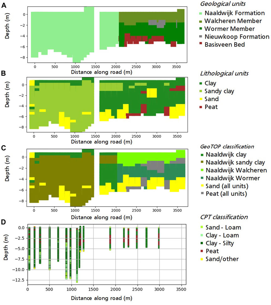
FIGURE 5. This figure is divided into four sections along the road, ranging from A to A′ of Figure 1C. The area around the bridge at ∼1,500 m is not considered in the study and is excluded from the plot. The plot range is up to the depth of the top of the Pleistocene units for all four images. In the top three images (A–C), the depth is derived from the stratigraphical GeoTOP model. In image (D), the depth is based on our own analysis. Image (A) shows the stratigraphical classes from GeoTOP, while image (B) displays the lithological units from GeoTOP. Image (C) illustrates the result of our soil class subdivision, which is based on the stratigraphical and lithological GeoTOP model. Image (D) shows the soil classification for the CPTs along the road sections.

2.1.2 GeoTOP

GeoTOP (TNO-GSN, 2023) is a 3D geological subsurface model with a cell-size of 100 m × 100 m × 0.5 m that schematizes the subsurface of the Netherlands up to a depth of 50 m with respect to NAP. Each cell contains the most probable estimate of lithoclass and lithostratographic unit (classes of soil type) (Stafleu et al., 2011; Van der Meulen et al., 2013). The model is based on ca. 455.000 borehole description from the national subsurface database DINO (TNO-GSN, 2023) and ca. 125.000 borehole logs from Utrecht University.

GeoTOP provides two classifications; one based on lithoclasses (Figure 5B) and one based on lithostratigraphic units (Figure 5A). Lithoclasses subdivide the deposits into their physical character by their sediment grainsize (e.g. sand and clay). Lithotratigraphic classes are based on stratigraphic position of certain units with a certain lithology. This often relates to the age and depositional environment of geological units (e.g. tidal or fluvial, Holocene or Pleistocene).

The GeoTOP lithoclasses were grouped into four categories based on mechanical behavior: peat, clay, sandy clay, and sand/anthropogenic; the latter consisting of non-compressible brought-up construction material, primarily sand. The GeoTOP lithostratigraphic classes within the Holocene sequence of our study area consist of five units (Figure 2); three tidal units: Naaldwijk Formation, Walcheren Member, Wormer Member, and two peats units: Nieuwkoop Formation and Basisveen Bed.

We made the following distinct categories based on lithoclass and lithostratigraphy combinations: sand/anthropogenic, Naaldwijk Formation clay, Naaldwijk Formation sandy-clay, Walcheren Member clay, Wormer Member clay, and the lithoclasses sand and peat (Figure 5C). The lithoclass sand of the different Holocene lithostratigraphic units were grouped together, because they have similar low-compressibility and are expected to show similar behavior. As for peat, we combined both the Nieuwkoop Formation and Basisveen Bed into a single peat category. Note that the lithoclass peat can also be part of the tidal deposit geological units and the lithoclass sand part of the geological units of peat. This applies to a limited number of grid cells at depths larger than 2 m. The effect is therefore expected to be limited.

2.2 Settlement model

To identify the rate and spatial variation of the settlement process in relation to lithoclass and lithostratigraphy, we employed a forward model that quantifies subsidence by settlement using underlying physics. The forward model that we used describes the behavior of the subsurface under loading stress by the road embankment that induces a significant increase in the vertical effective stress causing clay and peat layers to compress.

Calculation of the load of the embankment was based on the average structure of similar road types in the Netherlands. It consists of a 220–250 mm thick layer of asphalt on top of 300 mm granulate and a 500 mm thick sand layer (Crow, 2021). The average densities for each layer were estimated to be respectively 2,500 kg/m³, 1,800 kg/m³ and 1,700 kg/m³, resulting in an average weight of the road embankment of 1.9 * 104 N/m².

We assumed a constant phreatic groundwater level and full saturation of all the layers, thus neglecting changes in vertical effective stress caused by changes in hydrostatic pressure. This assumption is based on the data of TNO-GSN (2023), where nearby groundwater monitoring sites show stable groundwater levels with mere seasonal fluctuations between 10 and 50 cm below the surface. By considering fully saturated conditions, we assumed the road embankment hampered seasonal processes such as swelling and shrinkage of clay and the oxidation of organic material: seasonal effects are known to prevail in free field conditions in the coastal plains of the Netherlands (Fokker et al., 2019), but are negligible when covered by anthropogenic overburden (Koster et al., 2018).

2.2.1 The NEN-Bjerrum settlement model

To determine subsidence caused by loading of the (sub)surface, we employed the NEN-Bjerrum compression model (Bjerrum, 1967; CURCentre for Civil Engineering, 1996; Den Haan et al., 1996; Visschendijk and Trompile, 2009). The NEN-Bjerrum model is commonly used in civil engineering in the Netherlands. The difference between internationally applied Bjerrum and the adjustments made to this for the Netherlands (NEN-Bjerrum) is the addition of the recompression rate factor (RR; Eq. 4) in the NEN-Bjerrum definition. RR is used to express expansion of soft soil when stresses are reduced. The NEN-Bjerrum compression model calculates the total settlement at a particular location by the superposition of settlement mechanisms of the layers influenced by effective-stress increase.

The NEN-Bjerrum model requires to first calculate the vertical effective stress for each soil layer. The total vertical stress ${\sigma }_t$ is equal to the overburden weight per unit area. The stress increase within a single layer i with a thickness of $\delta h_i$, assuming it is fully saturated with water, can be calculated from top to bottom with Eq. 1.

$\Delta {\sigma }_{t,i}=\left(\left(1-\varphi \right){\rho }_{s,i}+\varphi {\rho }_l\right)g\delta h_i(1)$

In which $\varphi$ is the soil porosity, ${\rho }_{s,i}$ the soil density $i$, ${\rho }_l$ the water density, and $g$ the gravitational acceleration.

The vertical effective stress ${\sigma }^{\prime }$ is the difference between the total stress and the water pressure, which can be calculated for each layer according to Eq. 2.

$\Delta {\sigma }_i^{\prime }=\Delta {\sigma }_{t,i}-{\rho }_l\delta h_i=\left(1-\varphi \right)\left({\rho }_{s,i}-{\rho }_l\right)g\delta h_i(2)$

And the total effective stress for each layer is the superposition of the contributions of effective stress of all layers $i$ above layer $n$ is determined with Eq. 3.

${\sigma }^{\prime }={\displaystyle \sum _{i=1}^n}\Delta {\sigma }^{\prime }(3)$

The NEN-Bjerrum model has a rate-type visco-plastic isotache formulation, based on linear strain. The model assumes that a stress larger than the initial effective stress (preconsolidation stress) causes compaction, which is described by three different components:

1. Elastic (reversible) stress at stresses smaller than the preconsolidation stress. This part is proportional to $\log \frac{{\sigma }^{\prime }}{{\sigma }_0}$ , in which RR is the recompression ratio and ${\sigma }_0$ is the virgin effective stress.

2. Primary consolidation (irreversible). This is consolidation that occurs at stresses larger than the preconsolidation stress ${\sigma }_P$, proportional to $RR\log \frac{{\sigma }_p}{{\sigma }_0}+CR\log \frac{{\sigma }^{\prime }}{{\sigma }_P}$ with CR as the compression ratio and ${\sigma }_0<{\sigma }_P<{\sigma }^{\prime }$

3. Secondary consolidation (irreversible), also referred to as creep, is proportional to $C_{\alpha }\log \frac{t}{{\tau }_0}$ where $C_{\alpha }$ is the secondary compaction coefficient and ${\tau }_0$ the reference time.

The NEN-Bjerrum model assumes instantaneous primary consolidation, whilst creep is a time-dependent process. For time-dependent stresses, the contributions are combined in Eq. 4 (Den Haan et al., 1996; Visschedijk and Trompile, 2009; Bakr, 2015):

$\frac{\Delta h}{h_0}=RR\log \frac{{\sigma }^{\prime }}{{\sigma }_0}+C_{\alpha }\log \left(1+{\int }_0^t{\left(\frac{{\sigma }^{\prime }}{{\sigma }_P}\right)}^{\frac{CR-RR}{C_{\alpha }}}\frac{d\tau }{{\tau }_0}\right))(4)$

We determined the preconsolidation stress (${\sigma }_P$) as the product of the original stress (${\sigma }_0$) and the overconsolidation ratio (OCR). The OCR is an indicator of the stiffening of the soil. Generally, the OCR is between 1 and 5 for Holocene layers in the Netherlands (Van Duinen, 2014). The OCR in our area being unknown, we used a value of 2.0. This value represents a relatively virgin soil that has undergone some compaction, in line with the relatively young age of the coastal deposits in the Friesland coastal plain. ${\sigma }_0$ is obtained by the superposition of the effective stresses of each of the soil layers. During the modeling period, the effective stress is given by the ${\sigma }_0$ and the stress induced by the road embankment (${\sigma }_{road}$). Therefore, the differential stress, which represents the additional stress exceeding the preconsolidation stress, is equal to the vertical effective stress caused by the road embankment. To account for the removal of the top layers during road construction, we took an average thickness of half a meter of top layer removal before road construction. We calculated the preconsolidation stress for each layer prior to the removal of the top layers. Since we did not consider the effects of swelling and assumed that the primary compression phase had already occurred, the Eq. 5 is used to calculate the change in layer thickness.

$\frac{\Delta h\left(t\right)}{h_0}=C_{\alpha }\log \frac{t-t_n+{\theta }_{n-1}}{{\tau }_0}(5)$

${\theta }_n={\left(\frac{{\sigma }_n^{\prime }}{{\sigma }_{n+1}^{\prime }}\right)}^{\frac{CR-RR}{C_{\alpha }}}\left({\theta }_{n-1}+t_n-t_{n-1}\right)(6)$

${\theta }_0={\tau }_0{\left(\frac{{\sigma }_0^{\prime }}{{\sigma }_1}\right)}^{\frac{CR-RR}{C_{\alpha }}}(7)$

σ′_n is the vertical effective stress at timestep n and t_n the time at timestep n (indicated by the substrcipt). θ_n is a correction term for the time to account for the stress history and to ensure a smooth transition between subsequent time steps. θ_n is calculated with Eq. 6. At t = 0, θ₀ is calculated according to Eq. 7. The applied stress was taken constant over time. Reference time of t₀ is the construction date of the road embankment. The construction date of the road embankment was ∼18 months prior to the first acquisition date of the satellite. Furthermore, the pre-loading started 36 months prior to the first satellite acquisition. Figure 6 illustrates the concept of instantaneous primary consolidation, and how the secondary part of the compaction influences the relative thickness change measured and modelled over time. Due to the first acquisition date, the process fitted to the measured subsidence in this study is the secondary compaction. Therefore, the parameters estimated in this study are the values of $C_{\alpha }$ for each of the soil types.

FIGURE 6

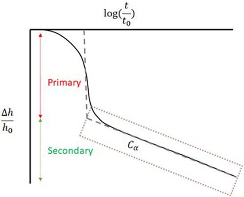
FIGURE 6. This figure shows the effect of primary and secondary compaction to thickness reduction over a logarithmic timescale. The primary compaction according to NEN-Bjerrum acts instantaneously, whilst the secondary compaction or creep increases logarithmic with time. In this study we therefore solely focus on the secondary compaction, as a process that varies with time.

2.3 InSAR displacement estimates

InSAR allows for estimation of small displacements of objects on the surface using radar images (Ferretti et al., 2007). Persistent Scatterer InSAR (PS InSAR) uses multiple satellite images acquired over the same region. Coherent Point Scatterers (PS), having a strong and coherent reflection over a long period, are selected to form a time series of multiple interferograms. The utilized data was sourced from PS-InSAR images from four Sentinel-1 tracks, comprising of two ascending (track 088 and track 015) and two descending tracks (tracks 037 and 110), covering a time period from spring 2015 to spring 2020 with a sampling interval of either 6 or 12 days. For this study we made used of InSAR data that has been processed by a third party, the data was processed by SkyGeo using a PS approach (SkyGeo, 2023).

For our analysis we selected the PS situated on top of the road section but excluded the bridge in the middle of the section. The InSAR estimates represent displacements in the Line-of-Sight (LoS). We considered horizontal movement to be negligible and projected the LoS movement on the vertical direction for each track (e.g., Samieie-Esfahany et al., 2010). The results were used as InSAR derived settlement. To verify whether this was warranted, we checked the similarity of the settlement pattern of all tracks. A difference is expected between the ascending and descending tracks if there is significant horizontal movement, due to their opposite horizontal component.

We analyzed the settlement rate of the InSAR data within a radius of 50 m for each CPT location and per GeoTOP stack of grid cells along the road section in the study area. We compared the behavior of all the satellite tracks to detect outliers. A relative error was derived from the standard deviation from the average rate within the radius, functioning as an estimation of the data quality at each location. This error was further used to scale the absolute error for each data point in the ES-MDA procedure. Figure 7 plots the locations of the GeoTOP grid cell and CPT locations with the linear rate of settlement, as derived from the average timeseries of each location for satellite track 015. The figure shows a different number of locations for the MRM (Figure 7A) and HRD (Figure 7B), which is related to the different number of CPT and GeoTOP grid cells along the road section.

FIGURE 7

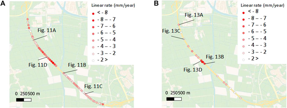
FIGURE 7. (A): The average rate of settlement for each of the GeoTOP grid cells that overlap the road section. (B) The average rate of settlement for each of the CPT location along the road section. The number of locations varies between (A) the average settlement rate of the GeoTOP grid cells and (B), the CPT rates, because the InSAR locations are coupled to the GeoTOP and CPT locations.

2.4 Ensemble smoothing with multiple data assimilation

In order to optimize the parameters of the forward model, we employed a data assimilation approach called ES-MDA (Emerick and Reynolds, 2013; Fokker et al., 2019; Evensen et al., 2022). This method utilizes an ensemble of individual settlement realizations, obtained through Monte Carlo-based selection of the parameters in the forward model, using an average value and standard deviation. The discrepancy between the model estimates and data is calculated, incorporating both settlement and parameter values, for each member of the ensemble. Given the discrepancy, an update function calculates the new ensemble of parameter sets, with a new standard deviation, leading to progressive optimization of the parameters with increasing confidence in each step of the data assimilation.

This principle can also be expressed in the form of an equation, where all the parameters are represented by a vector m and the settlement data into a vector d. The length of m is equivalent to the number of parameters, while the length of d corresponds to the number of data points in space and time. G(m) is the operation of the forward model on the parameters m. The aim is to find m for which G(m) is closest to d. The initial parameters of the study are collected in m₀, and the covariance of the parameters is contained in a matrix C_m, while the covariance of the data is represented by C_d. The least square solution can be obtained by maximizing the Eq. 8 (Tarantola, 2005):

$J=\exp \left(-\frac{1}{2}{\left[\mathit{m}-{\mathit{m}}_{\mathbf{0}}\right]}^T{\mathit{C}}_m^{-1}\left[\mathit{m}-{\mathit{m}}_{\mathbf{0}}\right]-\frac{1}{2}{\left[\mathit{d}-\mathit{G}\left(\mathit{m}\right)\right]}^T{\mathit{C}}_d^{-1}\left[\mathit{d}-\mathit{G}\left(\mathit{m}\right)\right]\right)(8)$

An ensemble of parameter values is collected in a vector M = (m₁, m_2, … , m_Ne) of length N_e, the ensemble size. The values of m are taken from the prior estimate and standard deviation of the parameters. The ensemble of data vectors is created by adding random noise to the original data, again using a Monte Carlo approach, resulting in D = (d₁, d₂, … , d_Ne).

Then, the least square solution of Eq. 8 is solved for the entire ensemble at once, so that GM replaces G(m) in Eq. 8. GM’ is the difference between GM and its average and M′ is the difference between M and its average. The covariance is defined as C_m = M^’M^’T/(N_e-1). And with this the new ensemble of parameters for a subsequent assimilation step can be calculated with one of two equivalent expressions of Eq. 9:

$\widehat{\mathit{M}}=\mathit{M}+{\mathit{M}}^{\prime }{\left[\mathit{G}{\mathit{M}}^{\prime }\right]}^T{\left(\mathit{G}{\mathit{M}}^{\prime }{\left[\mathit{G}{\mathit{M}}^{\prime }\right]}^T+\left(N_e-1\right){\mathit{C}}_d\right)}^{-1}\left(\mathit{D}-\mathit{G}\mathit{M}\right)$

$=\mathit{M}+{\mathit{M}}^{\prime }{\left({\left[\mathit{G}{\mathit{M}}^{\prime }\right]}^T{\mathit{C}}_d^{-1}\mathit{G}{\mathit{M}}^{\prime }+\left(N_e-1\right)\mathbf{I}\right)}^{-1}{\left[\mathit{G}{\mathit{M}}^{\prime }\right]}^T{\mathit{C}}_d^{-1}\left(\mathit{D}-\mathit{G}\mathit{M}\right)(9)$

Depending on the number of parameters versus number of data points one of the two expressions might be more appropriate to use. $\widehat{\mathit{M}}$ is the estimated ensemble of parameters.

The newly estimated parameters and standard deviation that follow from Eq. 9 are used to repeat the optimization. A repetitive application results in a better estimate of the parameters in the case of a non-linear forward model (Emerick and Reynolds, 2013). During the repetitive application of parameter fitting, the data remains the same. To compensate for overfitting towards the multiple application of the same dataset, the covariance of the data is increased for each step of the optimization, with a factor ${\alpha }_i$, to which applies ${\sum }_{i=1}^{nI}\frac{1}{{\alpha }_i}=1$. $nI$ is the number of assimilation steps (Fokker et al., 2019). When ${\alpha }_i$ reduces with a factor q with every assimilation step, the starting value of Eq. 10 must be used:

${\alpha }_0=\frac{1-q^{nI}}{q^{nI-1}-q^{nI}}(10)$

2.4.1 Performance assessment

Different indicators exist to assess the performance of the data assimilation procedure. The performance of the update from the prior to the posterior can be defined by the difference between the estimate and the data, and also by the change in variation in the different parameters between the prior and the posterior. We used three types of assessments: The chi-square error (Fokker et al., 2019), absolute error (AE) and absolute ensemble spread (AES) (Zoccarato et al., 2016).

The chi-square error gives an indication of the difference between the model results and the data, taking into account their covariances. The test function is given in Eq. 11.

${\chi }^2={\left(\widehat{\mathit{G}\mathit{M}}-\mathit{d}\right)}^T{\left({\mathit{C}}_d+{\mathit{C}}_{\widehat{\mathit{G}\mathit{M}}}\right)}^{-1}\left(\widehat{\mathit{G}\mathit{M}}-\mathit{d}\right)(11)$

When the ES-MDA update is good, the average squared mismatch is of the order of the covariance and the outcome should be equal to the number of degrees of freedom, so that: $\frac{{\chi }^2}{Nd}\approx 1$, in which $N_d$ is the number of datapoints.

Both the covariance of the data and of the model results enter the equation to test the overlap between the bandwidth of the data and the bandwidth of the model results. Removing the covariance of the model result may erroneously lead to a too large value when the spread of the results is considerable. Conversely, a very wide distribution of model results can still result in a reasonable quality estimate, as long as it encloses the data. Other measures are also required.

Besides the chi-square error we employ AE and AES to assess the quality of the update of the data (Zoccarato et al., 2016).

The AE indicates the difference between the data and the estimate of the data (Eq. 12).

$AE=\frac{1}{N_e{N}_{dd}}{\mathrm{\Sigma }}_{j=1}^{N_e}{\mathrm{\Sigma }}_{i=1}^{N_{dd}}\left|d{d}_{i.j}-d{d}_{i,true}\right|(12)$

When the actual values of parameters are known it is possible to also quantify the AE for the model parameters. As these are unknown in our study, we only provide an estimate for the data.

The AES (Eq. 13) indicates the variation of the values with respect to the average, i.e., how large the variance in the prediction is.

$AES=\frac{1}{N_e{N}_{dd}}{\mathrm{\Sigma }}_{j=1}^{Ne}{\mathrm{\Sigma }}_{i=1}^{N_{dd}}\left|d{d}_{i,j}-\overline{d{d}_i}\right|(13)$

To provide an assessment of the update from the prior to posterior we calculate for both the AE and AES according to Eq. 14.

$\frac{AE{\left(S\right)}_{posterior}}{AE{\left(S\right)}_{prior}}(14)$

The closer a value to zero, the stronger the constraining force of the ES-MDA. If the constraining force is too strong, the spread of our posterior estimates indicates is lower than realistic, in this case we can speak of ensemble collapse. This makes the results unreliable for uncertainty quantification. In the result section we will use the normalized version for AE and AES as given in Eq. 14, but for simplicity refer to them as AE and AES.

2.4.2 Study specific settings

For this study, the data consisted of a time series of around 150 timesteps. Each InSAR track has its own data count, resulting in 232 timesteps for track 15, 235 for track 88, 246 for track 37 and 243 for track 110. The spatial points were created by an average of all data points located within a radius of 50 m around a CPT location or at the center of a GeoTOP grid cell. The standard deviation of these spatial averages was used to scale the uncertainty around 5 mm for the data vector. Thus, the error varied per location, taking into account the relative variance of the different InSAR timeseries, with the average error set at 5 mm. From these errors per location the covariance matrix for the data was created. Table 1 summarizes the settings and parameters of this study. There are a different number of locations for the HRD and MRM approach. The ensemble size, assimilation steps, q and average error were kept the same for both approaches.

TABLE 1

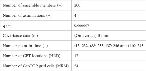
TABLE 1. The settings for the data assimilation procedure.

3 Results

The results are categorized into four sections. The first section showcases the outcomes of the InSAR data examination, where the spatial pattern of settlement is presented graphically. The second section presents a qualitative analysis of the spatial pattern in correlation with the Holocene thickness along the road section. The third section offers the results of a comprehensive analysis of the settlement estimate through data assimilation, utilizing CPT data, which is denoted as the HRD approach. Finally, the fourth section replicates this analysis but uses the MRM approach with the GeoTOP model.

3.1 InSAR data analysis

Figure 8 illustrates the linear settlement rate in mm/year for each InSAR PS estimated from the time series across the length of the road section for all tracks. Additionally, the plot includes the weighted average and standard deviation for the points that fall within a 50 m radius around the CPT locations. The average standard deviation of the ascending tracks (15 and 88) lies around 4 mm and for the descending tracks (110 and 37) it lies around 2.5 mm. The spatial pattern of settlement is found to be similar for all tracks. Because the ascending and descending tracks have opposite horizontal components of the LoS vector, a lack in difference in the behavior of the ascending and descending tracks is in line with our assumption of no horizontal displacements. The rate of settlement increases in segment 1, starting from an average of ∼−2 mm/year to ∼− 9 mm/year around 1,500 m along the road section. In segment 2, the settlement pattern is consistent across all tracks, with an average rate of ∼−2 to −4 mm/year and no clear spatial variance.

FIGURE 8

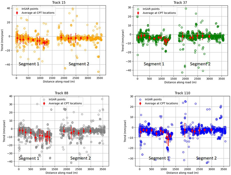
FIGURE 8. The rate of surface displacements obtained from all InSAR tracks along the road is showed, except for the points surrounding the bridge at approximately 1,500 m. The X-axis represents the length along the road from A to A′ in Figure 1B, with the segments indicated in Figure 1C. In addition to the InSAR data, the figure also displays the average rate of settlement for a range of 50 m surrounding the CPT locations, along with the standard deviation of this average. The figure depicts for all tracks an increase in settlement from −4 mm/year to less than −10 mm/year for segment 1, and a stable settlement rate of roughly −4 mm/year for segment 2.

3.2 Qualitative analysis

Figure 9 presents the linear settlement rate from InSAR track 37 overlain on the depth of the base of the Holocene sequence in the area, as derived from the GeoTOP model. When the depth of the base of the Holocene sequences increases—indicating an increase in Holocene thickness, the linear rate of settlement also increases.

FIGURE 9

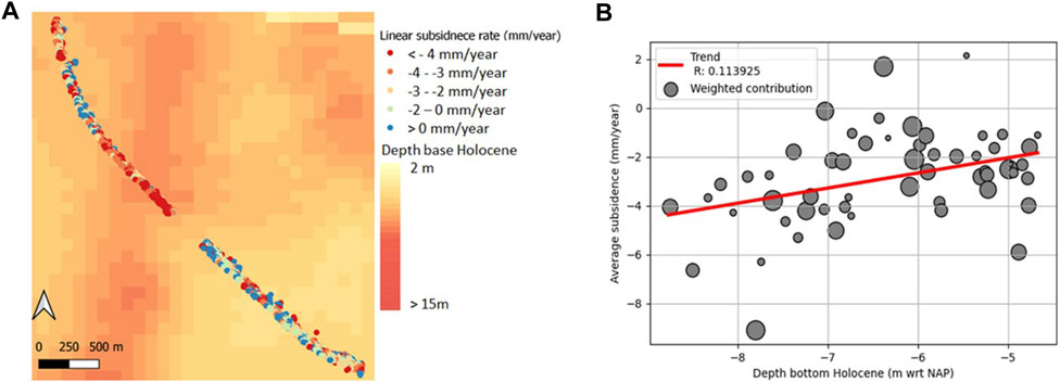
FIGURE 9. (A) Map displaying the depth of the base of the Holocene units according to GeoTOP, with superimposed the settlement rates of InSAR track 37. It is observed that the increase in settlement rates corresponds with an increase in the depth of the base of Holocene units. (B): Plot showing the relationship between the weighted average of InSAR rates, weighted by quality, against the depth of the base of Holocene units at the respective InSAR locations. The plot shows a trend suggesting that larger rates of settlement are associated with greater depth of the base of Holocene units. However, the R² value of 0.11 indicates a weak relationship.

A linear regression analysis is performed to quantify the relationship between the Holocene thickness and the linear settlement rate along the road section. Figure 9B displays a weighted average of the InSAR rate in mm/year versus the Holocene thickness for each GeoTOP grid cell along the road section. The InSAR data points are given weight based on their relative variance within the 50 m radius around each GeoTOP grid cell at the road section. The correlation between the Holocene depth and the linear rate of settlement is weak, with an R² value of 0.11.

3.3 HRD approach (with CPTs)

We subdivided the soil type classes in categories according to Figure 4. The classes peat (2), clay (3) and clay, silty to loam (4) contribute to settlement. Each of the contributing categories was assigned a parameter Cα according to Eq. 5 and Figure 6 for creep compaction. The creep parameters for the different categories act independently. Table 2 shows the resulting parameter estimates. The parameters were given identical starting values of 1.0 ± 0.5 * 10–3, but differentiated vastly after four assimilation steps. The results for the different soil type classes were consistent for the four satellite tracks. The fastest subsiding soil type was peat of class 2, followed by clay of class 3 and clay, silty to loam of class 4. It must however be noted that the spread is large for the peat class and that the number of peat layers is significantly lower than the other classes. The converged values are therefore not very reliable.

TABLE 2

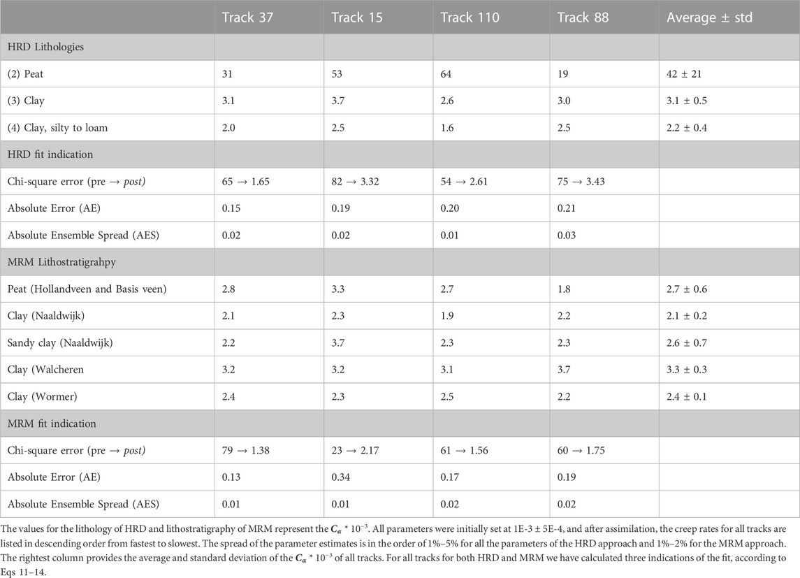
TABLE 2. This table presents the optimized parameters for the HRD and approach with their fit indication.

We plotted the settlement pattern along the road as estimated from the InSAR data and calculated the settlement using the CPT data and the optimized parameters (Figure 10). We observe an increasing rate of settlement along the road section up to −8 mm per year for the CPT data and −12 per year for the InSAR data from 0 to around 1,200 m. The largest increase in subsidence rate is between 750 and 1,200 m from the start of the road section. After 1,200 m rates become stable around −4 mm per year. The transition towards larger subsidence rate between 750 and 1,200 m is bigger for the InSAR data, with a change up to −12 mm per year to −4 mm per year in a few hundred meters.

FIGURE 10

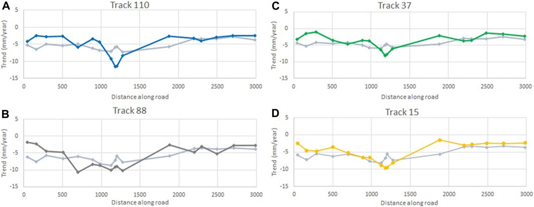
FIGURE 10. Results of the ES-MDA fit with CPT data (HRD). (A–D) correspond to the different satellite tracks. In each plot, the settlement rate is plotted against the distance along the road. The light gray lines give the optimized estimate of settlement rates and the InSAR rates are given with colored lines for each track. The X-axis represents the distance along the road from A to A′ as shown in Figure 1D. The pattern of settlement rate estimated by the CPT data is consistent across all tracks, showing an increase in settlement between ∼750 and ∼1,500 m. After 1,500 m we observe a stable settlement rate of ∼−4 mm/year. The InSAR data shows a similar response for all tracks, although the change in settlement rates between 750 and 1,500 m is sharper.

Figure 11 shows the traces of all the ensemble members for the prior estimate and all assimilation steps for four locations (for locations see Figure 7A). The spread reduces largely, and the fit to the data improves. These improvements are reflected in the changes in the chi-square error, the AE and the AES (Table 2). The AES is around 0.02, indicating a constraining power of the ensemble spread by a factor of fifty. The AE is around 0.20, indicating a large improvement in the absolute error between the prior and posterior estimate with a factor of five. The chi-square errors are all reduced dramatically, but still not one. This, in combination with the AES indicates an ensemble collapse. The constraining power of the data assimilation is similar for all four satellite tracks.

FIGURE 11

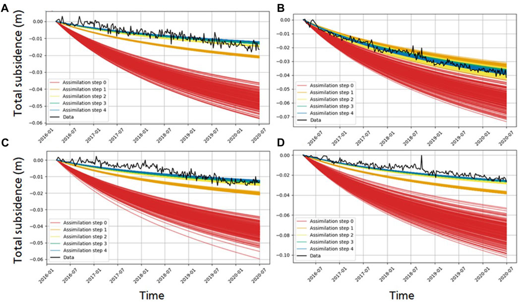
FIGURE 11. Settlement estimates of the time series of four locations for the HRD approach (see Figure 7B for the locations). The black line of the data is the average InSAR timeseries for each location. In four assimilation step, the fit goes from the prior estimate in red (assimilation step 0) to the final estimate in blue (assimilation step 4). We observe that the spread is reduced, and that the final estimate is closer to the data. (A,C) are derived from the results of track 37 and (B,D) from track 15.

3.4 MRM approach (GeoTOP)

Eq. 5 parameter Cα was also optimized for each of the lithostratigraphic classes. Table 2 provides the numeric results. On average, we observe that the clay of the Walcheren Member compacts the fastest, followed bypeat, the sandy clay of the Naaldwijk Formation, and clay of the Wormer Member. The clay of the Naaldwijk Formation shows the slowest creep rates. The differences in parameter values, however, are relatively small.

The settlement rate of the MRM approach and the average InSAR rate are plotted against the road section from A to A′′ (Figure 1D) in Figure 12. Note that the InSAR timeseries of Figure 12 differs from Figure 10, because the points are taken on the locations of the available data (CPT for HRD and GeoTOP for MRM). We observe that the settlement rates are greatest in the section between ∼750 and 1,500 m (−6–7 mm/year for the GeoTOP best estimate and up to −12 mm/year for the InSAR derived rates). The InSAR data shows a more varying pattern and more abrupt changes of settlement rate. Consistently for all tracks, the settlement prediction shows a less sharp increase between ∼750 and 1,500 m than the InSAR pattern. The settlement pattern and rates along the rest of the road section are similar for both the MRM and InSAR data.

FIGURE 12

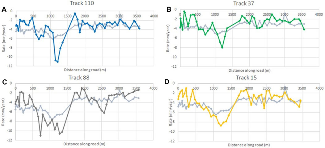
FIGURE 12. Results of the ES-MDA fit with GeoTOP data (MRM). (A–D) correspond to the different satellite tracks. For each track, in light gray the yearly settlement rate derived from the best estimate is provided and the colored lines are derived from the average InSAR timeseries of the locations. The X-axis shows the distance along the road from A to A′, as shown in Figure 1D. The settlement rate pattern estimated by the GeoTOP data is consistent across all tracks, showing an average rate of −4 mm/year settlement, but with increased rates in settlement from ∼750 to 1,500 m up to −6–7 mm/year. The InSAR data shows a similar response for all tracks, although the changes in the settlement are sharper between ∼750 and 1,500 m and can be up to −12 mm/year.

Figure 13 shows the ensemble spread and fit to the data for all the assimilation steps at four selected locations, see Figure 7B. The ensemble spread reduces largely from the prior estimate to the posterior, although at the same time the fit to the data also improves. This is indicated with the quality assessment values of Table 2. The AE and AES of all the tracks are similar. The ensemble spread is strongly constrained, as indicated by the values around 0.02–0.01, which is a constraining factor between 50 and 100. The AE is reduced, with values around 0.2, a five time reduction. The absolute reduction error is indicated with the chi-square error, which lies around the same value for each track except track 15. Track 15 is in the same order, but the difference might be due to the lower number InSAR points around some of the locations, resulting in larger variation in covariance.

FIGURE 13

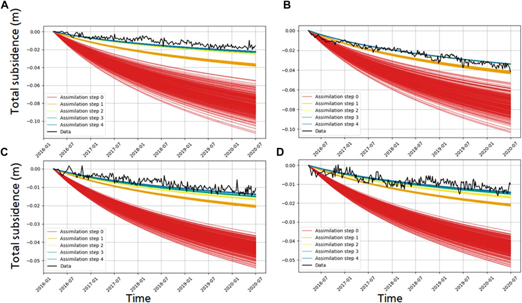
FIGURE 13. Settlement estimates of the time series of four locations for the MRM approach (see Figure 7A for locations) The data is the average InSAR data for each location. In four assimilation steps, the fit goes from the prior estimate (assimilation step 0) to the final estimate (assimilation step 4). The image displays that the spread is reduced, and that the final estimate becomes closer to the data. (A,C) are derived from the results of track 37 and (B,D) from track 15.

4 Discussion

This study demonstrates the added value of combining multiple datasets holding different information on the subsurface for road settlement prediction. The results provide insights into the spatial patterns and characteristics of settlement along the road section. The analysis reveals the relationship between settlement of the road and factors such as the thickness of different Holocene units and the soil types. Furthermore, we have demonstrated that we are able to assess road settlement behavior with non-destructive techniques. To highlight this, we first discuss the results step-by-step, followed by their implications, and end by addressing important points to consider for general application of the developed method.

4.1 InSAR data analysis

The standard deviation of the linear rate of settlement along the road provides an indication of the uncertainty of the estimated displacement rates at the CPT and GeoTOP grid locations. Figure 9 shows that the standard deviation per location (of CPT or midpoint of GeoTOP grid cells) is larger for the two ascending tracks than for the two descending tracks. The main difference between the ascending and descending tracks is the azimuth angle, and therefore the LoS direction. The nature of the reflection points is related to the construction details and orientation of the road infrastructure, such as the guardrail, and can therefore easily be different for the different satellite headings. Another difference between the ascending and descending tracks is the time of passing, in the evening for ascending tracks and in the morning for descending tracks. More turbulence in the air is expected during the evening (Zhao et al., 2023). Such details can result in different variability of the estimates of surface movement derived from different satellite tracks and thus provide an explanation of the difference in behavior we have observed between tracks.

4.2 Coastal plain geology

We found a correlation between thickness of the Holocene coastal sequence and settlement rates, with the highest rates on the road section overlying the deposits of a relative deeply incised tidal channel. A relation between settlement rate and thickness of soft Holocene strata was also empirically established in other areas around the world, for instance in the Mississippi delta (U.S.) (Roberts et al., 1994), Segura River plain (Spain) (Tomás et al., 2010), and the West Pearl River delta (China) (Liu et al., 2023). These areas have in common that differential thickness is often the result of locally occurring incised paleovalley or tidal channel systems. Paleovalleys are elongated incised features that stem from Pleistocene fluvial activity. When sea-levels were low during the Last Glacial Maximum, Pleistocene river systems made broad and deep incisions into underlying deposits (Tanabe et al., 2015; Koster et al., 2017). These incisions provided additional accommodation space for sediments and organics during Early-Holocene relative sea-level rise. The architecture of these paleovalleys consists typically of an elongated feature with orientation more or less perpendicular to the present-day coastline. The infill of its base often consists of clay and peat. Holocene incising tidal channels on the other hand, were often formed during sea-level high stand, when coastal plain formation matured and accommodation space decreased. Their orientation, shape, and size can vary strongly. Their composition often consists of clay and sand (e.g. Vos, 2015).

Correlations between subsurface architecture and settlement rates are valuable when considering the construction of new infrastructure in soft soil areas. Mapping the subsurface will help develop a preliminary understanding of settlement patterns and help prioritize areas for mitigation strategies. However, our analysis indicated a relatively weak correlation between the thickness of the Holocene coastal sequence and the rate of settlement. This is because the thickness of the Holocene sequence is only one factor in the settlement rate. A more elaborate analysis is warranted.

4.3 HRD and MRM approach

The two main differences between the High-Resolution Data and the Medium-Resolution Model approaches are the data density and the subsurface information contained. The HRD approach has sparse data points along the road but a high resolution along the depth of the subsurface; the MRM approach has continuous data but a lower resolution with depth. In addition, the latter data is the result of spatial averaging. The MRM approach contains both soil type and lithostratigraphic information whilst the HRD approach is solely based on soil type.

Both the HRD and MRM approach show the highest discrepancies between model and InSAR data around the channel structure. In the HRD approach the InSAR data is averaged around the sparse CPT locations. The InSAR data smooths the sharp transition on the settlement estimates, whilst the CPT data provides a very local image of the subsurface. The MRM approach on the other hand has a resolution of 100 by 100 m; here the subsurface data smooths the sharp transition of the channel structure, where most distinct changes occur within less than 100 m. Both approaches are unable to catch the small-scale variability of the subsurface properties.

The HRD approach provides a soil type analysis; we observed Holocene soils to behave as expected with finer sediments relating to higher compressibility (Table 2). The MRM approach however shows estimated compaction rates that we would not expect given the lithology (Table 2). The lithostratigraphic interpretation is essential to understand differential settlement along the road. This can be illustrated by the interpretation of the compaction rate estimates of the different lithostratigraphic units. A first indication is the difference in behavior of the Walcheren Member clay and the Wormer Member Clay. The surficial clay beds of the Walcheren Member have the highest compaction rates, the Wormer Member clay shows less compaction. The Wormer Member clay is more overconsolidated, probably because the deposits are buried deeper and were deposited 3,000–5,000 years earlier than the Walcheren Member clay. Hence the Wormer Member clay has undergone thousands additional years of creep. Additionally, Naaldwijk Formation sandy clay shows compaction rates close to those of the Walcheren Member clay beds, which were deposited coeval by the same tidal channel. Based on soil type, sandy clay is expected to compact slower than clay. However, the Naaldwijk Formation channel was formed sub-tidal, therefore the deposits are less ripened by aeration and less over consolidated compared to the supra-tidal clay of the Walcheren Member. The Walcheren Member clay inherently gained substantial stiffness by the ripening process. Another lithostratigraphic unit that does not behave according to lithology is the Naaldwijk Clay member. The Naaldwijk Formation clay member is one of the youngest deposits, however the compaction rates are the lowest for these deposits, this can be explained by the position of these clay beds above the phreatic groundwater level, enhancing the process of ripening and stiffening.

The scale on which the data is available and representative determines the limitations of the settlement estimates. The HRD approach has data on local behavior, whilst the MRM approach employ a more general image of the area. Strong differential settlement is an important cause of damage along the road, making the HRD approach important. With the HRD approach it was recognized that the paleovalley in our study area makes a sharp incise. On the other hand, a continuous estimate of settlement is important. The MRM approach gives a smoothened but continuous image of the subsurface. Hence, a precise analysis of settlement along the road should combine the analysis of both the HRD and MRM approach.

The MRM approach in its specific form with GeoTOP is not internationally accessible, while high-resolution but sparse data with CPT data is widely available. The universal relevance lies in the conceptual framework and insights gained from considering different lithological and lithostratigraphic data, data densities and resolutions and acknowledging data limitations.

4.4 ES-MDA and uncertainty quantification

For both the HRD and the MRM approach we observed that after the four ensemble steps the standard deviation given for each of the estimated parameters is on average less than 5% of the actual value. The spread in calculated surface movement is not enough for the ensemble to cover the measured values, as is indicated by the χ²/N value that is considerably larger than unity and the Absolute Ensemble Spread at one to three percent. For the MRM results the χ²/N values are closer to unity, but the spread in parameter estimates is between 1 and 2 percent. Together with the variation of parameter values from assimilation with the different satellite tracks, this points toward an ensemble collapse. With an ensemble collapse, all the ensemble members have more or less the same value, which suggests a larger certainty for the parameter estimates than is realistic. The phenomenon is more often observed in data assimilation and ES-MDA specific (e.g., Emerick and Reynolds, 2013; Rammay et al., 2022). Trial and error of the initial ensemble spread, and inflation factor did not prevent a collapse. Hence, the results of the actual parameter values should be treated with care, since the standard deviation is most likely underestimated. However, we have an additional means of verification with the variation of the estimated parameters between the satellite tracks for both the HRD and MRM approach. We have used this as an alternative approach to estimate the uncertainty in the parameters, and we arrive at a value around 20% error margin on average.

Our prior estimate consistently overestimated the parameter values, but the final predictions are still in the same order of magnitude. Verberne et al. (2023b) showed that when the initial predictions are outside the range of the actual parameter values, the parameter estimates do not converge. We here have shown that parameter values in the same order of magnitude can converge if the final prediction lies outside the range of the initial prediction. This notion provides some flexibility when estimating the initial parameter values.

4.5 Implications

With the HRD and MRM approach we showed that differential settlement along the road section, as observed consistently with the InSAR data, can be explained by the subsurface composition. We determined how the Holocene coastal sequence translates into settlement along the studied road section. The workflow presented in this study has a broad applicability for infrastructure world wide, as it relies solely on non-destructive datasets that are readily available. If SAR data and subsurface data are available, the approach can be deployed on any given road section and potentially other infrastructures as well, also internationally. Understanding Holocene settlement draws more and more international attention, as it becomes increasingly important as result of sea-level rise, increased droughts and more extensive use of deltaic and coastal areas (Voosen, 2019; Buffardi et al., 2021). Our workflow specifically targets differential subsidence at different scales, an important source of damage, especially in coastal plain areas. One of the key advantages of our workflow is its adaptability to different types of input data. The workflow has been kept simple, meaning no extra InSAR processing steps such as decomposition. Furthermore, the inclusion of different settlement models is seamless, for example enabling the incorporation of factors like primary compaction when using different time ranges. It is important to realize that with data assimilation the observational data and estimates are compared, whilst they often do not have the same spatiotemporal scale. Averaging and interpolation of data is therefore inevitable and can have consequences for the information the data contains.

With regards to the implications for the N31, a difference of more than 5 mm/year can be expected between the fast and slowly subsiding areas. A bridge section is present between these two segments, potentially complicating the damaging effect of the settlement. The potentially most hazardous zone is therefore the area of segment 1 immediately next to the bridge section, on top of the channel structure. This sharpness of this channel structure was made apparent with the HRD and the smoothed and continuous image of the road section. With the MRM approach the smoothed continuous image along the road was determined. The provided explanation to the differential settlement along this road structure can aid in focusing future mitigation and maintenance activities.

5 Conclusion

Our study aimed at better understanding the physics underlying differential settlement of road infrastructure in a soft-soil coastal plain, to identify potential hazard zones. We conclude that modelling settlement along infrastructure requires an understanding on different scales: the behavior of different soil types in high resolution on local scales and lithostratigraphic units on continuous gradual scales. The thickness of Holocene units is an indicator of settlement potential, but the architecture of the Holocene complex is crucial in assessing the differential settlement rates along the road section.

The subsurface is a complex system with multiple levels of variation, which cannot all be taken into account by one source of subsurface data. Therefore, we compared a High Resolution Data (HRD) and Medium Resolution Model (MRM) approach. An analysis of both showed that a sharp transition towards a tidal channel system is the main driver of large differential subsidence. Lithostratigraphic interpretation is paramount, as clayey flat tidal deposits of the Walcheren member, though containing more sand, are subsiding faster than the older and Naaldwijk Formation clay beds. The road section shows differential settlement of over 5 mm/year for an area of less than a kilometer. The total subsidence during the 5 years studied varies between 10 and 50 mm.

Our findings can be used to optimize road maintenance. By using a combination of widely available data types to create a clear image of the settlement pattern, we can identify potential areas of higher risk and improve construction and maintenance practices. Notably, our methodology does not require lab data, making it cheaper and accessible to a wider range of practitioners. In summary, our study highlights the importance of integrating multiple dataset in order to understand the heterogeneities of settlement, which is key to mitigating damage.

Data availability statement

The raw data supporting the conclusion of this article will be made available by the authors, without undue reservation.

Author contributions

MV: Conceptualization, Data curation, Formal Analysis, Investigation, Methodology, Software, Validation, Visualization, Writing–original draft, Writing–review and editing. KK: Data curation, Formal Analysis, Funding acquisition, Project administration, Resources, Supervision, Writing–review and editing. PF: Conceptualization, Formal Analysis, Funding acquisition, Project administration, Resources, Supervision, Writing–review and editing.

Funding

The authors declare financial support was received for the research, authorship, and/or publication of this article. The research presented in this paper is part of the project Living on Soft Soils: subsidence and society (grantnr.: NWA.1160.18.259). This project is funded through the Dutch Research Council (NWO-NWA-ORC), Utrecht University, Wageningen University, Delft University of Technology, Ministry of Infrastructure & Water Management, Ministry of the Interior & Kingdom Relations, Deltares, Wageningen Environmental Research, TNO-Geological Survey of The Netherlands, STOWA, Water Authority: Hoogheemraadschap de Stichtse Rijnlanden, Water Authority: Drents Overijsselse Delta, Province of Utrecht, Province of Zuid-Holland, Municipality of Gouda, Platform Soft Soil, Sweco, Tauw BV, NAM.

Acknowledgments

This study would not have been possible without the effort of Bart Meijninger, who provided insights in how to automatically classify the CPT data. Additionally, Wietske Brouwer and Ramon Hanssen provided help with the analysis of the InSAR data. Willem Dabekaussen provided the GeoTOP model in the right format. Ton Markus aided in a clear visualization of Figure 1. We would like to thank SkyGeo for making the Sentinel-1 data available for this study.

Conflict of interest

The authors declare that the research was conducted in the absence of any commercial or financial relationships that could be construed as a potential conflict of interest.

Publisher’s note

All claims expressed in this article are solely those of the authors and do not necessarily represent those of their affiliated organizations, or those of the publisher, the editors and the reviewers. Any product that may be evaluated in this article, or claim that may be made by its manufacturer, is not guaranteed or endorsed by the publisher.

References

Abidin, H. Z., Andreas, H., Gumilar, I., Fukuda, Y., Pohan, Y. E., and Deguchi, T. (2011). Land subsidence of Jakarta (Indonesia) and its relation with urban development. Nat. Hazards 59 (3), 1753–1771. doi:10.1007/s11069-011-9866-9

CrossRef Full Text | Google Scholar

Bakr, M. (2015). Influence of groundwater management on land subsidence in deltas. Water Resour. Manag. 29 (5), 1541–1555. doi:10.1007/s11269-014-0893-7

CrossRef Full Text | Google Scholar

Bjerrum, L. (1967). Engineering geology of Norwegian normally-consolidated marine clays as related to settlements of buildings. G. eotechnique 17 (2), 83–118. doi:10.1680/geot.1967.17.2.83

CrossRef Full Text | Google Scholar

Bucx, T. H. M., Van Ruiten, C. J. M., Erkens, G., and De Lange, G. (2015). An integrated assessment framework for land subsidence in delta cities. Proc. Int. Assoc. Hydrological Sci. 372 (372), 485–491. doi:10.5194/piahs-372-485-2015

CrossRef Full Text | Google Scholar

Buffardi, C., Barbato, R., Vigliotti, M., Mandolini, A., and Ruberti, D. (2021). The holocene evolution of the volturno coastal plain (northern campania, southern Italy): implications for the understanding of subsidence patterns. Water 13 (19), 2692. doi:10.3390/w13192692

CrossRef Full Text | Google Scholar

Candela, T., and Koster, K. (2022). The many faces of anthropogenic subsidence. Science 376 (6600), 1381–1382. doi:10.1126/science.abn3676

PubMed Abstract | CrossRef Full Text | Google Scholar

Crow, (2021). Wegverbreidingen in cementbeton. BetonInfra, kennisplatform CROW. Available at: https://www.betoninfra.nl/kennisportaal/wegverbredingen-in-cementbeton.

Google Scholar

Cui, X., Zhang, N., Zhang, J., and Gao, Z. (2014). In situ tests simulating traffic-load-induced settlement of alluvial silt subsoil. Soil Dyn. Earthq. Eng. 58, 10–20. doi:10.1016/j.soildyn.2013.11.010

CrossRef Full Text | Google Scholar

CUR, Centre for Civil Engineering (1996). Building on soft soils. London: Routledge, 500.

Google Scholar

Den Haan, E. (1996). A compression model for non-brittle soft clays and peat. Géotechnique 46 (1), 1–16. doi:10.1680/geot.1996.46.1.1

CrossRef Full Text | Google Scholar

Du, Y., He, X., Wu, C., and Wu, W. (2022). Long-term monitoring and analysis of the longitudinal differential settlement of an expressway bridge–subgrade transition section in a loess area. Sci. Rep. 12 (1), 19327–19412. doi:10.1038/s41598-022-23829-y

PubMed Abstract | CrossRef Full Text | Google Scholar

Emerick, A., and Reynolds, A. C. (2013). Ensemble smoother with multiple data assimilation. Comput. Geosci. 55, 3–15. doi:10.1016/j.cageo2012.03.011

CrossRef Full Text | Google Scholar

Evensen, G., Vossepoel, F. C., and Van Leeuwen, P. J. (2022). Data assimilation fundementals, A unified formulation of the state and parameter estimation problem. Berlin: Springer. doi:10.1007/978-3-030-96709-3_1

CrossRef Full Text | Google Scholar

Ferretti, A., Monti-Guarnieri, A., Prati, C., and Rocca, F. (2007). InSAR principles: guidelines for SAR 1029 interferometry processing and interpretation. ESTEC: ESA Publications.

Google Scholar

Fokker, P. A., Gunnink, J., Koster, K., and de Lange, G. (2019). Disentangling and parameterizing shallow sources of subsidence: application to a reclaimed coastal area, flevoland, The Netherlands. J. Geophys. Res. Earth Surf. 124, 1099–1117. doi:10.1029/2018jf004975

CrossRef Full Text | Google Scholar

Fugro Geoservices, B. V. (2015). Geotechnisch onderzoek en funderingsadvies. Fugro Geoservices B.V. Rep. 4009-0271-003.

Google Scholar

Garg, S., Motagh, M., Indu, J., and Karanam, V. (2022). Tracking hidden crisis in India’s capital from space: implications of unsustainable groundwater use. Sci. Rep. 12 (1), 651. doi:10.1038/s41598-021-04193-9

PubMed Abstract | CrossRef Full Text | Google Scholar

Gee, D., Sowter, A., Grebby, S., de Lange, G., Athab, A., and Marsh, S. (2019). National geohazards mapping in Europe: Interferometric analysis of The Netherlands. Eng. Geol. 256, 1–22. doi:10.1016/j.enggeo.2019.02.020

CrossRef Full Text | Google Scholar

Khoshlahjeh Azar, M., Shami, S., Nilfouroushan, F., Salimi, M., Ghayoor Bolorfroshan, M., and Reshadi, M. A. M. (2022). Integrated analysis of Hashtgerd plain deformation, using Sentinel-1 SAR, geological and hydrological data. Sci. Rep. 12 (1), 21522. doi:10.1038/s41598-022-25659-4

PubMed Abstract | CrossRef Full Text | Google Scholar

Koster, K., Erkengs, G., and Zwanenburg, C. (2016). A new soil mechanics approach to quantify and predict land subsidence by peat compression. Geophys. Res. Lett. 43 (20), 792–799. doi:10.1002/2016GL071116

CrossRef Full Text | Google Scholar

Koster, K., Stafleu, J., and Cohen, K. M. (2017). Generic 3D interpolation of Holocene base-level rise and provision of accommodation space, developed for The Netherlands coastal plain and infilled palaeovalleys. Basin Res. 29 (6), 775–797. doi:10.1111/bre.12202

CrossRef Full Text | Google Scholar

Koster, K., Stafleu, J., and Stouthamer, E. (2018). Differential subsidence in the urbanised coastal-deltaic plain of The Netherlands. Neth. J. Geosciences 97 (4), 215–227. doi:10.1017/njg.2018.11

CrossRef Full Text | Google Scholar

Liu, Z., Ng, A. H. M., Wang, H., Chen, J., Du, Z., and Ge, L. (2023). Land subsidence modeling and assessment in the West Pearl River Delta from combined InSAR time series, land use and geological data. Int. J. Appl. Earth Observation Geoinformation 118, 103228. doi:10.1016/j.jag.2023.103228

CrossRef Full Text | Google Scholar

Low, W. W., Wong, K. S., and Lee, J. L. (2019). Cost-influencing risk factors in infrastructure projects on soft soils. Int. J. Constr. Manag. 22, 229–241. doi:10.1080/15623599.2019.1617092

CrossRef Full Text | Google Scholar

Lu, Z., Fang, R., Yao, H., Hu, Z., and Liu, J. (2018). Evaluation and analysis of the traffic load–induced settlement of roads on soft subsoils with low embankments. Int. J. Geomechanics 18 (6), 04018043. doi:10.1061/(asce)gm.1943-5622.0001123

CrossRef Full Text | Google Scholar

Lunne, T., Robertson, P. K., and Powell, J. J. M. (1997). Cone penetration testing in geotechnical practice. New York: Blackie.

Google Scholar

Mahya, M., Kok, S., and van der Lelij, (2021). Economic assessment of subsidence in Semerang and Demak, Indonesia. Deltares – Build. Nat. Indonesia Programme – Secur. Eroding Delta Coastlines. 1220476-002-ZKS-0009.

Google Scholar

Mazzanti, P. (2017). Toward transportation asset management: what is the role of geotechnical monitoring? J. Civ. Struct. Health Monit. 7 (5), 645–656. doi:10.1007/s13349-017-0249-0

CrossRef Full Text | Google Scholar

Meijles, E. W., Kiden, P., Streurman, H.-J., van der Plicht, J., Vos, P. C., Gehrels, W. R., et al. (2018). Holocene relative mean sea-level changes in the Wadden Sea area, northern Netherlands. J. Quat. Sci. 33, 905–923. doi:10.1002/jqs.3068

CrossRef Full Text | Google Scholar

Ngan-Tillard, D., Venmans, A., and Slob, E. (2010). Total engineering geology approach applied to motorway construction and widening in The Netherlands: Part I: a pragmatic approach. Eng. Geol. 114 (3–4), 164–170. doi:10.1016/j.enggeo.2010.04.013

CrossRef Full Text | Google Scholar

Ohenhen, L. O., and Shirzaei, M. (2022). Land subsidence hazard and building collapse risk in the coastal city of Lagos, West Africa. Earth's Future 10 (12), e2022EF003219. doi:10.1029/2022ef003219

CrossRef Full Text | Google Scholar

Peduto, D., Giangreco, C., and Venmans, A. A. M. (2020). Differential settlements affecting transition zones between bridges and road embankments on soft soils: numerical analysis of maintenance scenarios by multi-source monitoring data assimilation. Transp. Geotech. 24, 100369. doi:10.1016/j.trgeo.2020.100369

CrossRef Full Text | Google Scholar

Peduto, D., Huber, M., Speranza, G., Ruijven, J. v., and Cascini, L. (2016). DInSAR data assimilation for settlement prediction: case study of a railway embankment in The Netherlands. Can. Geotechnical J. 54, 502–517. doi:10.1139/cgj-2016-0425

CrossRef Full Text | Google Scholar

Pierik, H. J., Cohen, K. M., Vos, P. C., Van der Spek, A. J. F., and Stouthamer, E. (2017). Late holocene coastal-plain evolution of The Netherlands: the role of natural preconditions in human-induced sea ingressions. Proc. Geologists' Assoc. 128 (2), 180–197. doi:10.1016/j.pgeola.2016.12.002

CrossRef Full Text | Google Scholar

Polcari, M., Moro, M., Romaniello, V., and Stramondo, S. (2019). Anthropogenic subsidence along railway and road infrastructures in Northern Italy highlighted by Cosmo-SkyMed satellite data. J. Appl. Remote Sens. 13 (2), 024515. doi:10.1117/1.JRS.13.024515

CrossRef Full Text | Google Scholar

Python Software Foundation (2023). Python language reference. Retrieved at http://www.python.org.

Google Scholar

Rammay, M. H., Alyaev, S., and Elsheikh, A. H. (2022). Probabilistic model-error assessment of deep learning proxies: an application to real-time inversion of borehole electromagnetic measurements. Geophys. J. Int. 230 (3), 1800–1817. doi:10.1093/gji/ggac147

CrossRef Full Text | Google Scholar

Rijksoverheid, M. (2023). Nota over de toestand van ’s rijks financiën, Ministerie van Financiën. Available at: https://www.rijksoverheid.nl/onderwerpen/prinsjesdag/documenten/begrotingen/2022/09/20/miljoenennota-2023.

Google Scholar

Rijkswaterstaat (2013). De haak om leeuwarden – de nieuwe rijksweg bij leeuwarden. Rijkswaterstaat – Minist. Infrastuct. Milieu, NN0913LV028.

Google Scholar

Roberts, H. H., Bailey, A., and Kuecher, G. J. (1994). Subsidence in the Mississippi River delta--Important influences of valley filling by cyclic deposition, primary consolidation phenomena, and early Diagenesis. Gulf Coast Assoc. Geol. Soc. Trans. 44, Pages 619–629.

Google Scholar

Robertson, P. K. (1990). Soil classification using the cone penetration test. Can. Geotechnical J. 27 (1), 151–158. doi:10.1139/t90-014

CrossRef Full Text | Google Scholar

Robertson, P. K. (2009). Interpretation of cone penetration tests — a unified approach. Can. Geotechnical J. 46 (11), 1337–1355. doi:10.1139/t09-065

CrossRef Full Text | Google Scholar

Samieie-Esfahany, S., Hanssen, R. F., van Thienen-Visser, K., and Muntendam-Bos, A. (2010). “On the effect of horizontal deformation on InSAR subsidence estimates,” in Fringe 2009, proceedings of the workshop held 30 november-4 december 2009 (Frascati, Italy: H. Lacoste. ESA-SP), 677.

Google Scholar

Shi, X., Chen, C., Dai, K., Deng, J., Wen, N., Yin, Y., et al. (2022). Monitoring and predicting the subsidence of dalian jinzhou bay international airport, China by integrating InSAR observation and terzaghi consolidation theory. Remote Sens. 14 (10), 2332. doi:10.3390/rs14102332

CrossRef Full Text | Google Scholar

SkyGeo (2023). SkyGeo Netherlands B.V. Available at: https://skygeo.com/.

Google Scholar

Stafleu, J., Maljers, D., Gunnink, J., Menkovic, A., and Busschers, F. (2011). 3D modelling of the shallow subsurface of Zeeland, The Netherlands. Neth. J. Geosciences 90 (4), 293–310. doi:10.1017/S0016774600000597

CrossRef Full Text | Google Scholar

Tanabe, S., Nakanishi, T., Ishihara, Y., and Nakashima, R. (2015). Millennial-scale stratigraphy of a tide-dominated incised valley during the last 14 kyr: spatial and quantitative reconstruction in the Tokyo Lowland, central Japan. Sedimentology 62 (7), 1837–1872. doi:10.1111/sed.12204

CrossRef Full Text | Google Scholar

Thurkow, A. J. (1992). De friese en de noordhollandse droogmakerijen: een vergelijking. Walburg Pers, TNO-GSN (2023) DINOloket. Available at: https://www.dinoloket.nl/.

Google Scholar

Tomás, R., Herrera, G., Lopez-Sanchez, J. M., Vicente, F., Cuenca, A., and Mallorquí, J. J. (2010). Study of the land subsidence in Orihuela City (SE Spain) using PSI data: distribution, evolution and correlation with conditioning and triggering factors. Eng. Geol. 115 (1-2), 105–121. doi:10.1016/j.enggeo.2010.06.004

CrossRef Full Text | Google Scholar

Törnqvist, T. E., Wallace, D. J., Storms, J. E. A., Wallinga, J., van Dam, R. L., Blaauw, M., et al. (2008). Mississippi Delta subsidence primarily caused by compaction of Holocene strata. Nat. Geosci. 1 (3), 173–176. doi:10.1038/ngeo129

CrossRef Full Text | Google Scholar

Van den Born, G. J., Kragt, F., Henkens, D., Rijken, B., De Lange, G., and Van Bakel, J. (2016). Dalende Bodems, stijgende kosten. Netherlands: Planbureau voor de Leefomgeving.

Google Scholar

Van der Meulen, M. J., Doornenbal, J. C., Gunnink, J. L., Stafleu, J., Schokker, J., Vernes, R. W., et al. (2013). 3D Geology in a 2D country: perspectives for geological surveying in The Netherlands. Neth. J. Geosci. 92, 217–241. doi:10.1017/S0016774600000184

CrossRef Full Text | Google Scholar

Van Duinen, T. A. (2014). Handreiking voor het bepalen van schuifsterkte parameters–WTI 2017 Toetsregels Stabiliteit. Technical Report 1209434-003, Deltares.

Google Scholar

Verberne, M., Koster, K., Candela, T., and Fokker, P. A. (2023b) Disentangling shallow and deep sources of subsidence on a regional scale in The Netherlands. Abstract TISOLS – tenth International Symposium on Land Subsidence

Google Scholar

Verberne, M., Koster, K., Lourens, A., Gunnink, J., Candela, T., and Fokker, P. A. (2023a). Disentangling shallow subsidence sources by data assimilation in a reclaimed urbanized coastal plain, south flevolandpolder, The Netherlands. J. Geophys. Res. Earth Surf. 128. doi:10.1029/2022JF007031

CrossRef Full Text | Google Scholar

Vischedijk, M. A. T., and Trompille, V. (2009) MSettle Version 8.2. Emankment design and soil settlement prediction. Deltares report

Google Scholar

Voosen, P. (2019). Seas are rising faster than believed at many river deltas. Science 363, 441. doi:10.1126/science.363.6426.441

PubMed Abstract | CrossRef Full Text | Google Scholar

Vos, P. (2015). Origin of the Dutch coastal landscape: long-term landscape evolution of The Netherlands during the Holocene, described and visualized in national, regional and local palaeogeographical map series. The Netherlands: Barkhuis.

Google Scholar

Vos, P., and Knol, E. (2015). Holocene landscape reconstruction of the Wadden Sea area between Marsdiep and Weser: explanation of the coastal evolution and visualisation of the landscape development of the northern Netherlands and Niedersachsen in five palaeogeographical maps from 500 BC to present. Neth. J. Geosciences 94 (2), 157–183. doi:10.1017/njg.2015.4

CrossRef Full Text | Google Scholar

Yu, B., Liu, G., Zhang, R., Jia, H., Li, T., Wang, X., et al. (2013a). Monitoring subsidence rates along road network by persistent scatterer SAR interferometry with high-resolution TerraSAR-X imagery. J. Mod. Transp. 21 (4), 236–246. doi:10.1007/s40534-013-0030-y

CrossRef Full Text | Google Scholar

Yu, F., Qi, J., Yao, X., and Liu, Y. (2013b). In-situ monitoring of settlement at different layers under embankments in permafrost regions on the Qinghai–Tibet Plateau. Eng. Geol. 160, 44–53. doi:10.1016/j.enggeo.2013.04.002

CrossRef Full Text | Google Scholar

Zhao, Y., Zuo, X., Li, Y., Guo, S., Bu, J., and Yang, Q. (2023). Evaluation of InSAR tropospheric delay correction methods in a low-latitude alpine canyon region. Remote Sens. 15 (4), 990. doi:10.3390/rs15040990

CrossRef Full Text | Google Scholar

Zoccarato, C., Baù, D., Ferronato, M., Gambolati, G., Alzraiee, A., and Teatini, P. (2016). Data assimilation of surface displacements to improve geomechanical parameters of gas storage reservoirs. J. Geophys. Res. Solid Earth 121 (3), 1441–1461. doi:10.1002/2015jb012090

CrossRef Full Text | Google Scholar