 Runjun Chen1
 Mengfei Yu
 Yuanqin Tao
- 1Hangzhou Urban Infrastructure Construction Management Center, Hangzhou, China
- 2Power China Huadong Engineering Corporation Limited, Hangzhou, China
- 3Zhejiang Huadong Engineering Construction and Management Corporation Limited, Hangzhou, China
- 4College of Civil Engineering, Zhejiang University of Technology, Hangzhou, China
- 5Zhejiang Engineering Research Center of Green Mine Technology and Intelligent Equipment, Hangzhou, China
Accurate prediction of ground surface settlements induced by shield construction is of great significance for ensuring the safety of shield construction. This paper proposes a ground surface settlement prediction method for shield tunneling based on Bayesian updating. The sequential observation data during the advance of excavation is utilized to update the key soil parameters, leading to a more accurate settlement prediction for the subsequent excavation stages. Response surfaces are constructed to replace the finite element model as the forward models for higher computational efficiency. A tunnel excavation project in Hangzhou, China, is selected to illustrate the effectiveness of the proposed method. The shield excavation face passes through four soil layers, and two soil parameters (i.e., Young’s modulus and friction angle) of these soil layers are selected as random variables to be updated. The results show that the soil parameters can be effectively updated based on the observation data at multiple points and various excavation stages. The predictions of ground surface settlements are improved by using the updated soil parameters. The prediction accuracy of the proposed method increases as more stages of observation data are sequentially obtained and incorporated.
1 Introduction
Modern urban development involves the construction of various tunnels, such as subway tunnels, underpass tunnels, highway tunnels, and water pipelines. Shield construction has become one of the most commonly used tunnel construction methods due to its high efficiency and low environmental disturbance. However, shield construction inevitably causes soil disturbance and tunnel deformation, which may result in structural damage such as leakage, tube sheet misalignment, and lining cracks. The soil deformation induced by shield tunneling may damage the surrounding buildings and ecological environment if the ground surface settlement is too large. The ground surface settlement becomes more sensitive especially when the tunnel diameter is large (Xie et al., 2016; Gan et al., 2020). Therefore, in order to ensure the safety of the tunnel and the surrounding environment, it is important to evaluate and predict the ground surface settlement induced by shield tunneling.
Prediction methods for ground surface settlement caused by shield tunneling consist of empirical or semi-empirical methods (Peck, 1969), analytical methods (Sagaseta, 1987; Liu et al., 2018; Litwiniszyn, 2022), numerical simulations (Mazek and Almannaei, 2013; Sharifzadeh et al., 2013; Zhang et al., 2022), and the recently emerged data-driven methods (Lin et al., 2022a; Lin et al., 2022b). Among these methods, numerical simulation has been widely used, as it can simulate the tunneling process under complex geological conditions and provide a comprehensive view of the soil stresses and strains induced by tunnel construction (Komiya et al., 1999; Kasper and Meschke, 2006; Kavvadas et al., 2017). The results of numerical simulations are mainly dependent on the setting of geomechanical parameters of the soil mass (Ou et al., 2013; Tao et al., 2024). Although some geotechnical parameters can be measured from in situ and laboratory tests, it is still challenging to determine the reasonable values of soil parameters (Doherty and Bransby, 2021; Tian et al., 2022; Tao et al., 2023; Huang et al., 2023), due to the limited number of tests, the dubious representativeness of sampling points, and the inevitable disturbance of test samples. Inappropriate soil parameters have a directly adverse impact on numerical simulation outcomes and provide improper construction guidance.
Using in situ monitoring data for updating soil parameters is an effective method to determine appropriate soil parameters at various excavation stages (Arai et al., 1983; Al-Khoury et al., 2001; Feng et al., 2004). Specifically, soil parameters are updated based on the in situ monitoring data from the previous excavation stages and then used to predict the subsequent settlements as the tunneling proceeds. There are various methods of inverse analysis in geotechnical engineering, including deterministic and probabilistic inverse analysis. Deterministic inverse analysis regards geotechnical parameters as a unique set of values and ignores the uncertainty associated with the soil properties. The prediction of soil responses (e.g., ground surface settlement) is also a unique value using the estimated unique set of soil parameters. (Yang et al., 2017). On the contrary, probabilistic inverse analysis can not only identify the soil parameters but also quantify the uncertainty of the soil parameters. Soil parameters are treated as random variables to provide all possible geotechnical responses and their probabilities, which are more in line with actual engineering practice (Gens et al., 1996; Eclaircy-Caudron et al., 2007; Yu et al., 2007; Zhao and Yin, 2009; Hashash et al., 2010). Many inverse analysis methods have been developed based on Bayes’ theorem. For example, Finno and Calvello (2005) presented an inverse analysis framework that effectively assimilates the monitoring data to update the soil parameters for braced excavations. Zhang et al. (2010) used the Markov chain Monte Carlo simulation in conjunction with the response surface method to investigate the slope stability. Tao et al. (2020) proposed an inverse analysis method based on the ensemble Kalman filter for embankment settlement prediction. Bayes’ theorem has been extensively applied in geotechnical engineering to address the uncertainty of geotechnical parameters.
Bayesian methods have also gained attention in tunneling problems. For example, Park and Park (2015) performed a probabilistic inverse analysis to estimate the cohesion and friction angle in a tunneling project. Feng et al. (2019) applied the Bayesian updating to estimate the parameters of an empirical tunnel convergence model based on the convergence measurements. Zhao et al. (2021) integrated the Bayesian method with a multi-output support vector machine-based surrogate model to update the rock mechanical parameters for a circular tunnel. However, these studies only considered the ground surface settlement at a single point. It is possible that the overall settlement curve is different although the settlement of a single point is well captured. Moreover, the differential settlement among adjacent points is more influential to the surrounding infrastructures compared to the settlement at one point. Therefore, it is necessary to predict the ground surface settlement at multiple locations.
This study presents a Bayesian method for an improved prediction of tunneling-induced ground surface settlement using the monitoring data at multiple points and various excavation stages. The soil parameters are identified and updated based on the multi-point monitoring data as the tunneling proceeds. The updated soil parameters are then used to predict the ground surface settlement at the subsequent excavation stages. In order to improve the computational efficiency, response surfaces are constructed to replace the finite element model in the Bayesian updating. A tunnel construction project in Hangzhou is used to show the effectiveness of the proposed method.
2 Methodology
2.1 Bayesian updating
Soil properties exhibit inherent uncertainty as soil is a natural material. Thus, it is challenging to obtain reliable geomechanical parameters. In the numerical calculation of geotechnical engineering, the geomechanical parameters of soil have a direct impact on the calculation results. The soil parameters are treated as unknown random variables x (x = [x1, x2, ., xn], n is the number of soil parameters). Bayesian updating is an effective method to infer the soil parameters from limited monitoring data. The Bayesian formula is written as Equation 1 (Kaipio and Somersalo, 2005):
where p(x) is the prior probability density function (PDF) of the soil parameters x, i.e., the PDF of soil parameters when no observation data is available. The prior PDF can be determined based on engineering experience and previous literature (Cao et al., 2016). L(y|x) is the likelihood function, representing the PDF of the observation data y given the soil parameters x. p(y) is the normalization constant with p(y) = ∫L(y|x)p(x)dx. p(x|y) is the posterior PDF of the soil parameters x, i.e., the PDF of soil parameters after incorporating the observation data.
In geotechnical problems, the analytical solution of the posterior distribution of soil parameters is usually unavailable due to the complexity and nonlinearity of the numerical model. In addition, the unknown parameters are usually multi-dimensional, because soil deformation is affected by multiple soil parameters, such as the friction angle and elastic modulus. For the deformation caused by tunnel excavation, the consideration of layered soil also leads to an increase in the number of soil parameters. Calculating the posterior distribution of each parameter requires sophisticated and high-dimensional integrals that are challenging to implement in practice. Therefore, the MCMC sampling technique is used to approximate the posterior distribution of soil parameters (Qi and Zhou, 2017; Zheng et al., 2019).
In this study, the Metropolis-Hastings (MH) algorithm, which is one of the most commonly used MCMC algorithms in geotechnical engineering (Emerick and Reynolds, 2013; Juang et al., 2013; Qi and Zhou, 2017), is used to generate the posterior samples of soil parameters. The computational steps are as follows.
(1) Determine the first sample value x1 for each random variable, either by random sampling from a prior distribution of the parameters or by taking the mean of the prior distribution directly.
(2) When j = 2, 3, 4, ., N:
a) A candidate value for the jth sample is generated from the proposal distribution q(xp|xj−1). Assume that the proposal distribution q(xp|xj−1) is a multivariate normal distribution with mean xj−1 and covariance s × Cprior, where s is the scaling factor, and Cprior is the covariance matrix of the prior distribution of the soil parameters. The subscript p is an abbreviation for proposal, and the superscript j-1 denotes the j-1st sample.
b) Calculate the probability density ratio r with the formula in Equation 2:
c) Decide whether xp is accepted or not. Draw a random sample u from the uniform distribution U [0,1]. If u ≤ min(r,1), then xj = xp, otherwise xj = xj−1.
d) If j = N, stop MCMC sampling; otherwise, let j = j+1 and repeat steps a)-d).
The MCMC sampling is deemed to have high efficiency if the acceptance rate is between 20% and 40% (Gelman et al., 1995). If the scaling factor s is too large, a large number of samples will be rejected, then the acceptance rate will be too low, and the Markov chain will converge slowly. On the contrary, if the scaling factor s is too small, the proposal samples will move slowly through the parameter space, resulting in a narrow distribution, a high acceptance rate, and low sampling efficiency. In order to attain an effective MCMC sampling, the magnitude of the scaling factor s must be adjusted by trial computations for specific applications.
2.2 Orthogonal design
Orthogonal design is an experimental design method for studying multiple influential factors and multiple levels of these factors. It uses an orthogonal array to arrange and analyze multi-factor experiments for the purpose of obtaining reliable data with a small number of trials. In this paper, an orthogonal design is used to construct a small number of representative sets of soil parameters that are uniformly distributed in the parameter space. These parameter sets are then used as input to obtain the training samples. As a result, the number of numerical simulations required for constructing reliable response surfaces is substantially reduced.
In the orthogonal design method, the parameters considered are called factors. Each factor is assigned with different values within its own permissible value range, the number of values is known as the level of each factor. Under a fixed number of factors, the number of experiments or simulations in the orthogonal design method increases with the number of levels of the factors (Jiang et al., 2018).
Orthogonal designs are usually expressed as La(bc), where L represents the orthogonal table, a represents the number of experiments, b represents the level of each factor, and c represents the number of factors. For example, the meaning of L8(27) is explained as follows: the orthogonal design method designs eight experiments with seven factors (a1, a2, a3, a4, a5, a6, a7), and each factor has two levels (1, 2), as shown in Table 1.

TABLE 1. Orthogonal design table.
The orthogonal design must meet the following three requirements.
(1) For each factor, the occurrence frequency of each level needs to be the same. For example, in Table 1, Level 1 and Level 2 appear four times in each column.
(2) For any two factors, each combination of levels must occur an equal number of times. For example, in Table 1, the combination of levels for factors a1 and a2, namely, (1, 1), (1, 2), (2, 1), and (2, 2), occurs twice each.
(3) The number of trials cannot be less than the square of the number of levels.
2.3 Response surface method
Forward model is a crucial part of updating geotechnical parameters during inverse analysis. In geotechnical engineering, where suitable analytical models are challenging to derive, numerical models are more frequently used to calculate the response of geotechnical structures. However, in general, numerical models are relatively time-consuming to assess the response of geotechnical structures, especially for the MCMC method, which requires 105 to 106 runs of model (Xiao and Cinnella, 2019) and is computationally too expensive. Therefore, the response surface is needed as an alternative forward model (Guo and Dias, 2020; Guo et al., 2022; Tian et al., 2022; Gu et al., 2023). The fundamental principle of response surface method (RSM) is to establish a relationship between the input parameters and the geotechnical response. This is achieved by using a polynomial function, denoted as h(x). In this study, a polynomial function including the constant term, first-order terms, and squared terms is used, which is written as
where h(x) denotes the response surface, x = [x1, x2, … , xn] are the input parameters of the numerical model, n denotes the number of input parameters, and a, bi, ci are the regression coefficients of the polynomial function. The regression coefficients for the response surface method are obtained by least square method. The main steps are as follows.
(1) For each soil parameter, three representative values are selected as input values for the finite model. These three representative values include μ and μ±2σ, where μ represents the mean and σ represents the standard deviation. The mean and standard deviation of each soil parameter are determined by the test data extracted from the geological survey report, existing relevant literature, and the experience of engineers.
(2) The dataset used for developing the response surfaces is generated from numerical model simulations. The orthogonal design in Section 2.2 is adopted to design N sets of input parameters. The corresponding outputs (i.e., ground surface settlements) are calculated through N rounds of numerical simulations.
(3) Based on the dataset, non-linear fitting is performed to determine the regression coefficients of the response surfaces that link the soil parameters and the geotechnical response. It is worth noting that the response surface is different for each excavation stages and monitoring points. It is necessary to construct its own response surface for each monitoring point at each stage. For example, in the real project studied in this paper, there are five excavation steps, and the ground surface settlement needs to be calculated at six monitoring points for each step. Consequently, a total of 5 × 6 = 30 response surfaces need to be constructed.
2.4 Flowchart of the bayesian updating for ground surface settlement
The Bayesian updating flowchart is shown in Figure 1. The method mainly consists of three parts as follows.
(1) Determine the prior distribution of soil parameters. The prior distribution of key soil parameters is obtained based on the geological survey report of the project, previous literature, and engineering experience.
(2) Construct the surrogate model. First, the upper and lower limits of each soil parameter are determined according to the typical value ranges of the soil parameters. N sets of soil parameters is obtained through orthogonal design. These soil parameter sets are then inputted into the finite element model to obtain N output sets of ground surface settlements. Nonlinear fitting is performed to determine the coefficients of response surface for each monitoring point at each excavation stage. The constructed response surfaces is used to replace the finite element model as the forward model in the Bayesian updating.
(3) Perform the Bayesian updating. A sequential updating strategy is adopted as the monitoring data is sequentially recorded with the progress of tunnel excavation. Specifically, the samples generated from the prior distribution of soil parameters are substituted into the constructed surrogate model. The monitoring data of step i is used in the likelihood function. The posterior distribution of soil parameters is derived based on the MCMC sampling. Under the sequential updating framework, the posterior distribution of step i is used as the prior distribution for step i+1. The procedures of data assimilation are repeated until the last excavation stage.
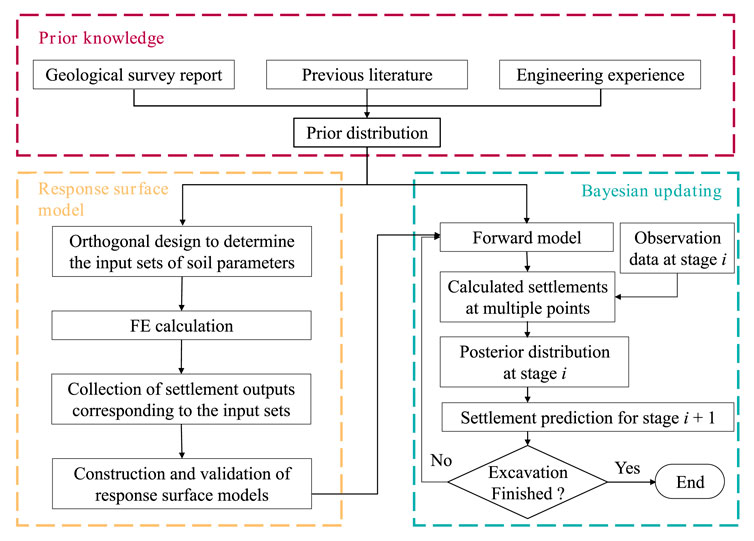
FIGURE 1. Flowchart of the Bayesian updating method for tunneling.
In practical application, once new observation data become available, the soil parameters can be immediately updated in real-time, and the deformation response at the subsequent stages can be rapidly predicted based on the updated soil parameters. It is worth noting that the predicted deformation response is not a single value but a probability distribution.
3 Case study
3.1 Project background
A tunnel project in Hangzhou, China, is used to illustrate the method. The total length of the tunnel is approximately 6.3 km, with an overburden depth of approximately 21 m. The inner and outer diameters of the tunnel are 14.5 m and 13.3 m, respectively. The tunnel consists of 615 rings in total. The section of the 450th ring has a thick soft soil layer in the overlying strata. Therefore, the settlement in this section is likely to be significant, thus it is selected as the prediction target. As shown in Figure 2, the soil profile contains a total of seven layers of soil, and the tunnel mainly crosses the silty clay interspersed with silt, cohesive soil with gravel, strongly weathered mudstone, and moderately weathered mudstone layers. There are five monitoring points at the ground surface within one section, which are at distances of 0 m, 3 m, 7 m, 12 m, 20 m, and 25 m from the tunnel axis, respectively. The ground surface settlement data observed at multiple monitoring points are plotted in Figure 3. Each excavation step is defined as 1 day. This is because the settlement is measured on a daily basis rather than per ring. The date when the tunnel is excavated to the 450th ring is denoted as Step 1, and each of the following 4 days is regarded as an excavation step, e.g., the next day after the excavation of the 450th ring is called Step 2. The number of rings excavated every day is shown in Figure 4.
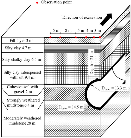
FIGURE 2. Project profile.
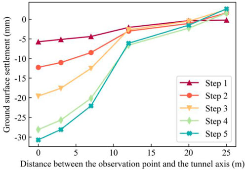
FIGURE 3. Observed data of ground surface settlement at different excavation steps.
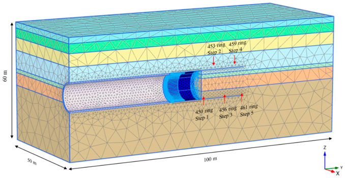
FIGURE 4. Finite element model.
3.2 Numerical model
PLAXIS 3D is used to carry out the numerical simulations. The 3D finite element model of this tunnel project is shown in Figure 4. Only the left half of the tunnel is modeled due to the geometric symmetry of the tunnel, with length = 100 m, width = 50 m, and depth = 60 m.
The tunnel lining segments are simulated using an elastic material with precast C60 concrete. The thickness is 0.6 m, the width is 2 m, the unit weight is 24 kN/m3, the Young’s modulus E is 36 GPa, and the Poisson’s ratio ν is 0.2. The Mohr-Coulomb failure criterion is introduced to simulate the response of the soil. The soil parameters of each soil layer are shown in Table 2. According to the parameter sensitivity study in the existing literature (Miro et al., 2015; Hu and Wang, 2019), the important soil parameters (i.e., Young’s modulus E and friction angle φ) of each soil layer are treated as random variables with coefficients of variation of 0.3 and 0.2 (Phoon and Kulhawy, 1999; Mollon et al., 2009; Qi and Zhou, 2017), respectively. These soil parameters are assumed to follow lognormal distributions to avoid negative values. Other soil parameters (e.g., cohesion c) are considered as constants. An orthogonal design is carried out for 14 random variables to obtain 72 sets of input parameters, as shown in Figure 5. The numbers on the left side of the figure indicate the index of the test, and the number on the top represent a certain soil parameter (e.g., 1 indicates E1, which represents the Young’s modulus for the first soil layer). The numbers in the small squares indicate the level of the parameters, while the values of the levels for a specific parameter are given in the lower table in Figure 5.
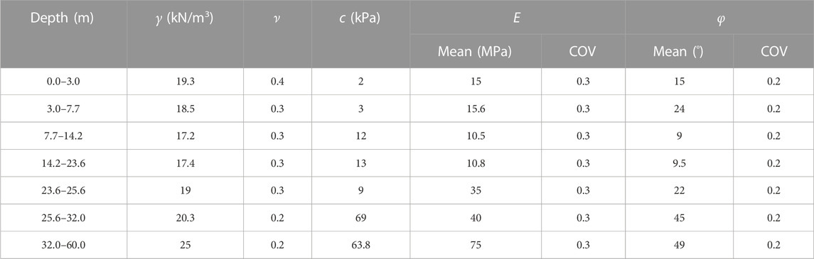
TABLE 2. Soil parameters for seven layers.
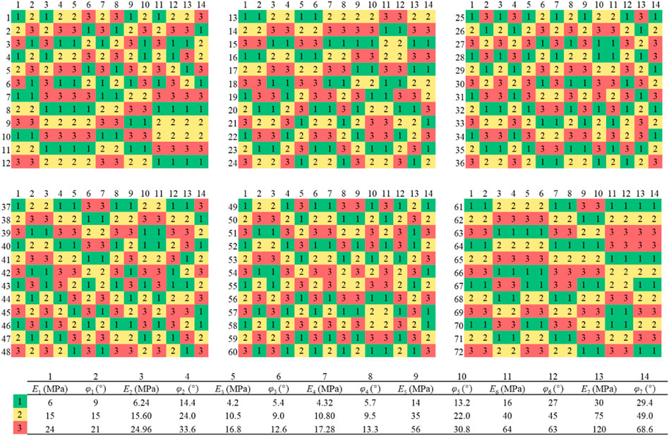
FIGURE 5. Orthogonal design parameter sets.
3.3 Construction of response surfaces
For the tunnel project studied in this paper, a single finite element simulation takes nearly 4 h using a 12th Gen Intel(R) Core (TM) i5-12600 KF (3.70 GHz) computer processor, which is computationally expensive. Therefore, the response surface in Section 2.3 is used instead of the finite element model for the Bayesian updating. The relationship between 14 random variables (the Young’s modulus and friction angle of each soil layer) and ground surface settlement is constructed according to Eq. 3. It is worth noting that the response surface of each monitoring point varies with the steps. Thus, 6 (number of monitoring points) × 5 (number of steps) = 30 response surfaces need to be constructed as described in Section 2.3. The regression coefficients of response surfaces are obtained using the least square method. Figure 6 shows the results of the response surface for the central monitoring point, which is located at the tunnel axis. This response surface is selected for illustration because the settlement near the tunnel axis is usually larger than those at other locations. The settlements calculated from the response surface are generally in good agreement with those directly calculated from the finite element model, as the data points fall around the diagonal line, and the mean absolute error and the coefficient of determination are 3.07 mm and 0.92, respectively. The approximation accuracy may be further improved if more data samples and more complex model forms are used. However, for the tunneling project in this study, the number of data samples is limited because conducting a single 3D finite element simulation is time-consuming. A more complex surrogate model requires more data to estimate the increasing unknown model parameters. In general, the trained response surface is an acceptable approximation of the original finite element model, so it can be used as the forward calculation model in the Bayesian updating.
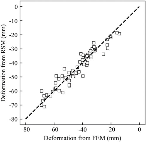
FIGURE 6. Comparison of deformation calculated from the response surface and the finite element model.
4 Results
4.1 Updated soil parameters
In the Bayesian updating, the Young’s modulus and friction angle of the four soil layers traversed by the shield tunneling face are taken as the key parameters to be updated. The Young’s modulus and friction angle of the other three soil layers are taken as constants (i.e., the mean values shown in Table 2). The prior distributions of the key soil parameters are summarized in Table 2. The measurement error is assumed as 5 mm. The length of the Markov chain in the MCMC algorithm is taken as 12,000. After removing the first 2000 samples of the burn-in period, one out of every ten samples is selected as the posterior sample to reduce the correlation between samples (Ching et al., 2021), so the final number of the posterior samples is 1,000.
Figure 7 shows the posterior distributions of soil parameters in each round of Bayesian updating. The soil parameters are updated step by step. Specifically, the posterior distributions of soil parameters obtained from the current step are used as the prior distributions for the next step. As shown in Figure 7, the posterior distribution of each soil parameter is significantly changed as the shield tunneling proceeds and more observations become available. The “short and wide” prior distribution is gradually updated to a “tall and narrow” posterior distribution. The values of the parameters become more concentrated, and the associated uncertainty is significantly reduced. The coefficients of variation of each parameter at each step are summarized in Table 3. It shows that the uncertainty of parameters generally decreases with the increase of incorporated observations. The Young’s modulus is more sensitive than the friction angle, which is consistent with the conclusion from Wang et al. (2022) and Qi and Zhou (2017).
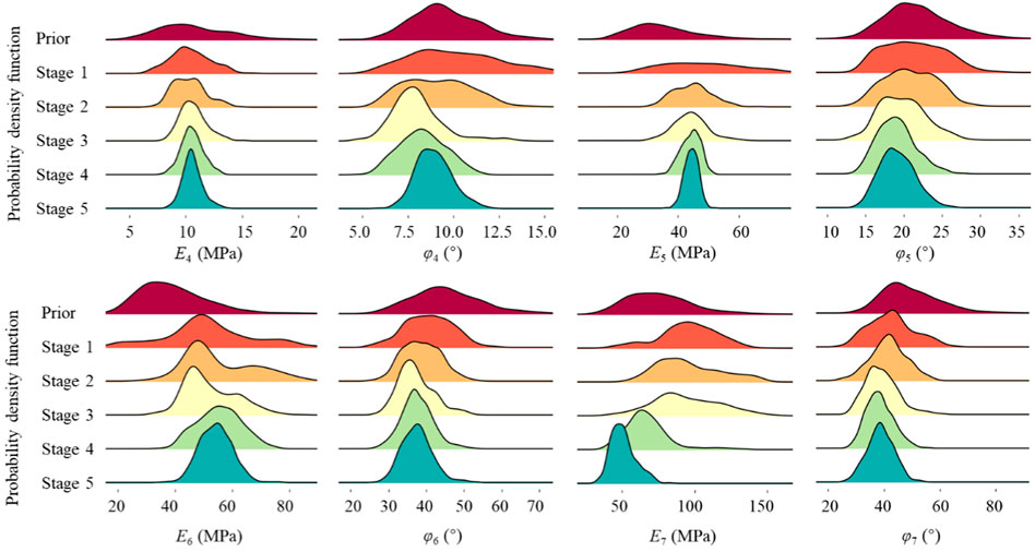
FIGURE 7. Prior and posterior distributions of the soil parameters at various excavation steps.
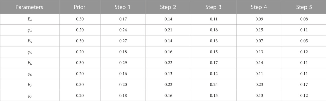
TABLE 3. Coefficients of variation of soil parameters.
4.2 Ground surface settlement prediction
The soil parameters updated based on the available observation data are used to predict the ground surface settlement in the subsequent steps. Figure 8 shows the estimates of ground surface settlement in each step using the posterior distributions of soil parameters obtained from that step. Specifically, as shown in Figure 8A, the soil parameters are updated by incorporating the observation data of Step 1. The ground surface settlement in Step 1 is then estimated using the posterior distributions of soil parameters. It is a back analysis rather than a prediction. The mean and 95% credible interval (CI) are plotted by solid lines and error bars, respectively. The mean settlements calculated from the prior distribution of soil parameters are represented by the dashed lines. It can be seen that the prior distribution of soil parameters significantly overestimates the ground surface settlements and produces a significant bias. This is because the prior distributions of soil parameters are determined based on the geological survey report of the project and the relevant publications. The number of tests provided in the geological survey report is too limited to provide a stable mean value for a soil parameter. The representativeness of the sampling locations is also questionable, and there are inevitable disturbances of test samples. On the contrary, the soil parameters obtained from the back analysis lead to mean settlements close to observations and 95% CIs that generally cover the field observations.
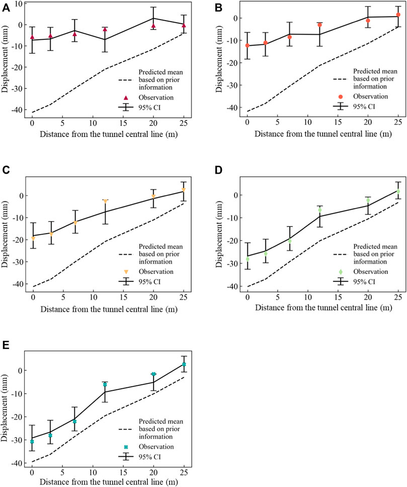
FIGURE 8. Settlement estimate using the posterior distributions of soil parameters from the current step: (A) Estimate for Step 1; (B) Estimate for Step 2; (C) Estimate for Step 3; (D) Estimate for Step 4; (E) Estimate for Step 5.
Figure 9 shows the settlement prediction for the next step using the posterior distributions of soil parameters obtained from the current step. Specifically, as shown in Figure 9A, the prediction of the ground surface settlement in Step 2 is based on the posterior distribution of soil parameters obtained from Step 1. The prediction of ground surface settlement in Figure 9 is generally less accurate compared to that in Figure 8. The difference between the settlement observation and the calculation mean in Figure 9 is larger than that in Figure 8. It is understandable because Figure 8 shows the back analysis results for the current excavation step, while Figure 9 shows the prediction for the next excavation step. In general, as shown in Figure 9, the 95% CIs of predictions can cover most of the observations. In Step 4, there are larger deviations between predictions and observations at the three monitoring points near the tunnel axis, which could be attributed to the separation of the shield tail during that step. The presence of a gap between the tunnel lining segments and the surrounding soil is a result of untimely grouting. However, when the soil parameters are updated by incorporating the observation data of Step 4, the 95% CIs of the predicted surface settlements in Step 5 significantly move towards the field observations. The mean agrees well with the field observations.
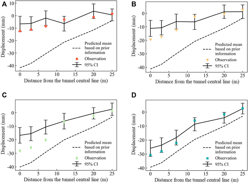
FIGURE 9. Settlement prediction for the next step using the posterior distributions of soil parameters obtained from the current step. (A) Prediction for Step 2; (B) Prediction for Step 3; (C) Prediction for Step 4; (D) Prediction for Step 5.
Figure 10 shows the predicted results of ground surface settlement for Step 5 using the posterior distribution of soil parameters obtained from different steps. The color blocks with different colors indicate the 95% CIs of the ground surface settlement based on the posterior distributions of different steps. The dashed lines indicate the mean settlements. It can be seen that the prediction at the beginning clearly underestimates the ground surface settlement. As the number of available observations increases and more updates are made, the mean settlement gradually approaches the actual observations, and the prediction intervals are slightly narrowed. The root mean square error (RMSE) is used to measure the deviation between the predicted ground surface settlement and the field observations in Step 5. The values of RMSE for each monitoring point at each step are plotted in Figure 11. The prediction results of each monitoring point using the prior distribution deviate significantly from the observations, especially at the monitoring points on the tunnel axis. The deviation between the predictions and the field observations gradually decreases as more monitoring data is incorporated. For example, for the monitoring point on the tunnel axis, the RMSE value is updated from 32.38 mm using the prior distribution to 3.21 mm using the posterior distribution in Step 5. This demonstrates the effectiveness of the proposed method in assimilating observation data to predict ground surface settlement of subsequent steps. In addition, it is worth noting that the influence of new observation data on prediction accuracy gradually diminishes as the tunnel excavation progresses. For instance, at the monitoring point on the tunnel axis, the RMSE between Step 4 and 5 is very small, differing by only 2.56 mm.
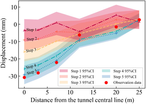
FIGURE 10. Settlement prediction of Step 5 using updated parameters from different steps.
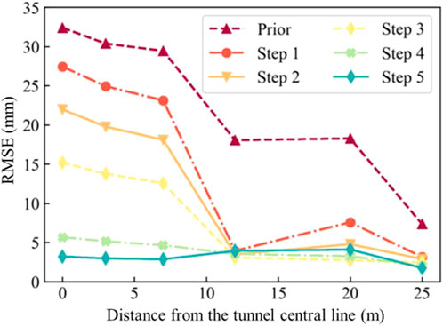
FIGURE 11. RMSE of settlement in Step 5 using updated parameters from different steps.
5 Conclusion
In this study, an effective Bayesian updating method is developed for improving the prediction of ground surface settlement caused by the shield construction. To improve the computational efficiency, response surfaces are employed to replace the finite element model as the forward models in the Bayesian updating framework. Meanwhile, MCMC sampling is used to obtain the posterior distribution of soil parameters. A Bayesian sequential updating method is used to incorporate the observation data at multiple monitoring points during various excavation stages. A tunnel project in Hangzhou, China, is used as an example to illustrate the effectiveness of the proposed method. Based on the results, the following conclusions can be drawn.
(1) This method can effectively identify the soil parameters with quantified uncertainty. During the Bayesian updating of two soil parameters (friction angle and Young’s modulus) of each soil layer, the Young’s modulus is more sensitive to the tunneling-induced ground surface settlements compared to the friction angle.
(2) The accuracy of ground surface settlement prediction is improved as the excavation progresses. As more observation data becomes available, the prediction mean gradually approaches the actual settlement. The 95% prediction interval calculated from the posterior distribution of soil parameters generally covers the actual settlement. In practical projects, once new observations are recorded, they can be incorporated to update the soil parameters for improving the predictions of subsequent settlements.
(3) Response surfaces can replace the finite element model for calculating tunneling-induced settlements. The response surfaces can provide multi-point and multi-stage settlement predictions similar to the finite element model but considerably reduce the computational cost. The efficiency of Bayesian updating is significantly improved, thus facilitating more timely decision-making in engineering.
Data availability statement
The raw data supporting the conclusion of this article will be made available by the authors, without undue reservation.
Author contributions
RC: Conceptualization, Methodology, Writing–original draft, Writing–review and editing. XZ: Conceptualization, Writing–original draft. MY: Methodology, Software, Writing–original draft, Writing–review and editing. JW: Data curation, Software, Writing–original draft. YT: Writing–review and editing, Writing–original draft. FX: Validation, Writing–original draft. YZ: Validation, Writing–original draft.
Funding
The author(s) declare financial support was received for the research, authorship, and/or publication of this article. Author YT would like to thank the National Natural Science Foundation of China (Grant No. 42307218).
Conflict of interest
Authors XZ, JW, and YZ were employed by Power China Huadong Engineering Corporation Limited. Author XZ was employed by Zhejiang Huadong Engineering Construction and Management Corporation limited.
The remaining authors declare that the research was conducted in the absence of any commercial or financial relationships that could be construed as a potential conflict of interest.
Publisher’s note
All claims expressed in this article are solely those of the authors and do not necessarily represent those of their affiliated organizations, or those of the publisher, the editors and the reviewers. Any product that may be evaluated in this article, or claim that may be made by its manufacturer, is not guaranteed or endorsed by the publisher.
References
Al-Khoury, R., Scarpas, A., Kasbergen, C., Blaauwendraad, J., and van Gurp, C. (2001). Forward and inverse models for parameter identification of layered media. Int. J. Geomechanics 1 (4), 441–458. doi:10.1061/(asce)1532-3641(2001)1:4(441)
Arai, K., Ohta, H., and Yasui, T. (1983). Simple optimization techniques for evaluating deformation moduli from field observations. Soils Found. 23 (1), 107–113. doi:10.3208/sandf1972.23.107
Cao, Z., Wang, Y., and Li, D. (2016). Quantification of prior knowledge in geotechnical site characterization. Eng. Geol. 203, 107–116. doi:10.1016/j.enggeo.2015.08.018
Ching, J., Wu, S., and Phoon, K.-K. (2021). Constructing quasi-site-specific multivariate probability distribution using hierarchical Bayesian model. J. Eng. Mech. 147 (10), 04021069. doi:10.1061/(asce)em.1943-7889.0001964
Doherty, J. P., and Bransby, M. F. (2021). A data-driven approach for predicting the time-dependent settlement of embankments on soft soils. Géotechnique 71 (11), 1014–1027. doi:10.1680/jgeot.19.sip.015
Eclaircy-Caudron, S., Dias, D., and Kastner, R. (2007). Assessment of soil parameters met during a tunnel excavation: use of inverse analysis on in situ measurements---Case of Bois de Peu (France). Advances in Measurement and Modeling of Soil Behavior (GSP 173). Denver, CO: ASCE, 1–10.
Emerick, A. A., and Reynolds, A. C. (2013). Investigation of the sampling performance of ensemble-based methods with a simple reservoir model. Comput. Geosci. 17 (2), 325–350. doi:10.1007/s10596-012-9333-z
Feng, X., Jimenez, R., Zeng, P., and Senent, S. (2019). Prediction of time-dependent tunnel convergences using a Bayesian updating approach. Tunn. Undergr. Space Technol. 94, 103118.
Feng, X. T., Zhao, H., and Li, S. (2004). A new displacement back analysis to identify mechanical geo-material parameters based on hybrid intelligent methodology. Int. J. Numer. Anal. Methods Geomechanics 28 (11), 1141–1165. doi:10.1002/nag.381
Finno, R. J., and Calvello, M. (2005). Supported excavations: observational method and inverse modeling. J. geotech. geoenviron. eng. 131 (7), 826–836.
Gan, X., Yu, J., Gong, X., and Zhu, M. (2020). Characteristics and countermeasures of tunnel heave due to large-diameter shield tunneling underneath. J. Perform. Constr. Facil. 34 (1), 04019081. doi:10.1061/(asce)cf.1943-5509.0001362
Gelman, A., Carlin, J. B., Stern, H. S., and Rubin, D. B. (1995). Bayesian data analysis. China: Chapman and Hall/CRC.
Gens, A., Ledesma, A., and Alonso, E. (1996). Estimation of parameters in geotechnical backanalysis—II. Application to a tunnel excavation problem. Comput. Geotechnics 18 (1), 29–46. doi:10.1016/0266-352x(95)00022-3
Gu, X., Wang, L., Ou, Q., and Zhang, W. (2023). Efficient stochastic analysis of unsaturated slopes subjected to various rainfall intensities and patterns. Geosci. Front. 14 (1), 101490. doi:10.1016/j.gsf.2022.101490
Guo, X., and Dias, D. (2020). Kriging based reliability and sensitivity analysis–Application to the stability of an earth dam. Comput. Geotechnics 120, 103411. doi:10.1016/j.compgeo.2019.103411
Guo, X., Dias, D., Carvajal, C., Peyras, L., and Breul, P. (2022). Three-dimensional probabilistic stability analysis of an earth dam using an active learning metamodeling approach. Bull. Eng. Geol. Environ. 81, 40–20. doi:10.1007/s10064-021-02512-y
Hashash, Y. M., Levasseur, S., Osouli, A., Finno, R., and Malecot, Y. (2010). Comparison of two inverse analysis techniques for learning deep excavation response. Comput. geotechnics 37 (3), 323–333. doi:10.1016/j.compgeo.2009.11.005
Huang, X.-W., Guo, J., Li, K.-Q., Wang, Z. Z., and Wang, W. 2023. Predicting the thermal conductivity of unsaturated soils considering wetting behavior: a meso–scale study. Int. J. Heat Mass Transf. 204 123853. doi:10.1016/j.ijheatmasstransfer.2023.123853
Hu, B., and Wang, C. (2019). Ground surface settlement analysis of shield tunneling under spatial variability of multiple geotechnical parameters. Heliyon 5 (9), e02495. doi:10.1016/j.heliyon.2019.e02495
Jiang, Q., Sun, Y., Yi, B., Li, T., and Xiong, F. (2018). Inverse analysis for geomaterial parameter identification using Pareto multiobjective optimization. Int. J. Numer. Anal. Methods Geomechanics 42 (14), 1698–1718. doi:10.1002/nag.2812
Juang, C., Luo, Z., Atamturktur, S., and Huang, H. (2013). Bayesian updating of soil parameters for braced excavations using field observations. J. Geotechnical Geoenvironmental Eng. 139 (3), 395–406. doi:10.1061/(asce)gt.1943-5606.0000782
Kaipio, J. P., and Somersalo, E. (2005). Statistical inversion theory. Stat. Comput. inverse problems, 49–114.
Kasper, T., and Meschke, G. (2006). A numerical study of the effect of soil and grout material properties and cover depth in shield tunnelling. Comput. Geotechnics 33 (4-5), 234–247. doi:10.1016/j.compgeo.2006.04.004
Kavvadas, M., Litsas, D., Vazaios, I., and Fortsakis, P. (2017). Development of a 3D finite element model for shield EPB tunnelling. Tunn. Undergr. Space Technol. 65, 22–34. doi:10.1016/j.tust.2017.02.001
Komiya, K., Soga, K., Akagi, H., Hagiwara, T., and Bolton, M. D. (1999). Finite element modelling of excavation and advancement processes of a shield tunnelling machine. Soils Found. 39 (3), 37–52. doi:10.3208/sandf.39.3_37
Lin, S.-S., Shen, S.-L., and Zhou, A. (2022a). Real-time analysis and prediction of shield cutterhead torque using optimized gated recurrent unit neural network. J. Rock Mech. Geotechnical Eng. 14 (4), 1232–1240. doi:10.1016/j.jrmge.2022.06.006
Lin, S.-S., Zhang, N., Zhou, A., and Shen, S.-L. (2022b). Time-series prediction of shield movement performance during tunneling based on hybrid model. Tunn. Undergr. Space Technol. 119, 104245. doi:10.1016/j.tust.2021.104245
Litwiniszyn, J. (2022). “The theories and model research of movements of ground masses,” in Proceedings of the European congress on ground movement (USA: University of leeds). 209.
Liu, X., Fang, Q., Zhou, Q., and Liu, Y. (2018). Predicting ground settlement due to symmetrical tunneling through an energy conservation method. Symmetry 10 (6), 186. doi:10.3390/sym10060186
Mazek, S., and Almannaei, H. (2013). Finite element model of Cairo metro tunnel-Line 3 performance. Ain Shams Eng. J. 4 (4), 709–716. doi:10.1016/j.asej.2013.04.002
Miro, S., König, M., Hartmann, D., and Schanz, T. (2015). A probabilistic analysis of subsoil parameters uncertainty impacts on tunnel-induced ground movements with a back-analysis study. Comput. Geotechnics 68, 38–53. doi:10.1016/j.compgeo.2015.03.012
Mollon, G., Dias, D., and Soubra, A.-H. (2009). Probabilistic analysis of circular tunnels in homogeneous soil using response surface methodology. J. Geotechnical Geoenvironmental Eng. 135 (9), 1314–1325. doi:10.1061/(asce)gt.1943-5606.0000060
Ou, C.-Y., Hsieh, P.-G., and Lin, Y.-L. (2013). A parametric study of wall deflections in deep excavations with the installation of cross walls. Comput. Geotechnics 50, 55–65. doi:10.1016/j.compgeo.2012.12.009
Park, D., and Park, E.-S. (2015). Inverse parameter fitting of tunnels using a response surface approach. Int. J. Rock Mech. Min. Sci. 77, 11–18. doi:10.1016/j.ijrmms.2015.03.026
Phoon, K.-K., and Kulhawy, F. H. (1999). Characterization of geotechnical variability. Can. geotechnical J. 36 (4), 612–624. doi:10.1139/t99-038
Qi, X.-H., and Zhou, W.-H. (2017). An efficient probabilistic back-analysis method for braced excavations using wall deflection data at multiple points. Comput. Geotechnics 85, 186–198. doi:10.1016/j.compgeo.2016.12.032
Sagaseta, C. (1987). Analysis of undrained soil deformation due to ground loss. Geotechnique 37 (3), 301–320. doi:10.1680/geot.1987.37.3.301
Sharifzadeh, M., Tarifard, A., and Moridi, M. A. (2013). Time-dependent behavior of tunnel lining in weak rock mass based on displacement back analysis method. Tunn. Undergr. Space Technol. 38, 348–356. doi:10.1016/j.tust.2013.07.014
Tao, Y., Phoon, K.-K., Sun, H., and Cai, Y. (2023). Hierarchical Bayesian model for predicting small-strain stiffness of sand. Can. Geotechnical J. doi:10.1139/cgj-2022-0598
Tao, Y., Phoon, K.-K., Sun, H., and Ching, J. (2024). Variance reduction function for a potential inclined slip line in a spatially variable soil. Struct. Saf. 106, 102395. doi:10.1016/j.strusafe.2023.102395
Tao, Y., Sun, H., and Cai, Y. (2020). Predicting soil settlement with quantified uncertainties by using ensemble Kalman filtering. Eng. Geol. 276, 105753. doi:10.1016/j.enggeo.2020.105753
Tian, H.-M., Cao, Z.-J., Li, D.-Q., Du, W., and Zhang, F.-P. (2022). Efficient and flexible Bayesian updating of embankment settlement on soft soils based on different monitoring datasets. Acta Geotech. 17, 1273–1294. doi:10.1007/s11440-021-01378-4
Wang, C., Wang, K., Tang, D., Hu, B., and Kelata, Y. (2022). Spatial random fields-based Bayesian method for calibrating geotechnical parameters with ground surface settlements induced by shield tunneling. Acta Geotech. 17 (4), 1503–1519. doi:10.1007/s11440-021-01407-2
Xiao, H., and Cinnella, P. (2019). Quantification of model uncertainty in RANS simulations: a review. Prog. Aerosp. Sci. 108, 1–31. doi:10.1016/j.paerosci.2018.10.001
Xie, X., Yang, Y., and Ji, M. (2016). Analysis of ground surface settlement induced by the construction of a large-diameter shield-driven tunnel in Shanghai, China. Tunn. Undergr. Space Technol. 51, 120–132. doi:10.1016/j.tust.2015.10.008
Yang, W., Xu, Y., and Wang, J. (2017). Characterising soil property in an area with limited measurement: a Bayesian approach. Georisk Assess. Manag. Risk Eng. Syst. Geohazards 11 (2), 189–196. doi:10.1080/17499518.2016.1208828
Yu, Y., Zhang, B., and Yuan, H. (2007). An intelligent displacement back-analysis method for earth-rockfill dams. Comput. Geotechnics 34 (6), 423–434. doi:10.1016/j.compgeo.2007.03.002
Zhang, L., Zhang, J., Zhang, L., and Tang, W. (2010). Back analysis of slope failure with Markov chain Monte Carlo simulation. Comput. Geotechnics 37 (7-8), 905–912. doi:10.1016/j.compgeo.2010.07.009
Zhang, Z., Liu, W., Huang, X., and Wang, S. (2022). Exploring the three-dimensional response of water storage and sewage tunnel based on 3D finite element modeling. Tunn. Undergr. Space Technol. 120, 104269. doi:10.1016/j.tust.2021.104269
Zhao, H., Chen, B., Li, S., Li, Z., and Zhu, C. (2021). Updating the models and uncertainty of mechanical parameters for rock tunnels using Bayesian inference. Geosci. Front. 12 (5), 101198. doi:10.1016/j.gsf.2021.101198
Zhao, H.-B., and Yin, S. (2009). Geomechanical parameters identification by particle swarm optimization and support vector machine. Appl. Math. Model. 33 (10), 3997–4012. doi:10.1016/j.apm.2009.01.011
Keywords: Bayesian updating, tunnel, response surface method, Markov chain Monte Carlo method, finite element analysis, uncertainty
Citation: Chen R, Zhou X, Yu M, Wu J, Tao Y, Xue F and Zhang Y (2023) Bayesian updating for ground surface settlements of shield tunneling. Front. Earth Sci. 11:1321883. doi: 10.3389/feart.2023.1321883
Received: 15 October 2023; Accepted: 06 December 2023;
Published: 29 December 2023.
Edited by:
Xueyu Geng, University of Warwick, United KingdomReviewed by:
Xiangfeng Guo, South China University of Technology, ChinaHaizuo Zhou, Tianjin University, China
Copyright © 2023 Chen, Zhou, Yu, Wu, Tao, Xue and Zhang. This is an open-access article distributed under the terms of the Creative Commons Attribution License (CC BY). The use, distribution or reproduction in other forums is permitted, provided the original author(s) and the copyright owner(s) are credited and that the original publication in this journal is cited, in accordance with accepted academic practice. No use, distribution or reproduction is permitted which does not comply with these terms.
*Correspondence: Yuanqin Tao, dGFveXVhbnFpbkB6anUuZWR1LmNu