Machine learning analysis and nowcasting of marine fog visibility using FATIMA Grand Banks campaign measurements

Introduction: This study presents the application of machine learning (ML) to evaluate marine fog visibility conditions and nowcasting of visibility based on the FATIMA (Fog and turbulence interactions in the marine atmosphere) campaign observations collected during July 2022 in the North Atlantic in the Grand Banks area and vicinity of Sable Island, northeast of Canada.

Methods: The measurements were collected using instrumentation mounted on the Research Vessel Atlantic Condor. The collected meteorological parameters were: visibility (Vis), precipitation rate, air temperature, relative humidity with respect to water, pressure, wind speed, and direction. Using all variables, the droplet number concentration was used to qualitatively indicate and assess characteristics of the fog using the t-distributed stochastic neighbor embedding projection method (t-SNE), which clustered the data into groups. Following t-SNE analysis, a correlation heatmap was used to select relevant meteorological variables for visibility nowcasting, which were wind speed, relative humidity, and dew point depression. Prior to nowcasting, the input variables were preprocessed to generate additional time-lagged variables using a 120-minute lookback window in order to take advantage of the intrinsic time-varying features of the time series data. Nowcasting of Vis time series for lead times of 30 and 60 minutes was performed using the ML regression methods of support vector regression (SVR), least-squares gradient boosting (LSB), and deep learning at visibility thresholds of Vis < 1 km and < 10 km.

Results: Vis nowcasting at the 60 min lead time was best with LSB and was significantly more skillful than persistence analysis. Specifically, using LSB the overall nowcasts at Vis 1 < km and Vis 10 < km were RMSE = 0.172 km and RMSE = 2.924 km, respectively. The nowcasting skill of SVR for dense fog (Vis ≤ 400 m) was significantly better than persistence at all Vis thresholds and lead times, even when it was less skillful than persistence at predicting high visibility.

Discussion: Thus, ML techniques can significantly improve Vis prediction when either observations or modelbased accurate time-dependent variables are available. The results suggest that there is potential for future ML analysis that focuses on modeling the underlying factors of fog formation.

1 Introduction

Marine fog can form suddenly in marine environments over a range of time and space scales through complex microphysical and dynamic interactions. The intensity of marine fog is expressed in terms of visibility (Vis). An earlier field campaign, called C-FOG (Coastal-Fog), focused on coastal fog and its life cycle along the coastal areas near Nova Scotia, Canada (Gultepe et al., 2021a; Fernando et al., 2021). However, the coastal fog life cycle can be significantly different compared to the marine fog life cycle and can be attributed to the high variability of the fog life cycle with respect to its formation, development, and dissipation across different domains (Gultepe et al., 2007; Gultepe et al., 2016; Koracin and Dorman, 2017). Thus, a specific analysis of marine fog Vis is necessitated.

Marine fog prediction using Numerical Weather Prediction (NWP) models can include large uncertainties over shorter time scales such as less than 6 h (Gultepe et al., 2017). One reason for this is that microphysical parameters cannot be predicted accurately because of the limited knowledge of nucleation processes and microphysical schemes (Seiki et al., 2015; Gultepe et al., 2017). Due to this concern, postprocessing of the NWP model outputs such as air temperature (T_a), dew point temperature (T_d), relative humidity with respect to water (RH_w), wind speed (U_h), and direction (ϴ_dir), precipitation rate (PR), and pressure (P) can be used for Vis predictions (Gultepe et al., 2019). However, for nowcasting applications, many studies are limited because of their large time scales for predictions. For example, predictions based upon ERA5 (fifth generation European Centre for Medium-Range Weather Forecasts (ECMWF) Atmospheric Reanalysis) predictions do not cover shorter time (<1 h) (Yulong et al., 2019) and space scales (<1 km) (Pavolonis et al., 2005; Mecikalski et al., 2007). Space scales based on satellite observations are similarly limited for nowcasting applications because infrared (IR) channels have a resolution of usually 1 km and short-wave infrared (SWIR) channels cannot be used accurately (Pavolonis et al., 2005; Gultepe et al., 2021a) for fog monitoring during the daytime. This suggests that new analysis techniques are needed for nowcasting of fog Vis prediction over time scales less than 6 h.

Studies based on earlier field campaigns used microphysical measurements such as droplet size distribution (DSD) to obtain microphysical parameters (i.e., liquid water content (LWC), droplet number concentration (N_d), and Vis) and develop observational-based Vis parameterizations (Song et al., 2019; Gultepe et al., 2021b; Dimitrova et al., 2021). Although developing Vis parameterizations in this manner is correct, application of these parameterizations to model output data is not straightforward because NWP models cannot accurately predict key microphysical parameters, e.g., LWC, N_d, and RH_w (Bott et al., 1990; Bergot et al., 2005; Zhou et al., 2012; Seiki et al., 2015). Studies have shown that only a 5% error in RH_w or N_d can significantly affect Vis conditions (Kunkel, 1984; Gultepe et al., 2007; Song et al., 2019). Due to these uncertainties in meteorological parameters, new analysis techniques are needed for developing Vis prediction algorithms. An additional study on Vis parameterization, (Gultepe et al., 2006; Gultepe et al., 2017), suggested that a 10%–30% error in N_d can lead to a 100% error in Vis, demonstrating the volatility of N_d-dependent predictions.

The limitations of microphysical parameterizations for NWP models used for Vis prediction suggest that alternate techniques are needed. For example, Yulong et al. (2019) suggested that machine learning (ML) techniques can be used for fog Vis prediction. Such studies mostly used ERA5 reanalysis data or similar archive datasets, which used observations that were hourly, 3-hourly, or even daily (Pelaez-Rodriguez et al., 2023, Yulong et al., 2019). However, fog can form and dissipate in less than a few minutes (Pagowski et al., 2004), thus large/slow-scale model outputs are likely to have biased predictions for smaller/faster-scale events. Another study based on satellite observations, used shortwave (SW) and IR channels on a spatial scale of 1 km to predict fog formation but did not yield insights about Vis (Gultepe et al., 2021b).

In recent years, there has been a focus on predicting the presence of fog, called a binary classification task in the context of ML, given meteorological variables, using either deep learning (Kipfer, 2017; Miao et al., 2020; Kamangir et al., 2021; Liu et al., 2022; Min et al., 2022; Park et al., 2022; Zang et al., 2023) or more standard techniques (Marzban et al., 2007; Boneh et al., 2015; Dutta and Chaudhuri, 2015; Cornejo-Bueno et al., 2017; Wang et al., 2021; Vorndran et al., 2022). Such approaches forego the opportunity for insights regarding the dissipation and formation of fog over time by not predicting fog intensity and, thus, do not lend themselves to characterizing the underlying fog-evolution mechanisms. Furthermore, in the aforementioned studies, the analyzed time resolution was 1 h, presenting no opportunity to even classify rapidly dissipating fog. Predicting the time series of fog visibility was pursued by (Yu et al., 2021), but the time resolution was again limited to 1 h and the lead times were 24 and 48 h, which are not viable operationally. Moreover, there was only one fog event in the prediction interval, which does not provide sufficient information regarding the variability of Vis. Other studies have attempted to predict the times series of visibility, not due to fog, but rather pollution (Zhu et al., 2017; Kim et al., 2022b; 2022a; Ding et al., 2022), and at a coarse time resolution with very few low visibility events (Zhu et al., 2017; Yu et al., 2021).

Although purely deep learning models that inherently account for the autoregressive time series structure have been popular in recent years for various applications such as precipitation nowcasting (Shi et al., 2017; Wang et al., 2017), electricity and traffic load forecasting (Rangapuram et al., 2018), or ride-sharing load forecasting (Laptev et al., 2017; Zhu and Laptev, 2017), such models do not necessarily perform better than non-deep learning techniques (Laptev et al., 2017; Elsayed et al., 2021) unless careful hyperparameter tuning is employed (Laptev et al., 2017). Direct forecasting (Marcellino et al., 2006) with the appropriately lagged variables (Hyndman and Athanasopoulos, 2021) performs on par or even better than the time-dependent deep learning models that are variants of recurrent neural networks (RNNs) (Laptev et al., 2017; Elsayed et al., 2021). Furthermore, deep learning models, particularly RNNs are notoriously difficult to train with data obtained from non-standard settings (Laptev et al., 2017; Elsayed et al., 2021).

In the current study, we used FATIMA (Fog and turbulence interactions in the marine atmosphere) marine fog field campaign’s 1-min observations obtained from various platforms and instruments mounted on the Research Vessel (R/V) Atlantic Condor (Fernando et al., 2022). Measurements were collected over the northeast (NE) of Canada, near Sable Island (SI) and Grand Bank (GB) region of the northwest (NW) Atlantic Ocean (Fernando et al., 2022; Gultepe et al., 2023). Nowcasting of marine fog Vis with the ML regression algorithms of support vector regression (SVR), least-squares gradient boosting (LSB), and deep learning (DL) was performed using lagged versions of these observations. To characterize marine fog with respect to Vis, t-distributed stochastic neighbor embedding (t-SNE) was performed on the whole dataset and projected into 2D space, which organized the data into groups that could be visually assessed with respect to N_d.

2 Materials and methods

The complete data analysis pipeline for nowcasting marine fog Vis time series at lead times of 30 and 60 min, using the 3 ML regression methods of 1) SVR, 2) LSB, and 3) DL at visibility thresholds of Vis <1 km and <10 km is summarized in Figure 1. For analysis, data obtained from 10 intensive observation periods (IOPs) from the FATIMA campaign were used. The collected meteorological variables were preprocessed to create additional time lagged variables, using a lag of 120 min, to take advantage of the latent time-dependent features inherent to the time series data. The following subsections describe the FATIMA field campaign observations, data reduction choices, and 3 ML nowcasting methods.

FIGURE 1

FIGURE 1. Overall preprocessing pipeline used for ML nowcasting Vis.

2.1 FATIMA field campaign and observations

The FATIMA field campaign took place over the northeastern Atlantic Ocean, off the eastern Canada coast (Figure 2) in July of 2022 (Fernando et al., 2022; Gultepe et al., 2023). The R/V Atlantic Condor outfitted with platforms and instruments (Figure 3), collected observations as it sailed from Halifax, NS to Sable Island, NS and the Grand Banks area. The data was collected nearby from Sable Island, NS and the Hibernia oil platform near St. John’s, NL, Canada. Using the Vaisala WXT520 compact meteorological station (Figure 3A) the meteorological parameters of T_a, P, RH_w, and T_d were measured at 1 Hz. From the Vaisala FD70 (Figure 3B), observations related to fog Vis, PR, and type were obtained every 15 s. With the Gill R3A ultrasonic anemometer U_h and ϴ_dir were obtained at 20 Hz. One-minute intervals were applied to aggregate the dataset for analysis. In addition to WXT520 and FD70 measurements, fog microphysics and aerosol measurements were also made, but were not directly used in the analysis, except that the N_d collected from the FM120 was used to qualitatively verify the low Vis conditions. Details on these instruments can be found in Gultepe et al. (2019) and Minder et al. (2023).

FIGURE 2

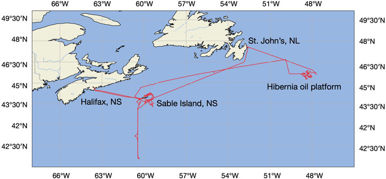
FIGURE 2. The mission path (red colored line) for the R/V Atlantic Condor for collecting detailed microphysics, dynamics and aerosol observations during the FATIMA field campaign. Data was collected near Sable Island, NS and the Hibernia oil platform near St. John’s, NL, Canada.

FIGURE 3

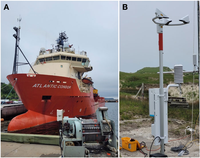
FIGURE 3. (A) The R/V Atlantic Condor, with instruments and platforms used for obtaining measurements. The WXT520 on the upper platform was used to obtain the meteorological observations. (B) FD70 was used to obtain fog visibility and hydrometeor data, such as precipitation rate and amount.

2.2 PR filtering and visibility thresholding

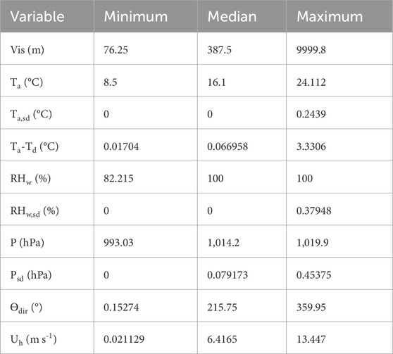
The analyzed measurements for the ML algorithms were fog Vis (km), T_a (°C), ϴ_dir (°), U_h (m s^-1), RH_w (%), and P (hPa). The dew point depression (T_a-Td in °C) and the standard deviations of temperature (T_a,sd), relative humidity (RH_w,sd), and pressure (P_sd) were also computed for each 1-min interval. The six original measured and four computed variables altogether formed 10 parameters (Table 1), which were selected based on literature reviews and physical concepts related to fog formation.

TABLE 1

TABLE 1. Summary statistics of the measurements used for ML analysis.

The dataset was filtered to contain observations with PR < 0.05 mm h⁻¹, due to the fact that rain may confound the prediction of visibility arising from fog, since the impact of rain on visibility can be as large as fog (Gultepe and Milbrandt, 2010). Then, the data was thresholded only to have observations satisfying either, 1) Vis <10 km, to assess how the nowcasting would perform when there is a combination of high and low visibility; and 2) Vis <1 km, to assess how nowcasting would perform when fog is present according to the official definition (American Meteorological Society, 2012). For all variables and analyses, the time resolution of 1 min was enforced to mitigate any further data aggregation.

All 10 variables were initially analyzed using the t-SNE projection method (Maaten and Hinton, 2008). The t-SNE method essentially represents the similarities amongst observations in the high dimensional space in a lower dimensional space (typically 2D or 3D) using the t-distribution, where the fitting procedure is guided by the Kullback-Leibler divergence loss function (Maaten and Hinton, 2008). The t-SNE method, while similar to the multi-dimensional scaling method (Torgerson, 1952), is more effective at exposing nonlinear relationships within the data. The additional benefit of using t-SNE is that it hints at whether clustering methods (e.g., spectral clustering) can successfully find groupings within the data, i.e., “pre-clustering” (Linderman and Steinerberger, 2019). The 2D embeddings obtained from t-SNE were visualized and assessed as to whether the data was organized or grouped in any meaningful way related to N_d.

2.3 Relevant variable selection

To determine which variables would be the most relevant for visibility nowcasting, all 10 variables (Table 1) in the thresholded dataset at Vis <10 km were used for a pairwise correlation analysis and visualized as a heatmap. Only the variables U_h, RH_w, T_a-T_d, were selected because they all had a statistically significant correlation (p < 0.001) and a moderate magnitude of correlation (r > 0.30) with Vis (Ratner, 2009). Additionally, the variable choices are viable in a meteorological context, e.g., it is expected that the RH_w is negatively correlated with Vis since decreasing RH_w indicates the removal/dissipation of fog droplets (Gultepe et al., 2019). RH_w,sd had a moderately positive correlation with Vis, but was not included in nowcasting models because it seemed to capture the same correlation information as RH_w, and using fewer variables would make the ML regression models more parsimonious. Similarly, U_h (advecting moisture and warm air over cold ocean surface) and T_a-T_d are also good indicators of fog formation because T_a-T_d is strongly related to RH_w which is a function of both T_a and T_d. Note that wind direction is not included in the ML nowcasting because the correlation with Vis was low (r = 0.05).

2.4 Lagged features and train-test split

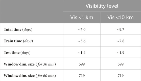
To effectively use ML regression models with time series data for forecasting or nowcasting, the data itself must be transformed to reflect the autoregressive structure of the time series. One of the most effective strategies is to create lagged versions of the input and output variables (Figure 4) and use a regression model to directly predict the desired time step (Hyndman and Athanasopoulos, 2021). In this study, to predict Vis at the 30 and 60 min lead times, 120 min of lag was used for each of U_h, RH_w, T_a-T_d, and Vis. The simple heuristic that the time lag of variables should be twice as long as the longest lead time was used, thus a lag of 120 min was chosen. The principle here is that the regression model should have a sufficiently large lookback window to determine which elements of the lapsed data are relevant for prediction.

FIGURE 4

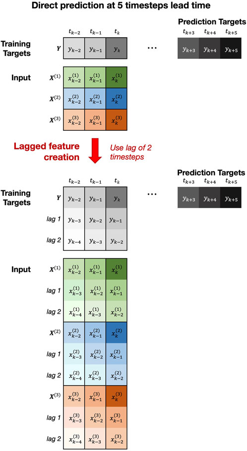
FIGURE 4. Shows an example of how time series data can be restructured for use in ML regression models for direct forecasting. The example shown uses a lag of 2 timesteps to predict 5 timesteps into the future.

The total lookback window size for each variable is $w=lag+leadtime–1$. All 3 ML regression models used in this study implement $L$₂ regularization, which reduces the effect of irrelevant variables. Finally, the data were split into training and testing sets at both visibility levels using the common split of 80% train and 20% test (Hastie et al., 2009). A summary of each visibility dataset is given in Table 2. Figure 5 shows the train and test split for the Vis <10 km data at the 60 min lead time.

TABLE 2

TABLE 2. Summary of datasets used for nowcasting for Vis <1 km and Vis <10 km.

FIGURE 5

FIGURE 5. The train and test split for the time series of the Vis <10 km data at the 60 min lead time is shown.

2.5 Nowcasting with ML regression

Three types of ML regression models, with increasing levels of model flexibility/parameters (Hastie et al., 2009), were employed to demonstrate the effectiveness of direct nowcasting/forecasting (Elsayed et al., 2021; Hyndman and Athanasopoulos, 2021). The hyperparameters (i.e., regularization level, # of training phases, etc.) used in all three models were chosen based on values that are commonly known to be effective in a high-dimensional setting.

Of the three models used, the least complex method is considered to be SVR. It maps input training feature vectors into a higher dimensional space, in which a linearly separating hyperplane that minimizes the residuals of the data points beyond the margin of the hyperplane is fitted (Smola and Schölkopf, 2004; Hastie et al., 2009; Ho and Lin, 2012). The margin parameter in SVR is similar to that of support vector machines, except that it is adapted for regression rather than classification (Hastie et al., 2009). When the dimensionality of the input data is high, as in our case with either 599 or 719 dimensions, using a linear kernel is very efficient and achieves high accuracy despite not using a complex nonlinear kernel, such as a radial basis function (Fan et al., 2008; Hsu et al., 2021). The SVR is implemented with a high amount L₂ regularization with $\lambda$ = 0.0001 to account for the high dimensionality of the input data.

Gradient boosting using the least squares loss function (LSB) was the second implemented regression model due to its popularity and ability to achieve a high level of performance for many tasks, particularly for visibility classification and regression (Yu et al., 2021; Kim et al., 2022a; 2022b; Ding et al., 2022; Vorndran et al., 2022). LSB successively fits many weaker regression trees on the residual error (Hastie et al., 2009). The learning rate (the L₂ regularization parameter in boosting) was set to 0.1, the number of learning cycles was 2000, and the weak learner used was a tree.

The most complex model in terms of the parameter space was the DL regression, composed of multiple stacked fully-connected feedforward neural network layers, i.e., a multilayered perceptron (MLP). The hyperparameter setup of the DL model was: 1) loss function as the mean absolute error (MAE); 2) batch normalization applied before the activation layer; 3) activation function of all intermediate hidden layers set to ReLU (Nair and Hinton, 2010); 4) L₂ weight regularization at $\lambda$ = 0.0001; 5) number of epochs = 40; 6) mini-batch size = 64; 7) ADAM optimizer (Kingma and Ba, 2014); and 8) learning rate of 0.001. The above choice of hyperparameters of the DL model was inspired by (Jha et al., 2019), which demonstrated the key aspects of effective regression using deep neural networks. The hidden layer dimensions of the DL network at the 30 min and 60 min lead times were [256, 128, 64, 32] and [256, 256, 128, 64, 32], respectively. In each model, the final layer is an output node with a dimension 1, which is the regression output at the relevant lead time.

For all 3 ML regression methods, L₂ regularization was used. This is similar to performing ridge regression, which has an additional L₂ regularization term ($\lambda {\sum }_j{w}_j^2$) in the loss function of a linear regression model. The L₂ term in ridge regression and aforementioned ML methods mitigates model weights from dominating each other by constraining the magnitude of the weights, by scaling them using the $\lambda$ parameter (Hastie et al., 2009). Furthermore, to implement the ML regression models effectively, normalization of data is necessary due to the different scales of the variables. Prior to all regression analyses, z-score normalization was applied to both train and test datasets. However, a critical detail of this procedure is to apply the mean and standard deviation from the training dataset to the test dataset, rather than compute the mean and standard deviation separately (Coates et al., 2011). This is commonly overlooked in many implementations and leads to poor model performance due to the fact that the test data is not in the same feature space as the training data (Coates et al., 2011).

2.6 Nowcasting performance evaluation

Root mean squared error (RMSE) was used to assess the nowcasting performance across all 3 ML models for both Vis thresholds (Vis <1 km and <10 km) and lead times (30 and 60 min), which is calculated as below,

$\text{RMSE}=\sqrt{{\sum }_n^1\frac{{\left(\widehat{\text{Vis}}\left(t\right)-\text{Vis}\left(t\right)\right)}^2}{n}}(1)$

The RMSE was used in three different settings: 1) overall RMSE, 2) RMSE for Vis ≤400 m, and 3) RMSE for Vis >400 m. The RMSE of Vis ≤400 m is of particular interest due to the fact it is generally considered the threshold for dense fog, which can impede maritime activities and military operations (Kelsey, 2023; Yang et al., 2010; Mack et al., 1983). Thus, for each nowcasting case, three RMSE values are reported. For the overall RMSE of the nowcasting at the Vis <10 km threshold, the RMSE was weighted proportionally to the number of timesteps that were Vis ≤400, to account for the fact that accurately predicting dense fog is more critical. For the overall RMSE of the nowcasting at the Vis <1 km threshold, such an adjustment was not made since the majority of the timesteps were Vis ≤400.

To further assess the validity of the nowcasts, naive prediction (Hyndman and Athanasopoulos, 2021) of the Vis time series was performed using two types of persistence. The first type of persistence nowcast, referred to as Per, was calculated as,

$\text{Vis}\left(t+h\right)=\text{Vis}\left(t\right)(2)$

where h is either 30 min or 60 min (Hyndman and Athanasopoulos, 2021). The second type of persistence nowcast, referred to as PerW, was computed as,

$\text{Vis}\left(t+h\right)=\left(\text{Vis}\left(t-w\right)+\dots +\text{Vis}\left(t\right)\right)/w(3)$

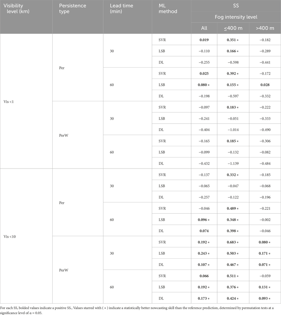
which is the mean of the Vis in the lookback window w (Hyndman and Athanasopoulos, 2021). The RMSE calculations of both Per and PerW follow the same aforementioned structure as the ML regressions. Using the persistence RMSE calculations as the reference RMSE (RMSE_ref) in Eq. 4, the skill scores (SS) were calculated as,

$\text{SS}=1-\frac{{\text{RMSE}}_{\text{nowcast}}}{{\text{RMSE}}_{\text{ref}}}(4)$

where an SS of 1 indicates perfect nowcast with no error, an SS of 0 indicates the same performance as persistence, and a negative SS indicates worse than persistence (Wilks, 2006). Thus, for each nowcasting setting, two sets of SS were obtained, SS using Per (SS_Per) and SS using PerW (SS_PerW). To determine whether a positive SS indicated significantly better nowcasting than persistence, one-sided permutation tests were performed between the squared residual errors of the ML and persistence nowcasts using 10,000 permutations, at a significance level of α = 0.05 (Good, 2013). Specifically, the null hypothesis ($H_0$) assumes that there is no difference between the means of the squared residual errors of the ML and persistence nowcasts, whereas the alternate hypothesis ($H_A$) assumes that the actual ML nowcast has a smaller mean squared residual error than the persistence nowcast. The null distribution was constructed by obtaining differences in means from randomly permuted and grouped sets of squared residual errors from the ML and persistence nowcasts (Storch and Zwiers, 2003; Wilks, 2006).

All methods were implemented using MATLAB 2022b on a system with Ubuntu 20.04 LTS Linux OS, Intel Core i9-10980XE 3.0 GHz 18-Core Processor, 256 GB RAM, and dual NVIDIA Quadro RTX 5000 GPUs.

3 Results

In Figure 6, the clustering of the Vis observations using the t-SNE plot demonstrates that at the lower levels of Vis (Vis ≤400 m and 400 < Vis ≤1,000 m), there may be two physical discriminations of Vis. Based on the definition of fog microphysical parameters, the accumulation of the data points in the two regions at Vis ≤1,000 m is likely due to fog microphysical conditions. Gultepe et al. (2007) showed that Vis is the function of both LWC and N_d, and the same Vis can be obtained by changing droplet spectral characteristics, such as the variance and spectral gaps, both of which are critical conditions that affect nowcasting of the Vis parameter. However, the clusters in the t-SNE plot were obtained without using either of the values in the analyses, which suggests that LWC and N_d may be acting as latent processes in the observations used in the current study.

FIGURE 6

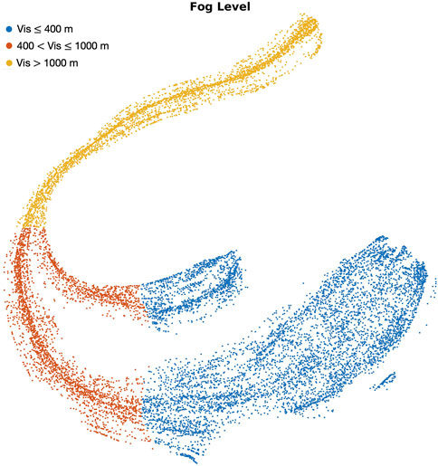
FIGURE 6. The t-SNE plot of the observed Vis. The plotted clusters show that despite having the same level of Vis, the observations may be reflecting the underlying distribution of the N_d and LWC values although they were not used in any analysis for this study.

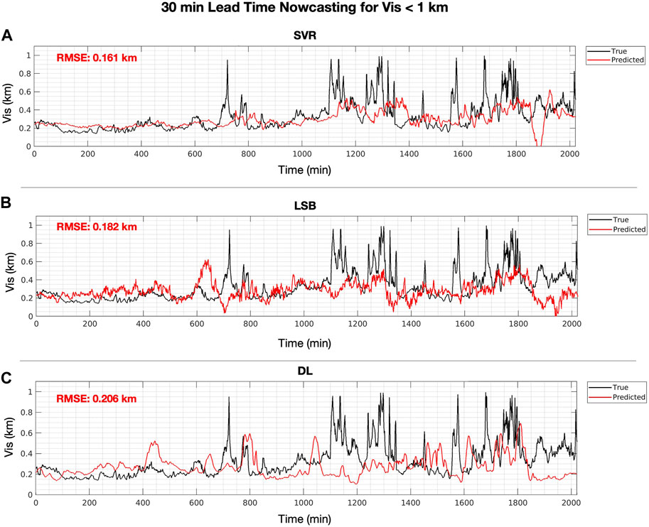
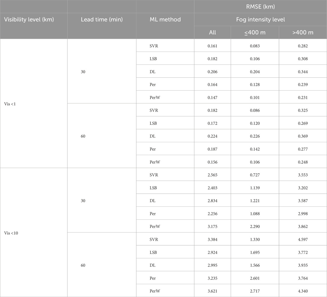
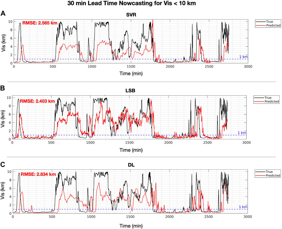
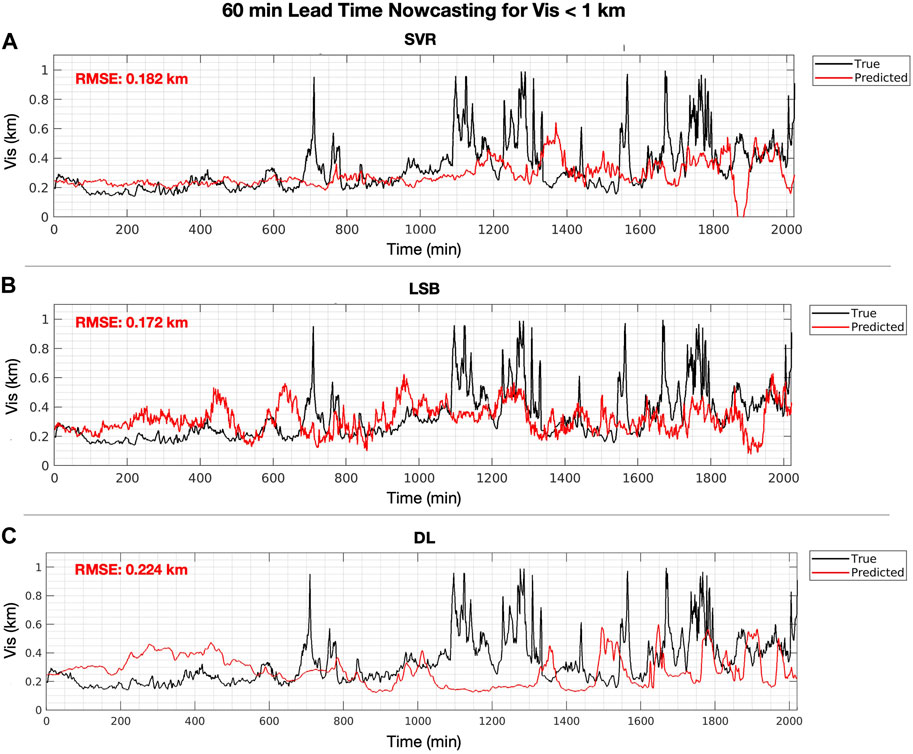
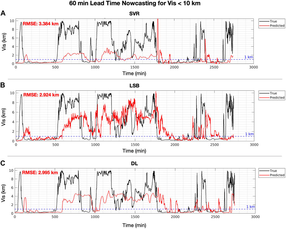
Using the selected variables of U_h, RH_w, and T_a-T_d, which were among the highest correlated with Vis as shown in the correlation heatmap (Figure 7), nowcasting with SVR, LSB, and DL regression was performed for four different cases: 1) Case 1: lead time of 30 min, Vis <1 km; 2) Case 2: lead time of 30 min, Vis <10 km; 3) Case 3: lead time of 60 min, Vis <1 km; and 4) Case 4: lead time of 60 min, Vis <10 km. The RMSE and SS of the nowcasts are shown in Tables 3, 4, respectively. In Figures 8–11, the time series plots of the Vis nowcasts against the observed Vis are shown. The Supplemental Material contains the nowcast plots for both Per and PerW methods in all four cases.

FIGURE 7

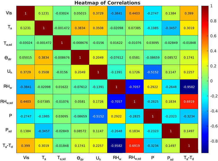
FIGURE 7. Heat map of the meteorological parameters used in the ML analysis. When r > 0.3, variables are considered to be significant and used in the analysis. The variables U_h, RH_w, T_a-T_d were selected for analysis as they had statistically significant correlation (p < 0.001) and a moderate magnitude of correlation (r > 0.30) with Vis.

For Case 1, at the 30 min lead time and Vis <1 km (Figure 8), only the SVR (SS_Per = 0.019) method with an RMSE of 0.161 km had a better overall nowcast than Per (RMSE = 0.164 km), but according to the permutation test it was not significantly better. The other two methods of LSB and DL performed worse than Per. Yet, the nowcasts of both SVR (SS_Per = 0.351) and LSB (SS_Per = 0.166) for dense fog were both significantly better than Per, but none of the SS_Per for the three methods were positive for non-dense fog. This indicates that these 2 ML models are able to track dense fog, but have difficulty in tracking less dense fog for Case 1. None of the SS_PerW (Table 4) values for the overall RMSE (Table 3) nowcasts exceeded the PerW reference nowcasting. This is expected since the PerW uses the mean of the lookback window and the majority (73.8%) of the Vis values in the testing period are ≤400 m for many consecutive time steps. As such, it is rather difficult to perform better than PerW in this case due limited variation of the Vis. Yet SVR (SS_PerW = 0.183) was able to significantly better nowcast than PerW for dense fog.

FIGURE 8

FIGURE 8. Nowcasting for 30 min lead time with Vis <1 km using (A) SVR, (B) LSB, and (C) DL.

TABLE 3

TABLE 3. RMSE (in km) of the ML regression nowcasting for Vis <1 km and Vis <10 km.

For Case 2, at the 30 min lead time and Vis <10 km (Figure 9), none of the ML methods were able to exceed Per in skill for predicting Vis, although SVR did have significantly better nowcasting of the dense fog (SS_Per = 0.332). This may indicate that for Case 2, the ML models are not able to learn the variation in Vis for such a short lead time. Only SVR is able to track dense fog successfully, but is not able to track high visibility (>400 m) better than Per (Table 4). In comparison to PerW, all three methods performed significantly better than PerW, where the performance of each ML method is as follows: SVR (RMSE = 2.565 km, SS_PerW = 0.192), LSB (RMSE = 2.403 km, SS_PerW = 0.243), and DL (RMSE = 2.834 km, SS_PerW = 0.107). When dense fog is predicted, all three methods have a significantly positive SS (Table 4), which demonstrates that the mean Vis response within the lookback window is not simply being memorized by the models. Also, for Vis >400 m, all the models have significantly better skill than PerW, but not as much skill as the dense fog prediction.

FIGURE 9

FIGURE 9. Nowcasting for 30 min lead time with Vis <10 km using (A) SVR, (B) LSB, and (C) DL.

TABLE 4

TABLE 4. SS of the ML regression nowcasting for Vis <1 km and Vis <10 km.

For Case 3, at the 60 min lead time and Vis <1 km (Figure 10), both SVR (RMSE = 0.182 km, SS_Per = 0.025) and LSB (RMSE = 0.172 km, SS_Per = 0.080) had more skill than Per, but only LSB was significantly better than Per (Table 4). In fact, LSB had a positive SS_Per for both dense fog (SS_Per = 0.155, significant at α = 0.05) and non-dense fog (SS_Per = 0.028, not significant) predictions. This demonstrates that LSB is able to track the overall fluctuations of Vis throughout the test period. DL (RMSE = 0.224 km, SS_Per = −0.198) had performed poorly compared Per. Compared to PerW, as in Case 1, none of the ML methods were able to exceed the overall prediction skill and only SVR was able to predict dense fog (RMSE = 0.086 km, SS_PerW = 0.185) significantly better than PerW.

FIGURE 10

FIGURE 10. Nowcasting for 60 min lead time with Vis <1 km using (A) SVR, (B) LSB, and (C) DL.

For Case 4, at the 60 min lead time and Vis <10 km (Figure 11), only LSB (RMSE = 2.924 km, SS_Per = 0.096) and DL (RMSE = 2.995 km, SS_Per = 0.074) methods had more skill than Per for nowcasting the overall Vis time series, but only LSB was significantly better. All 3 ML methods had significantly better nowcasting of dense fog (Table 4), but for Vis >400 m, only LSB (SS_Per = −0.002) was able to achieve similar performance to Per. This demonstrates that LSB’s success over Per can be mainly attributed to its ability to track dense fog. When compared to PerW, LSB (SS_PerW = 0.192), DL (SS_PerW = 0.173), and SVR (SS_PerW = 0.066) had positive SS for the overall nowcasting of Vis, but only LSB and DL were significantly better. For the specific nowcasting of dense fog, all three methods had significantly better skill than PerW. This also was the case for the Vis predictions >400 m, except for SVR, which was not able to predict higher levels of Vis better than PerW.

FIGURE 11

FIGURE 11. Nowcasting for 60 min lead time with Vis <10 km using (A) SVR, (B) LSB, and (C) DL.

4 Discussion

To our knowledge, this is the first study to perform nowcasting of the time series of marine fog visibility using data that preserves the high temporal resolution (e.g., 1 min sampling rate) of the observed meteorological variables with a significant number of fog events. This study establishes a baseline analysis using ML techniques for modeling the time series of fog visibility. Also demonstrated in this study is that DL regression is not necessarily a viable technique for predicting visibility.

The results suggest that Vis nowcasting at the 60 min lead time was best with LSB and was significantly more skillful than Per and PerW. Specifically, using LSB the overall nowcasts at Vis 1 < km (RMSE = 0.172 km, SS_Per = 0.080) and Vis <10 km (RMSE = 2.924 km, SS_Per = 0.096, SS_PerW = 0.192) were better than both SVR and DL. Also, across all four nowcasting cases, the nowcasting of the dense fog tended to have much more skill than when visibility was higher than >400 m. Interestingly, SVR had a significantly better nowcasting of dense fog than Per and PerW for all four cases even if it did not always have positive nowcasting of the overall visibility. Yet, SVR did have positive skill at the 30 min lead time and Vis <1 km (RMSE = 0.161 km, SS_Per = 0.019) although not significantly better.

Our results are similar to that of Dietz et al. (2019a), which showed that at the 30 and 60 min lead times, using observational data and a boosting model, the obtained skill scores of their best model were 0.05 and 0.075, respectively. In another study, Dietz et al. (2019b) showed that with observational data using ordered logistic regression, the skill of their prediction at the 60 min lead time was 0.02 and increased to 0.10 when the European Centre for Medium-Range Weather Forecasts atmospheric high-resolution model outputs are used with the observations. Kneringer et al. (2019) in their comparison to persistence, showed that nowcasting of visibility at the 30 and 60 min lead times can be challenging. Although in these studies the visibility is discretized into four visibility states, which minimizes the minor fluctuations in the visibility observation (Fu, 2011; Kuhn and Johnson, 2019), the skill scores and nowcasts were comparable. This demonstrates that fog visibility nowcasting results can be replicated across different data acquisition and processing schemes with independent research teams.

There were various uncertainties related to observations, which can affect the outcome of the work suggested here. First, meteorological observations can have issues related to Vis calibrations in marine environments. Although instruments were calibrated by the manufacturer, salt particles can severely affect Vis measurements and Vis biases can increase up to 30% when Vis > 1–2 km. Comparisons between various Vis sensors (Gultepe et al., 2017) suggested Vis measurements can include large uncertainties, especially at the cold temperatures, but this is not an issue here. Second, sea spray during high wave conditions can also affect the sensors used in the analysis. The affected measurements include wind, RH_w, and T_a, as well PR and Vis. The response of all these sensors can be different for breaking wave conditions, which was not considered here.

Furthermore, there were also some limitations with respect to the preprocessing steps of the observational data. Thresholding the data at a specific visibility threshold, as is common in other studies (Zhu et al., 2017; Yu et al., 2021; Kim et al., 2022b; 2022b; Ding et al., 2022), can eliminate valuable information regarding the time evolution of the fog formation. For these studies, this may have not been important because their goal is to achieve either binary classification of fog/no-fog or just predict visibility level. However, the overarching goal of our study is to set up an analysis scheme for exploring the underlying mechanisms of fog life cycle. Therefore, for future studies, rather than thresholding the visibility at specific levels, contiguous portions of the time series data with the desired visibility characteristics would be analyzed specifically. It may also be possible to apply a hierarchical approach to analyzing the visibility at the different levels through hierarchical neural networks.

Also, rather than using commonly accepted best practices for ML model setups, an extensive hyperparameter search could have been performed to achieve the best possible RMSE values. Although this would have possibly increased the accuracy of our nowcasting models, it would not have necessarily eased our future goal of exploring the underlying mechanisms of fog formation using ML methods. Our results have indeed established that ML methods can nowcast fog time series at specific visibility levels. Future work may explore whether alternative deep learning architectures or hyperparameters may yield improved nowcasting of Vis.

5 Conclusion

In the analysis, extensive observations of marine fog collected by the meteorological instruments and platforms during the FATIMA field campaign in July of 2022 were used in the ML analysis for fog occurrence and Vis predictions. Training data in the analysis was based on 1 min sampling intervals using 2 h of lag. Nowcasting lead times at 30 and 60 min were used for nowcasting at visibility levels of 1 and 10 km. The SVR, LSB, and DL methods were tested using high-frequency observations over a total of approximately 10 days, leading to the following conclusions:

• Vis nowcasting at the 60 min lead time was best with LSB and is significantly more skillful than Per and PerW.

• SVR had significantly better nowcasting of dense fog Vis than Per and PerW for all nowcasting cases, despite not always skillfully predicting the overall Vis response.

• DL was the worst performing model across all nowcasting cases.

• t-SNE visualization showed that at the 1,000 m threshold, there is a separation of visibility types due to the underlying fog microphysics and turbulence interactions. This was critical for future work and microphysical parameterization developments.

In future studies, we will consider not only ship meteorological data for the analysis, but also microphysical observations from the Sable Island and wave gliders. This will increase the quality of analysis and decrease uncertainty in Vis and fog predictions. In addition to observed 1 min meteorological variables, observations of fog microphysical instruments (e.g., FM120) to match with NWP model simulations (e.g., using the Weather Research and Forecasting model) of LWC, droplet size, and number concentration will also be considered in the future analysis.

Overall, ML techniques can help to evaluate model-based simulations of the fog life cycle and visibility, leading to improved fog nowcasting for aviation, marine, and transportation applications.

Data availability statement

The data analyzed in this study is subject to the following licenses/restrictions: The dataset used for this study will be made publicly available after July 2025, as per the requirements of the Office of Naval Research. Requests to access these datasets should be directed to fernando.10@nd.edu.

Author contributions

EG: Conceptualization, Data curation, Investigation, Methodology, Resources, Software, Validation, Visualization, Writing–original draft, Writing–review and editing. SW: Data curation, Visualization, Writing–review and editing. BB: Data curation, Writing–review and editing. HF: Funding acquisition, Project administration, Resources, Supervision, Validation, Writing–review and editing. OK: Supervision, Writing–review and editing. DD: Supervision, Writing–review and editing. IG: Supervision, Validation, Writing–review and editing.

Funding

The author(s) declare financial support was received for the research, authorship, and/or publication of this article. The data acquisition phase of this work was funded by Grant N00014-21-1-2296 (Fatima Multidisciplinary University Research Initiative) of the Office of Naval Research to HF, administered by the Marine Meteorology and Space Program.

Conflict of interest

The authors declare that the research was conducted in the absence of any commercial or financial relationships that could be construed as a potential conflict of interest.

The author(s) declared that they were an editorial board member of Frontiers, at the time of submission. This had no impact on the peer review process and the final decision.

Publisher’s note

All claims expressed in this article are solely those of the authors and do not necessarily represent those of their affiliated organizations, or those of the publisher, the editors and the reviewers. Any product that may be evaluated in this article, or claim that may be made by its manufacturer, is not guaranteed or endorsed by the publisher.

References

American Meteorological Society (2012). Fog – glossary of Meteorology. Available at: https://glossary.ametsoc.org/wiki/Fog (Accessed: February 1, 2023).

Google Scholar

Bergot, T., Carrer, D., Noilhan, J., and Bougeault, P. (2005). Improved site-specific numerical prediction of fog and low clouds: a feasibility study. Wea. Forecast. 20, 627–646. doi:10.1175/waf873.1

CrossRef Full Text | Google Scholar

Boneh, T., Weymouth, G. T., Newham, P., Potts, R., Bally, J., Nicholson, A. E., et al. (2015). Fog forecasting for Melbourne airport using a bayesian decision network. Weather Forecast 30, 1218–1233. doi:10.1175/WAF-D-15-0005.1

CrossRef Full Text | Google Scholar

Bott, A., Sievers, U., and Zdunkowski, W. (1990). A radiation fog model with a detailed treatment of the interaction between radiative transfer and fog microphysics. J. Atmos. Sci. 47, 2153–2166. doi:10.1175/1520-0469(1990)047<2153:arfmwa>2.0.co;2

CrossRef Full Text | Google Scholar

Coates, A., Ng, A., and Lee, H. (2011). “An analysis of single-layer networks in unsupervised feature learning,” in Proceedings of the fourteenth international conference on artificial intelligence and statistics, 215–223. JMLR Workshop and Conference Proceedings.

Google Scholar

Cornejo-Bueno, L., Casanova-Mateo, C., Sanz-Justo, J., Cerro-Prada, E., and Salcedo-Sanz, S. (2017). Efficient prediction of low-visibility events at airports using machine-learning regression. Bound.-Layer Meteorol. 165, 349–370. doi:10.1007/s10546-017-0276-8

CrossRef Full Text | Google Scholar

Dietz, S. J., Kneringer, P., Mayr, G. J., and Zeileis, A. (2019). Forecasting low-visibility procedure states with tree-based statistical methods. Pure Appl. Geophys. 176, 2631–2644. doi:10.1007/s00024-018-1914-x

CrossRef Full Text | Google Scholar

Dietz, S. J., Kneringer, P., Mayr, G. J., and Zeileis, A. (2019). Low-visibility forecasts for different flight planning horizons using tree-based boosting models. Adv. Stat. Climatol. Meteorology Oceanogr. 5 (1), 101–114. doi:10.5194/ascmo-5-101-2019

CrossRef Full Text | Google Scholar

Dimitrova, R., Sharma, A., Fernando, H. J. S., Gultepe, I., Danchovski, V., Wagh, S., et al. (2021). Simulations of coastal fog in the Canadian atlantic with the weather research and forecasting model. Boundary-Layer Meteorol. 181, 443–472. doi:10.1007/s10546-021-00662-w

CrossRef Full Text | Google Scholar

Ding, J., Zhang, G., Wang, S., Xue, B., Yang, J., Gao, J., et al. (2022). Forecast of hourly airport visibility based on artificial intelligence methods. Atmosphere 13, 75. doi:10.3390/atmos13010075

CrossRef Full Text | Google Scholar

Dutta, D., and Chaudhuri, S. (2015). Nowcasting visibility during wintertime fog over the airport of a metropolis of India: decision tree algorithm and artificial neural network approach. Nat. Hazards 75, 1349–1368. doi:10.1007/s11069-014-1388-9

CrossRef Full Text | Google Scholar

Elsayed, S., Thyssens, D., Rashed, A., Jomaa, H. S., and Schmidt-Thieme, L. (2021). Do we really need deep learning models for time series forecasting? arXiv preprint arXiv:2101.02118.

Google Scholar

Fan, R. E., Chang, K. W., Hsieh, C. J., Wang, X. R., and Lin, C. J. (2008). LIBLINEAR: a library for large linear classification. J. Mach. Learn. Res. 9, 1871–1874.doi:10.5555/1390681.1442794

CrossRef Full Text | Google Scholar

Fernando, H. J. S., Gultepe, I., Dorman, C., Pardyjak, E., Wang, Q., Hoch, S., et al. (2021). C-FOG: life of coastal fog. Bull AMS 176 (No. 5), 1977–2017. doi:10.1175/BAMS-D-19-0070.1

CrossRef Full Text | Google Scholar

Fernando, J. H., Creegan, E., Gabersek, S., Gultepe, I., Lenain, L., Pardyjak, E., et al. (2022). “The fog and turbulence in marine atmosphere (fatima) 2022 field campaign,” in AGU meeting (Chicago: Presentation).

Google Scholar

Fu, T. C. (2011). A review on time series data mining. Eng. Appl. Artif. Intell. 24 (1), 164–181. doi:10.1016/j.engappai.2010.09.007

CrossRef Full Text | Google Scholar

Good, P. (2013). Permutation tests: a practical guide to resampling methods for testing hypotheses. New York: Springer.

Google Scholar

Gultepe, I., Agelin-Chaab, M., Komar, J., Elfstrom, G., Boudala, F., and Zhou, B. (2019). A meteorological supersite for aviation and cold weather applications. Pure Appl. Geophys. 176, 1977–2015. doi:10.1007/s00024-018-1880-3

CrossRef Full Text | Google Scholar

Gultepe, I., Fernando, H. J. S., Pardyjak, E. R., Hoch, S. W., Silver, Z., Creegan, E., et al. (2016). An overview of the MATERHORN fog project: observations and predictability. Pure Appl. Geophys. 173, 2983–3010. doi:10.1007/s00024-016-1374-0

CrossRef Full Text | Google Scholar

Gultepe, I., Fernando, J. H., Wang, Q., Pardyjak, E., Hoch, S. W., Perelet, A., et al. (2023). “Comparisons of marine fog microphysics during FATIMA: turbulence impact on fog microphysics,” in IFDA 9th International Conference on fog, fog collection, and dew (Fort Collins, Colorado, USA), 23–28.

Google Scholar

Gultepe, I., Heymsfield, A. J., Fernando, H. J. S., Pardyjak, E., Dorman, C. E., Wang, Q., et al. (2021b). A review of coastal fog microphysics during C-fog. Boundary-Layer Meteorol. 181, 227–265. doi:10.1007/s10546-021-00659-5

CrossRef Full Text | Google Scholar

Gultepe, I., and Milbrandt, J. A. (2010). Probabilistic parameterizations of visibility using observations of rain precipitation rate, relative humidity, and visibility. J. Appl. Meteor. Climatol. 49, 36–46. doi:10.1175/2009jamc1927.1

CrossRef Full Text | Google Scholar

Gultepe, I., Milbrandt, J. A., and Zhou, B. (2017). “Marine fog: a review on microphysics and visibility prediction,” in A chapter in the book of marine fog: challenges and advancements in observations, modeling, and forecasting. Editors D. Koracin, and C. Dorman (Springer Pub. Comp. NY 10012 USA), 345–394.

CrossRef Full Text | Google Scholar

Gultepe, I., Müller, M. D., and Boybeyi, Z. (2006). A new visibility parameterization for warm-fog applications in numerical weather prediction models. J. Appl. Meteor 45, 1469–1480. doi:10.1175/jam2423.1

CrossRef Full Text | Google Scholar

Gultepe, I., Pardyjak, S. W. H., Fernando, H. J. S., Dorman, C., Flagg, D. D., Krishnamurthy, R., et al. (2021a). Coastal-fog microphysics using in-situ observations and GOES-R retrievals. Meteor 181, 203–226. doi:10.1007/s10546-021-00622-4

CrossRef Full Text | Google Scholar

Gultepe, I., Tardif, R., Michaelides, S. C., Cermak, J., Bott, A., Bendix, J., et al. (2007). Fog research: a review of past achievements and future perspectives. J. Pure Appl. Geophy., Special issue fog, Ed. by I. Gultepe. 164, 1121–1159. doi:10.1007/s00024-007-0211-x

CrossRef Full Text | Google Scholar

Hastie, T., Tibshirani, R., and Friedman, J. H. (2009). The elements of statistical learning: data mining, inference, and prediction. New York: Springer.

Google Scholar

Ho, C. H., and Lin, C. J. (2012). Large-scale linear support vector regression. J. Mach. Learn. Res. 13 (1), 3323–3348. doi:10.5555/2503308.2503348

CrossRef Full Text | Google Scholar

Hsu, D., Muthukumar, V., and Xu, J. (2021). “On the proliferation of support vectors in high dimensions,” in Proceedings of the 24th International conference on artificial intelligence and statistics (AISTATS). (San Diego, California: PMLR), 91–99.

Google Scholar

Hyndman, R. J., and Athanasopoulos, G. (2021). Forecasting: principles and practice. 3rd edition. Melbourne, Australia: OTexts. OTexts.com/fpp3.

Google Scholar

Jha, D., Ward, L., Yang, Z., Wolverton, C., Foster, I., Liao, W., et al. (2019). “IRNet: a general purpose deep residual regression framework for materials discovery,” in Proceedings of the 25th ACM SIGKDD international conference on knowledge discovery and data mining, 2385–2393. doi:10.1145/3292500.3330703

CrossRef Full Text | Google Scholar

Kamangir, H., Collins, W., Tissot, P., King, S. A., Dinh, H. T. H., Durham, N., et al. (2021). FogNet: a multiscale 3D CNN with double-branch dense block and attention mechanism for fog prediction. Mach. Learn. Appl. 5, 100038. doi:10.1016/j.mlwa.2021.100038

CrossRef Full Text | Google Scholar

Kim, B.-Y., Belorid, M., and Cha, J. W. (2022a). Short-term visibility prediction using tree-based machine learning algorithms and numerical weather prediction data. Weather Forecast 37, 2263–2274. doi:10.1175/WAF-D-22-0053.1

CrossRef Full Text | Google Scholar

Kim, B.-Y., Cha, J. W., Chang, K.-H., and Lee, C. (2022b). Estimation of the visibility in seoul, South Korea, based on particulate matter and weather data, using machine-learning algorithm. Aerosol Air Qual. Res. 22, 220125. doi:10.4209/aaqr.220125

CrossRef Full Text | Google Scholar

Kingma, D. P., and Ba, J., 2014. Adam: a method for stochastic optimization. arXiv preprint arXiv:1412.6980.

Google Scholar

Kipfer, K., 2017. Fog prediction with deep neural networks. (Zurich, Switzerland: ETH Zurich). Master's thesis. doi:10.3929/ETHZ-B-000250658

CrossRef Full Text | Google Scholar

Kneringer, P., Dietz, S. J., Mayr, G. J., and Zeileis, A. (2019). Probabilistic nowcasting of low-visibility procedure states at Vienna International Airport during cold season. Pure Appl. Geophys. 176, 2165–2177. doi:10.1007/s00024-018-1863-4

CrossRef Full Text | Google Scholar

D. Koračin, and C. E. Dorman (2017). Marine fog: challenges and advancements in observations, modeling, and forecasting (Springer), 345–394.

Google Scholar

Kuhn, M., and Johnson, K. (2019). Feature engineering and selection: a practical approach for predictive models. Boca Raton: Chapman and Hall/CRC.

Google Scholar

Kunkel, B. A. (1984). Parameterization of droplet terminal velocity and extinction coefficient in fog models. J. Appl. Meteor. Climatol. 23, 34–41. doi:10.1175/1520-0450(1984)023<0034:podtva>2.0.co;2

CrossRef Full Text | Google Scholar

Laptev, N., Yosinski, J., Li, L. E., and Smyl, S. (2017). Time-series extreme event forecasting with neural networks at uber. Int. Conf. Mach. Learn. 34, 1–5. sn.

Google Scholar

Linderman, G. C., and Steinerberger, S. (2019). Clustering with t-SNE, provably. SIAM J. Math. Data Sci. 1 (2), 313–332. doi:10.1137/18m1216134

PubMed Abstract | CrossRef Full Text | Google Scholar

Liu, Z., Chen, Y., Gu, X., Yeoh, J. K. W., and Zhang, Q. (2022). Visibility classification and influencing-factors analysis of airport: a deep learning approach. Atmos. Environ. 278, 119085. doi:10.1016/j.atmosenv.2022.119085

CrossRef Full Text | Google Scholar

Maaten, L. van der, and Hinton, G. (2008). Visualizing Data using t-SNE. J. Mach. Learn. Res. 9, 2579–2605.

Google Scholar

Mack, E. J., Rogers, C. W., and Wattle, B. J. (1983). An evaluation of marine fog forecast concepts and a preliminary design for a marine obscuration forecast system. New York, USA: Arvin Calspan Report.

Google Scholar

Marcellino, M., Stock, J. H., and Watson, M. W. (2006). A comparison of direct and iterated multistep AR methods for forecasting macroeconomic time series. J. Econ. 135 (1-2), 499–526. doi:10.1016/j.jeconom.2005.07.020

CrossRef Full Text | Google Scholar

Marzban, C., Leyton, S., and Colman, B. (2007). Ceiling and visibility forecasts via neural networks. Weather Forecast 22, 466–479. doi:10.1175/WAF994.1

CrossRef Full Text | Google Scholar

Mecikalski, J. R., Feltz, W. F., Murray, J. J., Johnson, D. B., Bedka, K. M., Bedka, S. T., et al. (2007). Aviation applications for satellite-based observations of cloud properties, convection initiation, in-flight icing, turbulence, and volcanic ash. Bull. Am. Meteorological Soc. 88 (10), 1589–1607. doi:10.1175/bams-88-10-1589

CrossRef Full Text | Google Scholar

Miao, K., Han, T., Yao, Y., Lu, H., Chen, P., Wang, B., et al. (2020). Application of LSTM for short term fog forecasting based on meteorological elements. Neurocomputing 408, 285–291. doi:10.1016/j.neucom.2019.12.129

CrossRef Full Text | Google Scholar

Min, R., Wu, M., Xu, M., and Zhu, X. (2022). “Attention based long short-term memory network for coastal visibility forecast,” in 2022 IEEE 8th international conference on cloud computing and intelligent systems (CCIS). Presented at the 2022 IEEE 8th international conference on cloud computing and intelligent systems (CCIS) (Chengdu, China: IEEE), 420–425. doi:10.1109/CCIS57298.2022.10016374

CrossRef Full Text | Google Scholar

Minder, J. R., Bassill, N., Fabry, F., French, J. R., Friedrich, K., Gultepe, I., et al. (2023). P-type processes and predictability: the winter precipitation type research multiscale experiment (WINTRE-MIX). Bull. Am. Meteorological Soc. 104, E1469–E1492. doi:10.1175/BAMS-D-22-0095.1

CrossRef Full Text | Google Scholar

Nair, V., and Hinton, G. E. (2010). In Proceedings of the 27th International conference on machine learning. Haifa, Israel: ICML-10, 807–814.Rectified linear units improve restricted Boltzmann machines

Google Scholar

Pagowski, M., Gultepe, I., and King, P. (2004). Analysis and modeling of an extremely dense fog event in southern ontario. J. Appl. Meteorology 43, 3–16. doi:10.1175/1520-0450(2004)043<0003:AAMOAE>2.0.CO;2

CrossRef Full Text | Google Scholar

Park, J., Lee, Y. J., Jo, Y., Kim, J., Han, J. H., Kim, K. J., et al. (2022). Spatio-temporal network for sea fog forecasting. Sustainability 14, 16163. doi:10.3390/su142316163

CrossRef Full Text | Google Scholar

Pavolonis, M. J., Heidinger, A. K., and Uttal, T. (2005). Daytime global cloud typing from AVHRR and VIIRS: algorithm description, validation, and comparisons. J. Appl. Meteorology Climatol. 44 (6), 804–826. doi:10.1175/jam2236.1

CrossRef Full Text | Google Scholar

Peláez-Rodríguez, C., Pérez-Aracil, J., Casanova-Mateo, C., and Salcedo-Sanz, S. (2023). Efficient prediction of fog-related low-visibility events with Machine Learning and evolutionary algorithms. Atmos. Res. 295, 106991. doi:10.1016/j.atmosres.2023.106991

CrossRef Full Text | Google Scholar

Rangapuram, S. S., Seeger, M. W., Gasthaus, J., Stella, L., Wang, Y., and Januschowski, T. (2018). “Deep state space models for time series forecasting,” in 32nd Advances in neural information processing systems. Editors S. Bengio, H. Wallach, H. Larochelle, K. Grauman, N. Cesa-Bianchi, and R. Garnett (Montreal, Canada: Curran Associates, Inc).

Google Scholar

Ratner, B. (2009). The correlation coefficient: its values range between +1/−1, or do they? J. Target. Meas. Anal. Mark. 17, 139–142. doi:10.1057/jt.2009.5

CrossRef Full Text | Google Scholar

Rowe, K. (2023). Characteristics of summertime marine fog observed from A small remote Island, MS thesis. Monterey, CA: Naval Post Graduate.

Google Scholar

Seiki, T., Kodama, C., Noda, A. T., and Satoh, M. (2015). Improvement in global cloud-system-resolving simulations by using a double-moment bulk cloud microphysics scheme. J Clim. 28, 2405–2419. doi:10.1175/JCLI-D-14-00241.1

CrossRef Full Text | Google Scholar

Shan, Y., Zhang, R., Gultepe, I., Zhang, Y., Li, M., and Wang, Y. (2019). Gridded visibility products over marine environments based on artificial neural network analysis. Appl. Sci. 9, 4487. doi:10.3390/app9214487

CrossRef Full Text | Google Scholar

Shi, X., Gao, Z., Lausen, L., Wang, H., Yeung, D.-Y., Wong, W., et al. (2017). “Deep learning for precipitation nowcasting: a benchmark and A new model,” in 31st Advances in neural information processing systems. Editors I. Guyon, U. V. Luxburg, S. Bengio, H. Wallach, R. Fergus, S. Vishwanathanet al. (Long Beach, California, United States: Curran Associates, Inc).

Google Scholar

Smola, A. J., and Schölkopf, B. (2004). A tutorial on support vector regression. Stat. Comput. 14, 199–222. doi:10.1023/B:STCO.0000035301.49549.88

CrossRef Full Text | Google Scholar

Song, J. I., Yum, S. S., Gultepe, I., Chang, K.-H., and Kim, B.-G. (2019). Development of a new visibility parameterization based on the measurement of fog microphysics at a mountain site in Korea. Atmos. Res. 229, 115–126. doi:10.1016/j.atmosres.2019.06.011

CrossRef Full Text | Google Scholar

Storch, H. von, and Zwiers, F. W. (2003). Statistical analysis in climate research. Cambridge: Cambridge University Press.

Google Scholar

Torgerson, W. S. (1952). Multidimensional scaling: I. Theory and method. Psychometrika 17 (4), 401–419. doi:10.1007/bf02288916

CrossRef Full Text | Google Scholar

Vorndran, M., Schütz, A., Bendix, J., and Thies, B. (2022). Current training and validation weaknesses in classification-based radiation fog nowcast using machine learning algorithms. Artif. Intell. Earth Syst. 1 (2), e210006. doi:10.1175/aies-d-21-0006.1

CrossRef Full Text | Google Scholar

Wang, C., Jia, Z., Yin, Z., Liu, F., Lu, G., and Zheng, J. (2021). Improving the accuracy of subseasonal forecasting of China precipitation with a machine learning approach. Front. Earth Sci. 9, 659310. doi:10.3389/feart.2021.659310

CrossRef Full Text | Google Scholar

Wang, Y., Long, M., Wang, J., Gao, Z., and Yu, P. S. (2017). “PredRNN: recurrent neural networks for predictive learning using spatiotemporal LSTMs,” in 31st Advances in neural information processing systems. Editors I. Guyon, U. V. Luxburg, S. Bengio, H. Wallach, R. Fergus, S. Vishwanathanet al. (Curran Associates, Inc).

Google Scholar

Wilks, D. S. (2006). Statistical methods in the atmospheric sciences. 2nd edn. Amsterdam, Netherlands: Academic Press.

Google Scholar

Yang, D., Ritchie, H., Desjardins, S., Pearson, G., MacAfee, A., and Gultepe, I. (2010). High-resolution GEM-LAM application in marine fog prediction: evaluation and diagnosis. Weather Forecast. 25 (2), 727–748. doi:10.1175/2009waf22223371

CrossRef Full Text | Google Scholar

Yu, Z., Qu, Y., Wang, Y., Ma, J., and Cao, Y. (2021). Application of machine-learning-based fusion model in visibility forecast: a case study of Shanghai, China. Remote Sens. 13, 2096. doi:10.3390/rs13112096

CrossRef Full Text | Google Scholar

Zang, Z., Bao, X., Li, Y., Qu, Y., Niu, D., Liu, N., et al. (2023). A modified RNN-based deep learning method for prediction of atmospheric visibility. Remote Sens. 15, 553. doi:10.3390/rs15030553

CrossRef Full Text | Google Scholar

Zhou, B., Du, J., Gultepe, I., and Dimego, G. (2012). Forecast of low visibility and fog from NCEP: current status and efforts. Pure Appl. Geophys. 169, 895–909. doi:10.1007/s00024-011-0327-x

CrossRef Full Text | Google Scholar

Zhu, L., and Laptev, N. (2017). “Deep and confident prediction for time series at uber,” in 2017 IEEE international conference on data mining workshops (ICDMW), 103–110. doi:10.1109/ICDMW.2017.19

CrossRef Full Text | Google Scholar

Zhu, L., Zhu, G., Han, L., and Wang, N. (2017). The application of deep learning in airport visibility forecast. Atmos. Clim. Sci. 07, 314–322. doi:10.4236/acs.2017.73023

CrossRef Full Text | Google Scholar