 Mukesh Kumar
 Branko Kosović
 Hara P. Nayak3
 Tirtha Banerjee
95% of researchers rate our articles as excellent or good
Learn more about the work of our research integrity team to safeguard the quality of each article we publish.
Find out more
ORIGINAL RESEARCH article
Front. Earth Sci. , 19 January 2024
Sec. Interdisciplinary Climate Studies
Volume 11 - 2023 | https://doi.org/10.3389/feart.2023.1305124
The intensity and frequency of wildfires in California (CA) have increased in recent years, causing significant damage to human health and property. In October 2007, a number of small fire events, collectively referred to as the Witch Creek Fire or Witch Fire started in Southern CA and intensified under strong Santa Ana winds. As a test of current mesoscale modeling capabilities, we use the Weather Research and Forecasting (WRF) model to simulate the 2007 wildfire event in terms of meteorological conditions. The main objectives of the present study are to investigate the impact of horizontal grid resolution and planetary boundary layer (PBL) scheme on the model simulation of meteorological conditions associated with a Mega fire. We evaluate the predictive capability of the WRF model to simulate key meteorological and fire-weather forecast parameters such as wind, moisture, and temperature. Results of this study suggest that more accurate predictions of temperature and wind speed relevant for better prediction of wildfire spread can be achieved by downscaling regional numerical weather prediction products to 1 km resolution. Furthermore, accurate prediction of near-surface conditions depends on the choice of the planetary boundary layer parameterization. The MYNN parameterization yields more accurate prediction as compared to the YSU parameterization. WRF simulations at 1 km resolution result in better predictions of temperature and wind speed than relative humidity during the 2007 Witch Fire. In summary, the MYNN PBL parameterization scheme with finer grid resolution simulations improves the prediction of near-surface meteorological conditions during a wildfire event.
Wildfires are associated with high suppression costs and have significant socioeconomic consequences (Stephens and Ruth, 2005; Stephens et al., 2016; Burke et al., 2021). The intensity and frequency of wildland fires in California (CA) have increased in recent years, causing considerable damage to human health, lives, properties, and biodiversity (Cannon and DeGraff, 2009; Bowman et al., 2020; 2011). Reliable simulation of wildfire behavior can help decision-makers mitigate the impacts of these extreme events (Andrews et al., 2007; Jiménez et al., 2018; Wang et al., 2022).
One specific type of wildfire event that is characterized by high fire intensity and an extremely high rate of spread is Santa Ana wind (SAW)-driven wildfire events. SAW events are associated with specific weather conditions where a hot, dry, and gusty wind blows from the deserts east of the Sierra Nevada to the coast of southern California (Glickman, 2000; Raphael, 2003; Westerling et al., 2004; Jin et al., 2015; Brewer and Clements, 2019), usually occurring in the months of fall, spring, and winter. The SAW events during fall are known to considerably elevate fire risk because these events often co-occur with times when live fuel moisture is very low following the hot and dry Mediterranean summer (Westerling et al., 2004; Keeley and Syphard, 2019). These wind events are usually easterly or northeasterly and characterized as foehn-type winds. The hot, dry, and gusty conditions associated with SAW type events have fanned many large fires, including, the Camp Fire in 2018, the Woolsey Fire in 2018, the Thomas Fire in 2017, the Witch Fire in 2007, and the 2003 Cedar Fire, among many others (Brewer and Clements, 2019; Masoudvaziri et al., 2021).
In this study, we focus on one of the SAW-driven wildfire events, the Witch Fire, to evaluate the performance of the Weather Research and Forecasting (WRF) model with different parameterizations. On Sunday, 21 October 2007, at 12:35 PM PDT, the Witch Creek Fire or Witch Fire started in Witch Creek Canyon near Santa Ysabel as a result of strong SAW blowing down a power line and releasing sparks into the wind (California Department of Forestry and Fire Protection (CAL FIRE) 2019 report). After burning 400 acres (1.6 km2), the fire was quickly contained on October 23 (10news.com, 2007). However, spot fires within its perimeter continued to burn until October 26, when it eventually merged with the expanding Witch Fire (Orange County Authority report of 2007). It caused estimated damage of 1.3 billion (2007 USD) as reported in CAL FIRE (2007).
Large wildfire events, such as the SAW-driven Witch Fire event, create their own weather (Coen et al., 2013). A variety of models exist that can be used to predict wildfire behavior and estimate fire-weather characteristics, such as WRF-Fire (Sullivan, 2009; Coen et al., 2013). However, conventional fire behavior models fail in predictive efforts for highly severe wildfire events (Mölders, 2008; Clarke et al., 2013; Di Giuseppe et al., 2016). This is because large-scale and high-intensity fire events release a substantial amount of heat and energy, and the dynamical processes that characterize the resulting fire-atmosphere interaction are not represented well in fire behavior models (Cruz and Alexander, 2013; Jiménez et al., 2018; Lindley et al., 2019; Neary, 2022; Varga et al., 2022).
While using mesoscale models to predict the fire weather associated with wildland fires, it is important to understand how well the models are able to simulate the transport of mass, momentum, heat, and energy (Bryan and Fritsch, 2002; Coen, 2018; Mallia et al., 2020). Since the fire-atmosphere interaction takes place primarily (since there can be feedback with plumes in the troposphere or stratosphere) within the atmospheric boundary layer, the model representation of this interaction is influenced by the choice of PBL parameterization schemes representing vertical mixing and near-surface turbulent processes. Some of the most widely used PBL schemes are categorized into local and non-local schemes (Skamarock et al., 2019), based on how they represent the interaction among different columns of the atmospheric layers within the PBL. Some of the previous studies on wildfire simulation used the WRF model to investigate how well these PBL schemes can capture smoke transport and meteorological conditions during a wildland fire (Lu et al., 2012; Fovell and Cao, 2017; Brewer and Clements, 2019; Fovell et al., 2022). However, the sensitivity of the WRF model to the PBL schemes in resolving the fire weather during large-scale wildfire events is not clear from the existing literature.
Another factor that is important for the resolution of atmospheric boundary layer processes in numerical weather prediction (NWP) models is grid resolution. In order to resolve the atmosphere, NWP models must use a three-dimensional grid. Higher grid resolution usually results in a better representation of small-scale turbulent processes. However, fine horizontal grids necessitate shorter time steps, both of which contribute to higher computational cost (Collins et al., 2013).
Forecasts for numerical weather prediction are typically generated at 10 km for global models and around 1 km for regional models (Jiménez et al., 2018). The High-Resolution Rapid Refresh (HRRR) model provides one of the highest resolution forecasts over a 3 km grid resolution over the contiguous United States (Benjamin et al., 2016; Jiménez et al., 2018). Even though this resolution is widely advocated as high, it is insufficient to resolve the interaction between wind and topography around complex terrains (Jiménez et al., 2018). Therefore, the choice of grid resolution plays an important role in predicting the weather (Collins et al., 2013; Wedi, 2014; Giunta et al., 2019).
Some of the existing conventional mesoscale models, such as WRF, have the capability to capture the day-to-day weather as well as related processes and variables of extreme events. However, when using such models to simulate fire-weather conditions during a wildfire, it is important to use coupled fire-weather fire models. This is because of the ability of coupled fire-atmosphere models (Coen et al., 2013; Lagouvardos et al., 2019) to implement changes in the mass, momentum, and heat fluxes, relatively well compared to WRF during wildfire events. In this study, our objective is to find out how a simple WRF model can perform in capturing the meteorological conditions associated with a wind-driven wildfire event without using specialized wildfire models like WRF-Fire which would require fuel moisture, fuel loading, and other specialized information.
Forest fire simulation is a complex task involving the integration of various factors such as weather conditions, topography, fuel types, and ignition sources. Different models have been developed by the scientific community for this purpose. The WRF model, widely used by the scientific community for simulating atmospheric and weather conditions, has been extending its application to forest fire scenarios. Various models, including physical-based models like the Fire Dynamics Simulator (FDS) and Wildland Fire Dynamics Simulator (WFDS) (Mell et al., 2009), HIGRAD/FIRETEC (Linn et al., 2002), coupled atmospheric-fire models like WRF-Fire, empirical models such as BehavePlus (Andrews, 2007), and land surface models like FARSITE (Finney, 1998), contribute to the understanding of forest fire behavior. The WRF model, originally designed for numerical weather prediction, offers high spatial and temporal resolution, enabling detailed simulations of rapidly changing fire events. Its flexibility in configuration allows researchers to tailor the model to specific scenarios, incorporating various physical parameterizations. Noteworthy is its integration with fire spread models, facilitating a comprehensive understanding of the interplay between atmospheric conditions and fire behavior, especially in the context of wildland-urban interface (WUI) fires (Kumar, 2022; Kumar et al., 2022; Juliano et al., 2023). The WRF model stands out for its extensive validation and verification, a testament to its performance in atmospheric simulations, and its widespread adoption within the research community. This broad user base contributes to ongoing improvements and advancements in the model, making it a valuable tool for studying and simulating forest fire behavior. However, the selection of a simulation model depends on factors such as research objectives, available data, and the characteristics of the target region.
In the WRF model (Figure 1), a two-way nested domain capability is there in which outer and inner domains interact with each other at each time step. This is helpful to compute the feedback of outer-inner domain interaction and it improves the performance of the model. The operational forecast does not use a coupled fire-atmosphere model to predict the fire-weather associated with wildfires. In addition, the grid resolutions are not that high to avoid the higher computational cost. When the fire model is not coupled with the WRF model, particularly for Mega fires like the 2007 Witch Fire, it is not well known yet how accurately the WRF model will simulate a wildfire event at a finer grid resolution. Cao and Fovell (2016), Cao and Fovell (2018) studied this event; however these papers did not address the effect of the PBL schemes on the meteorological predictions in their study. Furthermore (Duine et al., 2019), studied sundowner winds with the WRF model but did not investigate the mega fires, like the Witch Fire with active feedback in the WRF model, in their study. To fulfill the gap, we test the capability of the WRF model to simulate a Mega fire, without the fire model coupled with it and with finer horizontal grids, two widely used PBL schemes (YSU and MYNN), and active feedback.
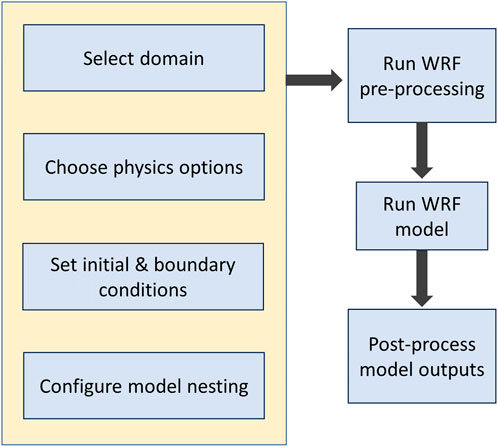
FIGURE 1. Flowchart showing the steps used to perform the WRF model simulations for this study.
The goals of this study are as follows:1) to quantify the predictability of an NWP model in capturing fire-weather; 2) to evaluate the sensitivity of the PBL scheme in capturing fire weather; and 3) to examine the effect of horizontal grid resolution on the prediction of meteorological parameters associated with a wildfire. We use the WRF model to simulate the weather conditions during the wildfire event. Our results will advance the understanding of optimal strategies for the operational forecast of fire-weather associated with large wildfires using mesoscale model simulations.
This study is organized into four main sections. Section 1 provides the background and motivation for this study. The data and methodology used to perform the sensitivity of PBL schemes and grid resolutions are presented in Section 2. Section 3 describes the results and discussion of our analysis. Conclusions are presented in Section 4.
We use the North American Regional Reanalysis (NARR) dataset (Mesinger et al., 2006) that is available at 12 km horizontal grid resolution and at every three hourly intervals to provide initial and boundary conditions to the WRF model (Skamarock et al., 2019). It is an extension of the National Centers for Environmental Prediction (NCEP) Global Reanalysis which is run over the North American Region. In this study, we run the model for 5 days, i.e., from 21 October 2007 to 26 October 2007. In addition, we use the hourly surface measurements (wind speed at 10 m, temperature at 2 m, and relative humidity at 2 m) from the U.S. Environmental Protection Agency (EPA) Air Quality System (AQS) data (https://www.epa.gov/aqs) for model validation. Meteorological data, such as the wind speed at 10 m, the temperature at 2 m, and relative humidity at 2 m, are extracted from individual AQS surface stations within the WRF innermost domain (d03 in Figure 2) for simulation evaluation. Finally, we use AmeriFlux (Kimberly Ann et al., 2018) data from the SCw station to compare surface heat and momentum flux observations against WRF predictions. Here, SCw represents the Southern California Climate Gradient - Pinyon/Juniper Woodland site.

FIGURE 2. The WRF Preprocessing configuration is shown in panel (A) with three different two-way nested domains (d01, d02, and d03). All the results in this study are shown for d03. Panel (B) shows the number and location of different stations used for the model validation for temperature, relative humidity, wind speed, and heat flux. The Witch Fire area is shown in panel (C) from San Diego County.
We use WRF model version 4.3.1 (Skamarock et al., 2019) with three two-way nested domains. The flowchart in Figure 1 shows the steps used to perform the model simulations for this study. The initial and boundary conditions for the model are provided from NARR data at every three hourly intervals. We choose two sets of PBL schemes, namely, the Yonsei University (abbreviated as YSU throughout this manuscript) (Hong et al., 2006) and the Mellor-Yamada-NakanishiNiino Level 2.5 scheme (abbreviated as MYNN throughout this manuscript) (Nakanishi and Niino, 2004) and combined with the two sets of grid resolutions. Therefore, we perform a total of four simulations as shown in Table 2 using various permutations of grid resolution and PBL schemes. During the simulation, we stored WRF outputs at every 1-h interval. We compare the results of all simulations with observations on an hourly basis.
All the simulations are initialized at the same time and run from 00 Z UTC (5 p.m. Pacific time) on October 21st to 00 Z UTC (5 p.m. Pacific time) on 26 October 2007, allowing 12 h for model spin-up and 4 days and 13 h for simulations. Two sets of horizontal grid resolutions are used for model set-up in our study: 9 km, 3 km, and 1 km and 36 km, 12 km, and 4 km for the outermost, middle, and innermost domains respectively. We used 33 vertical pressure levels with the top level at 13,706 m and the grid spacing is finer closer to the surface for all WRF simulations.
In the coarser grid experiments, the mesoscale domain (d01) has a horizontal extent of 3,240 km by 3,240 km, with 90 grid cells in both X and Y directions, while domain 2 (d02) has 151 grids in both X and Y directions with a domain size of 1812 km by 1812 km, and domain 3 (d03) has a horizontal extent of 1,084 km by 1,084 km, with 271 grid cells in both X and Y directions as shown in the summary Table 1. The time step for integration is 216 s for d01 in the coarser grid simulation. Since this ensures the model stability required for the simulation, it is recommended to set the time-step in the WRF model between 3*dx to 6*dx, where dx is in km for the outermost domain and the time-step is in seconds (Skamarock et al., 2005; Hutchinson, 2007). In the finer grid experiments, the mesoscale domain (d01) has a horizontal extent of 3,213 km by 3,213 km, with 357 grid cells in both X and Y directions, while domain 2 (d02) has 601 grids in both X and Y directions with a domain size of 1803 km by 1803 km, and domain 3 (d03) has a horizontal extent of 1,081 km by 1,081 km, with 1,081 grid cells in both X and Y directions. The time step for integration is 30 s for d01 in the finer grid simulations. The outputs for the innermost domain (d03) are stored at every hour and the parent time step ratio (outer/inner) is 3 for all simulations.

TABLE 1. The summary table shows the description of the domain grid specifications for coarser and finer domain model simulations used in this study.
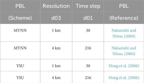
TABLE 2. The table shows the list of simulations performed for this study using two PBL scheme options (YSU and MYNN2.5) at two different horizontal grid resolutions (36 km, 12 km, 4 km and 9 km, 3 km, 1 km) in the WRF model. The ‘Resolution’ in the table represents the horizontal grid resolution and it is shown for the inner-most domain (d03) only.
For all simulations and domains, we used the following physical parameterizations: the rapid radiative transfer model (RRTM) (Mlawer et al., 1997) for the longwave radiation schemes and the Dudhia scheme for shortwave radiation (Dudhia, 1989); the revised MM5 scheme for surface physics (Jiménez et al., 2012); the unified NOAH land-surface model as the land surface (Mukul Tewari et al., 2004); the Purdue Lin scheme for cloud microphysics (Chen and Sun, 2002). Moreover, the soil moisture is a prognostic variable in the unified Noah land-surface model which is coupled with the WRF model. For the cumulus parameterization scheme, we choose the Grell 3D Ensemble scheme (Grell, 1993) for the two outermost domains in all experiments, while for the innermost domain, we do not use cumulus parameterization in any of the experiments.
While comparing WRF outputs at specific locations with the AQS surface station dataset, a few quality control criteria are established. As a gap-filling strategy, some stations embed repeated values of the last valid observation for specific variables. We filter out the repeated values of meteorological variables from the AQS data while calculating correlation statistics when it gets repeated for more than three continuous hours. Furthermore, we also filter out those stations that contain missing data values at one or more time instants.
The Python interpolation tool is used to extract the relevant meteorological variables from WRF outputs within the innermost domain of the model. We used an inverse distance weighted interpolation method to bring the model-simulated variable to the observation location. We used interpn from the scipy library to calculate the same. After quality control, For comparing hourly temperatures at 2 m height (T2), 90 AQS stations are used. For comparing hourly relative humidity at 2 m height (RH2), we use a total of 48 stations. Similarly, we use a total of 43 AQS stations for the purpose of comparing wind speed at 10 m height (WSPD10). Pearson’s correlation coefficient and the root mean square error (RMSE) statistics are used to evaluate these comparisons. One specific site near the Witch Fire location (site 1,006, Latitude 32.842242 N and Longitude −116.768225 W) is investigated in more detail, and the time series of T2, RH2, and Vapor Pressure Deficit (VPD) is compared against WRF outputs.
The Yonsei University scheme (YSU) (Hong et al., 2006) and the Mellor-Yamada-Nakanishi-Niino (MYNN) (Nakanishi and Niino, 2004) schemes are two of the most commonly used PBL schemes in the WRF model. Since the YSU PBL scheme expresses turbulence in terms of mean variables rather than additional prognostic variables, it is a first-order closure scheme. The YSU PBL scheme also incorporates an explicit treatment of the entrainment layer at the top of the PBL, which is an improvement to the medium range forecast (MRF) PBL scheme (Hong and Pan, 1996). The YSU scheme is also classified as a “non-local” scheme because, in addition to parameterizing the effect of turbulence caused by small eddies, it also considers transport caused by convective large eddies (Hong et al., 2006; Skamarock et al., 2008).
The MYNN scheme is based on a prognostic equation for turbulent kinetic energy (TKE) and is a 1.5-order local closure scheme (Nakanishi and Niino, 2004; Nakanishi and Niino, 2006). It is an improvement of the Mellor–Yamada–Janjic (MYJ) PBL scheme (Janić, 2001). The MYNN scheme uses the results from large eddy simulations (LES) to generate expressions of stability and mixing length as contrary to MYJ, which derives these expressions from observations (Cohen et al., 2015; Njuki et al., 2022). However, like other local closure schemes, the MYNN scheme does not account for deeper vertical mixing caused by large eddies (Cohen et al., 2015).
Surface heterogeneity and land-cover information are not adequately represented at the coarser resolution in the model. Therefore it is worth testing whether a finer grid resolution would capture the finer scale surface characteristics, which would enhance surface feedback processes and thereby affect the near-surface meteorology. The choice of grid resolution therefore should affect fire-weather simulations. Most of the operational weather prediction systems use 3 km–5 km horizontal grids for predicting local and regional weather conditions on an hourly to weekly basis. At the coarser resolution, the WRF model is unable to resolve some of the small-scale processes and effects of finer-scale features in weather prediction, such as clouds and turbulence, etc. In addition, models at such resolutions fail to capture the physical features. For example, near coastal regions, there is the presence of clouds and a coarser resolution model may not represent them well. Similarly, in the regions of complex topography, models do not resolve the orography well and thus fail to capture their effect on some of the underlying processes, resulting in a poor prediction.
The scattering diagram for temperature (T2) (panels a, b, c, d), relative humidity (RH2) (panels e, f, g, h), and wind speed (WSPD10) (panels i, j, k, l) for AQS surface stations in the innermost domain (d03) are shown in Figure 3. The R-squared value, R2, and RMSE for all variables are reported in Table 3.
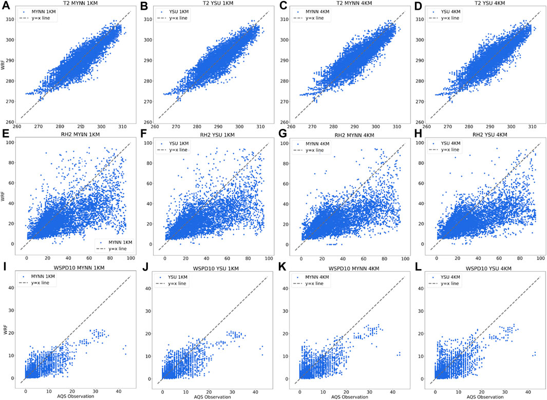
FIGURE 3. Scattering diagrams for T2, RH2, and WSPD10 for all the stations within the innermost domain (d03). The results are presented from 1 km to 4 km using YSU and MYNN PBL schemes and with the observational data (AQS) in order to show (A) T2 at 1 km for MYNN; (B) T2 at 1 km for YSU; (C) T2 at 4 km for MYNN; (D) T2 at 4 km for YSU; (E) RH2 at 1 km for MYNN; (F) RH2 at 1 km for YSU; (G) RH2 at 4 km for MYNN; (H) RH2 at 4 km for YSU; (I) WSPD10 at 1 km for MYNN; (J) WSPD10 at 1 km for YSU; (K) WSPD10 at 4 km for MYNN; and (L) WSPD10 at 4 km for YSU in the respective panels.
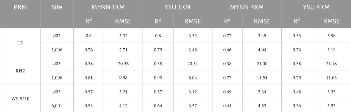
TABLE 3. The summary table showing RMSE and R2 values for T2, WSPD10, and RH2 from the different simulations at site 1,006, site 6,001, and for all stations combined within the d03 (inner-most domain) domain in California.
We find that there is an evidently strong correlation between the surface station observations and WRF outputs. The overall prediction of temperature at 2 m for all stations is sensitive to the horizontal grid resolution regardless of the choice of PBL schemes. Therefore, simulations with 1 km grid resolution are found to have a higher correlation for surface temperature compared to simulations with 4 km (Figure 3) resolution. For the coarser resolution simulations, the MYNN scheme yields a higher correlation in comparison to the YSU PBL scheme.
For relative humidity at 2 m height above the surface, correlations for all surface stations are quite lower than the surface temperature, and much more variability is observed in the datasets. However, no effective sensitivity to grid resolution or the choice of PBL scheme is noticed. The RMSE is slightly higher for the coarser resolution simulations for both PBL schemes.
For wind speed at 10 m height, the correlation between all surface station observations and WRF outputs for all four simulations is higher than relative humidity but lower than surface temperature. These correlations are also not as sensitive to PBL schemes but are strongly dependent on grid resolution with finer-scale simulations yield stronger correlations.
From Figure 3 and Table 3, we can generally conclude that while surface temperature and surface wind speed are captured relatively better than surface relative humidity, there is also a notable spread in the data while considering all weather stations in the inner domain of WRF. It is important to note that wind speed is in general underestimated. This is due to relatively coarse resolution even at 1 km grid cell size. Moreover, the choice of the PBL scheme does not have much impact on predicting meteorological parameters on the surface, although finer-scale simulations provide improved predictions. In the next section, we investigate the spatial variability captured by the WRF model by comparing the surface stations against WRF predictions.
The spatial variability of the correlation for the meteorological variables among the surface stations and WRF simulation of the Witch Fire event is depicted in Figure 4. We find that temperatures at 2 m are better captured over valleys than mountains. Coastal sites are associated with a lower correlation for temperature as shown with the lighter color in Figure 4. This could be because the model grid for coarser resolution simulations is situated partially on both land and ocean. Furthermore, the presence of clouds near the coastal regions could be another reason for poor model performance. It is important to note that MYNN performs relatively better than YSU at 4 km in capturing the spatial variability of temperature. Considerable spatial variability in the correlation coefficient is also found for relative humidity and surface wind speed. In the next section, we focus on one specific site (1,006) which is proximal to the Witch Fire location.
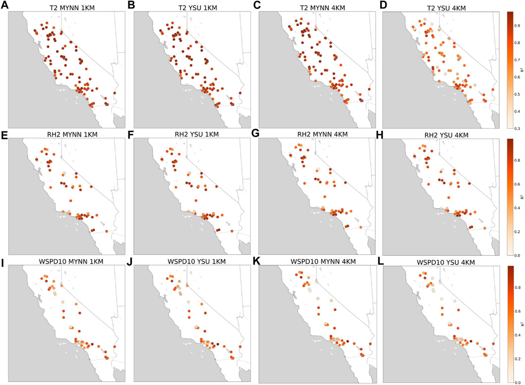
FIGURE 4. Location-wise plots for T2, RH2, and WSPD10 for all the stations within d03. The results are computed from 1 km to 4 km using YSU and MYNN PBL schemes and with the observational data (AQS) in order to show (A) T2 at 1 km for MYNN; (B) T2 at 1 km for YSU; (C) T2 at 4 km for MYNN; (D) T2 at 4 km for YSU; (E) RH2 at 1 km for MYNN; (F) RH2 at 1 km for YSU; (G) RH2 at 4 km for MYNN; (H) RH2 at 4 km for YSU; (I) WSPD10 at 1 km for MYNN; (J) WSPD10 at 1 km for YSU; (K) WSPD10 at 4 km for MYNN; and (L) WSPD10 at 4 km for YSU in the respective panels.
Table 3 also shows the correlations for station 1,006 [32.84 N, 116.77 W] along with the aggregated correlations for all sites as discussed before. It can be assumed that this station is influenced by the presence of the Witch Fire. It is interesting to note that while correlations for temperature are high for site 1,006, the correlations are greatly improved for relative humidity and wind speed compared to the aggregated correlations, at least for the higher-resolution simulations. Similar to the aggregated correlations, higher resolution simulations perform better than coarser resolution simulations for site 1,006 as well. Moreover, the YSU scheme performs better as evidenced by higher R2 and lower RMSE values compared to the MYNN scheme at site 1,006 except for wind speed at site 6,001 for the 4 km resolution simulations.
The mesoscale meteorological conditions and SAW gusts during the 2007 Witch Fire event intensified the fire spread and the fire intensity. To evaluate the ability of the WRF model to simulate the surface meteorological conditions of the fire, we compare modeled and observed time-series at the surface stations as shown in Figure 5. We observe that the performance of the WRF model is better in capturing the temporal variation of meteorological parameters at site 1,006 at 1 km resolution simulations for both MYNN and YSU PBL schemes as compared to at 4 km simulations (fire start time: 21 October 2007, at 19:35 UTC). The surface temperature and VPD are under-predicted by WRF, while the relative humidity is over-predicted at site 1,006 (Figure 5). No clear trend of under or over-prediction is observed for wind speed. The correlations for vapor pressure deficit are very high (>0.78) as well for all simulations. This observation is particularly interesting in the context of fire weather as VPD is a strong predictor for the hot and dry conditions that promote wildfire ignition and propagation.

FIGURE 5. Timeseries for T2, RH2, VPD, and WSPD10 for stations closer to the 2007 Witch Fire. The results are compared from 1 km to 4 km using YSU and MYNN PBL schemes with observations in order to show (A) T2 at site 1,006; (B) RH2 at site 1,006; (C) VPD at site 1,006; (D) Timeseries of Wind Speed at 10 m (Site 6001).
These results suggest that even without an explicit fire-weather parameterization, the WRF model is able to capture the meteorological conditions during a large wildfire event relatively well. In the next subsection, we investigate how well the surface sensible heat flux is captured.
The accurate representation of surface sensible heat flux is required for capturing fire-weather and fire-atmosphere interaction (Thapa et al., 2022). In this study, we use the parameterized sensible heat flux from the model, represented as SHFX (total flux and it is entirely sub-grid). Also, we compare the modeled sensible heat flux (SHFX) against the sensible heat flux reported by an AmeriFlux flux tower observatory nearest to the Witch Fire perimeter. The site has an elevation of 1,281 m with Latitude and Longitude of 33.6047 N and −116.4527 W respectively. This site is referred to as US-SCw: Southern California Climate Gradient–Pinyon/Juniper Woodland in the AmeriFlux tower data repository. This is the only available flux tower that had data recorded during the Witch Fire event. Although the site was not affected by the fire area/perimeter, it was close to the Witch Fire region as shown in Figure 2.
It is observed that even without an active coupled fire behavior-atmosphere interaction module switched on, the WRF model is able to capture the heat flux reasonably well as compared to the observations (Figure 6). However, the sensible heat flux is underestimated by WRF during the daytime. During the intense fire period (from the 18th hour of October 21 to the 0th hour of October 23), no obvious difference in the sensible heat flux can be observed. While comparing four modeled experiments, we find that the temporal variation of heat fluxes is similar. Therefore each set of the combined PBL scheme and grid resolution that we use in this study would be effective in simulating sensible heat fluxes.
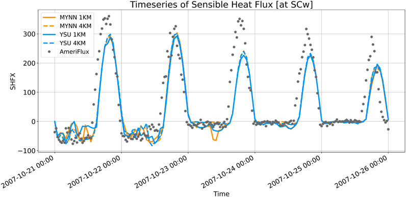
FIGURE 6. Timeseries of sensible heat flux [Wm−2] at SCw site (Southern California Climate Gradient - Pinyon/Juniper Woodland) from AmeriFlux tower and model simulation as shown in Table 2. This site has Latitude and Longitude values of 33.6047 N and 116.4527 W and the elevation is 1,281 m.
Since we test two different, widely used PBL schemes at two different grid resolutions of 1 km and 4 km, we investigate the PBL height variations for all four experiments over three different sites. In addition, we also focus on the PBL heights when the Witch Fire was highly intense, i.e., on 23rd October at 00:00 UTC (Figure 4). It is interesting to note that, MYNN estimates a higher mean PBL height at site 1,006 as compared to YSU at both 1 km, and 4 km grid resolutions (MYNN at 1 km = 372 m; MYNN at 4 km = 344 m; YSU at 1 km = 221 m; YSU at 4 km = 269 m) (top panel in Figure 7). The YSU PBL scheme estimates a higher mean PBL height at 4 km than at 1 km. However, for the MYNN, the mean PBL height is higher at 1 km as compared to at 4 km. Furthermore, the differences in the PBL heights are negligible for MYNN at both 4 km and 1 km during the intense fire period. We also find that during the period when the fire was intense, from the 18th hour of October 21 to the 0th hour of October 23, the variation in the PBL heights at SCw and at site 6,001 is much higher with the simulations at 4 km grid resolution than at 1 km (middle and bottom panel in Figure 7).
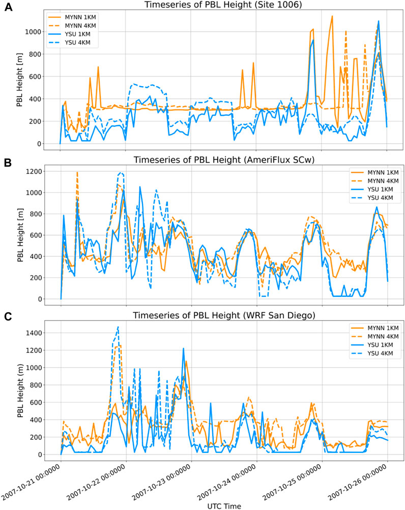
FIGURE 7. Timeseries plots for PBL heights for stations closer to the 2007 Witch Fire. The results are compared with 1 km and 4 km using YSU and MYNN PBL schemes to show (A) PBL at site 1,006; (B) PBL at a site called SCw (AmeriFlux); (C) Timeseries of PBL Height (Site 6001). These results are not compared with the observational data due to the data unavailability at those sites.
In this section, we compare the 10 m wind speed, and wind direction from all simulations at 12:00 UTC on 22 October 2007, i.e., during the period when the Witch Fire was highly intense. We find that the WRF model is able to simulate the direction of easterly winds, i.e., the surface wind flow for Santa Ana winds (Figures 8A–D). All simulations capture the winds from the mountains to the ocean, which is a characteristic of Santa Ana winds, regardless of the choice of PBL parameterization and horizontal grid resolution. This is captured well in all experiments regardless of the choice of PBL parameterization and horizontal grid resolution. In addition, the effects of the mountains on the wind are visible: the “canyon effect” (the wind is accelerated while passing through narrow canyons).
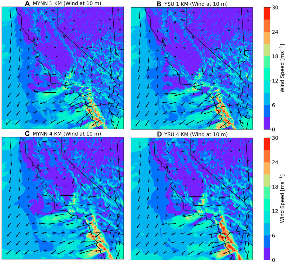
FIGURE 8. Wind speed (ms−1) and wind direction at 10 m for (A) MYNN 1 km; (B) YSU 1 km; (C) MYNN 4 km; (D) YSU 4 km as shown in Table 2. These plots are shown at 00 Z UTC (5 p.m. Pacific time) on 21 October 2007 when the fire is intense. The panels from (A) to (D) represent the entire innermost domain (d03) as shown in Figure 2.
The wind speed at 10 m has a higher magnitude over the ocean as well to the south of the San Diego coast and further in the ocean (Figures 8A–D). The magnitude is higher for YSU at 4 km (Figure 8D) as compared to the other cases (Figures 8A–C). Such strong wind over the ocean results from the influence of intensified 850 hPa wind conditions as described in section 3.3.2.
Spatial variation of wind speed is analyzed in section 3.1.2 and we find that the wind speed is predicted better at 1 km resolution due to a better representation of topography in the model. By comparing wind directions in Figures 8A–D, we observe that the vectors appear to be similar in direction and length for MYNN and PBL at 1 km and MYNN and YSU at 4 km. In addition, the model at 1 km generates higher wind speed over San Diego in Figures 8A,B when compared with Figures 8C,D. Thus, the choice of the horizontal grid has an impact on the wind direction and wind speed and the model performs reasonably well with a finer grid resolution.
In the wind field at 850 hPa (shown in Figure 9), there is a presence of intense and higher magnitude wind speed due to synoptic conditions. It is also evident that these synoptic wind conditions drive the surface wind which ultimately fanned the 2007 Witch Fire.
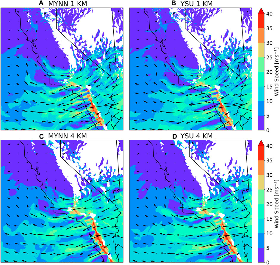
FIGURE 9. Wind speed (knot) and wind direction at 850 hPa for (A) MYNN 1 km; (B) YSU 1 km; (C) MYNN 4 km; (D) YSU 4 km as shown in Table 2. These plots are shown at 00 Z UTC (5 p.m. Pacific time) on 21 October 2007 when the fire is intense. The panels from (A) to (D) represent the entire innermost domain (d03) as shown in Figure 2.
We do not find any notable difference in the wind directions of four simulations as shown in Figures 9A–D. However, there are slight variations in the wind speed magnitude among the four sets of simulations. The 850 hPa winds across the mountain ridge result in mountain waves and downslope wind storms. The model captures the synoptic wind conditions that impact surface Santa Ana winds that fanned this Mega fire.
In this section, we analyze the vertical cross-section of wind speed and the vertical component of wind speed. Since from our analysis in the previous sections, it was determined that the wind speed is resolved well at the finer horizontal grid resolution, we present the vertical cross-section of wind speed from the MYNN PBL scheme only at 1 km as shown in Figure 10. In addition, this vertical cross-section is drawn at the latitude of 32.84 N which crosses the 2007 Witch Fire perimeter. The longitude varies from 120 W to 114.5 W to demonstrate the variation of wind speed across heights from land to ocean (Figure 10). The horizontal (Figure 10B) and vertical (Figure 10A) components of wind have a higher magnitude on the leeward side of the mountain range, which is a characteristic of the SAW events. The higher magnitude is because the standing mountain waves result in the leeward speed up, i.e., the downslope wind storm. In addition, a strong updraft is observed on the windward side of the mountain, as well as a strong downdraft on the leeward side. Thus, the model qualitatively demonstrates the wind conditions that are favorable for the intensification and a higher rate of spread of the 2007 Witch Fire. The area of higher wind speed coincides with the perimeter of the Witch Fire burned area (Lat: 32.87 N–32.88 N and Lon: 117.40 W–115.67 W). Since Figure 10 is shown at the instant when the fire was intense, we observe that the wind conditions are favorable for the intensification and a higher rate of spread for the Witch Fire.
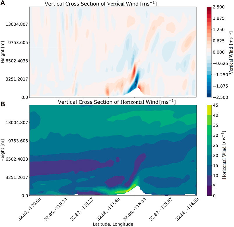
FIGURE 10. Vertical cross-section of (A) vertical wind (ms−1); (B) horizontal wind (ms−1) from MYNN at 1 km at 00 Z UTC (5 p.m. Pacific time) on 21 October 2007, when the fire is intense. In addition, this vertical cross section is drawn at the latitudinal value of 32.84 N which crosses the 2007 Witch Fire perimeter and longitudes from 120 W to 114.5 W.
This study investigated the WRF simulations of the 2007 Witch Fire event using two different and widely used PBL schemes, YSU and MYNN. In addition, we performed a sensitivity experiment with two different horizontal resolutions at 1 km and 4 km. The goal was to test the capability of the WRF model in simulating fire-weather and related conditions with different grid sizes and different PBL scheme combinations. We found that the model was able to capture fire-weather associated with the fire event with a reasonable accuracy close to the surface. On the other hand, the spatial and temporal variability of different meteorological parameters in the model were dependent on the grid resolutions and the choice of PBL schemes. In summary, the four simulations suggested that the model’s ability to predict near-surface meteorological conditions was improved at 1 km grid resolution compared to 4 km resolution. The results also indicated that wind is more difficult to capture than temperature and relative humidity even at a finer resolution of 1 km. One reason could be that 1 km resolution is not sufficient in highly complex terrain, the second reason is the representativeness of prediction vs. in situ point measurements, and the third could be the accuracy of PBL schemes. Furthermore, the performance of the MYNN scheme is found to be generally better than the YSU scheme.
The WRF model, capable of reasonably capturing meteorological parameters related to wildfires, can be further improved with the incorporation of the fire-atmosphere interaction module. Despite this enhancement, the grid resolution, even at 1 km, remains coarse, particularly for accurately resolving wind near complex topography. It is clear that coupling the WRF model with an active fire-atmosphere interaction component would significantly enhance its ability to resolve wildfire events. However, it is important to note that fire-atmosphere interaction models, while beneficial, are computationally prohibitive and necessitate resolutions close to 10 m for effective implementation in a coupled large eddy simulation mode. Therefore, the results of this study can be used to test the limits of the simple WRF model configuration to capture the effects of wildfire events. These results can provide the baseline over which the performance of more complex coupled WRF-Fire models can be tested.
The raw data supporting the conclusion of this article will be made available by the authors, without undue reservation.
MK: Conceptualization, Data curation, Formal Analysis, Funding acquisition, Investigation, Methodology, Project administration, Resources, Software, Validation, Visualization, Writing–original draft, Writing–review and editing. BK: Supervision, Writing–review and editing, Investigation. HN: Writing–review and editing, Data curation. WP: Investigation, Writing–review and editing. JR: Writing–review and editing, Investigation, Supervision. TB: Funding acquisition, Project administration, Supervision, Writing–review and editing.
The author(s) declare financial support was received for the research, authorship, and/or publication of this article. TB acknowledges funding support by the US National Science Foundation (NSF-AGS-PDM-2146520, NSF-OISE-2114740, NSF-CPS-2209695, NSF-ECO-CBET-2318718, and NSF-DMS-2335847), the University of California Office of the President (UCOP-LFR-20-653572), NASA (80NSSC22K1911), and the United States Department of Agriculture (NIFA 2021-67022-35908, and USDA-20-CR-11242306-072). BK’s contribution was supported by the NCAR, which is a major facility sponsored by the National Science Foundation under Cooperative Agreement No. 1852977. The authors acknowledge the National Oceanic and Atmospheric Administration (NOAA) for providing National Centers for Environmental Prediction (NCEP) reanalysis data. MK acknowledges the funding support from the Dean’s Dissertation Fellowship award from the Henry Samueli School of Engineering at the University of California Irvine, and the Research Applications Laboratory visitor grant from the National Center for Atmospheric Research (NCAR). TB also acknowledges funding support from the University of California Office of the President (UCOP) grant LFR-20-653572 (UC Lab-Fees); the National Science Foundation (NSF) grants NSF-AGS-PDM-2146520 (CAREER), NSF-OISE-2114740 (AccelNet) and NSF-CPS-2209695; the United States Department of Agriculture (USDA) grant 2021-67022-35908 (NIFA); and a cost reimbursable agreement with the USDA Forest Service 20-CR-11242306-072. Additional support was provided by the new faculty start-up grant provided by the Department of Civil and Environmental Engineering, the Henry Samueli School of Engineering, University of California, Irvine.
The authors declare that the research was conducted in the absence of any commercial or financial relationships that could be construed as a potential conflict of interest.
All claims expressed in this article are solely those of the authors and do not necessarily represent those of their affiliated organizations, or those of the publisher, the editors and the reviewers. Any product that may be evaluated in this article, or claim that may be made by its manufacturer, is not guaranteed or endorsed by the publisher.
Andrews, P., Finney, M., and Fischetti, M. (2007). Predicting wildfires. Sci. Am. 297 (2), 46–55. doi:10.1038/scientificamerican0807-46
Andrews, P. L. (2007). “Behaveplus fire modeling system: past, present, and future,” in Proceedings of 7th symposium on fire and forest meteorology (Boston MA: American Meteorological Society), 23–25.
Benjamin, S. G., Weygandt, S. S., Brown, J. M., Hu, M., Alexander, C. R., Smirnova, T. G., et al. (2016). A north american hourly assimilation and model forecast cycle: the rapid refresh. Mon. Weather Rev. 144 (4), 1669–1694. doi:10.1175/mwr-d-15-0242.1
Bowman, D. M., Balch, J., Artaxo, P., Bond, W. J., Cochrane, M. A., D’antonio, C. M., et al. (2011). The human dimension of fire regimes on earth. J. Biogeogr. 38 (12), 2223–2236. doi:10.1111/j.1365-2699.2011.02595.x
Bowman, D. M., Kolden, C. A., Abatzoglou, J. T., Johnston, F. H., van der Werf, G. R., and Flannigan, M. (2020). Vegetation fires in the anthropocene. Nat. Rev. Earth Environ. 1 (10), 500–515. doi:10.1038/s43017-020-0085-3
Brewer, M. J., and Clements, C. B. (2019). The 2018 camp fire: meteorological analysis using in situ observations and numerical simulations. Atmosphere 11 (1), 47. doi:10.3390/atmos11010047
Bryan, G. H., and Fritsch, J. M. (2002). A benchmark simulation for moist nonhydrostatic numerical models. Mon. Weather Rev. 130 (12), 2917–2928. doi:10.1175/1520-0493(2002)130<2917:absfmn>2.0.co;2
Burke, M., Driscoll, A., Heft-Neal, S., Xue, J., Burney, J., and Wara, M. (2021). The changing risk and burden of wildfire in the United States. Proc. Natl. Acad. Sci. 118 (2), e2011048118. doi:10.1073/pnas.2011048118
Cannon, S. H., and DeGraff, J. (2009). “The increasing wildfire and post-fire debris-flow threat in western USA, and implications for consequences of climate change,” in Landslides–disaster risk reduction (Springer), 177–190.
Cao, Y., and Fovell, R. G. (2016). Downslope windstorms of san diego county. part i: a case study. Mon. Weather Rev. 144 (2), 529–552. doi:10.1175/mwr-d-15-0147.1
Cao, Y., and Fovell, R. G. (2018). Downslope windstorms of san diego county. part ii: physics ensemble analyses and gust forecasting. Weather Forecast. 33 (2), 539–559. doi:10.1175/waf-d-17-0177.1
Chen, S.-H., and Sun, W.-Y. (2002). A one-dimensional time dependent cloud model. J. Meteorological Soc. Jpn. Ser. II 80 (1), 99–118. doi:10.2151/jmsj.80.99
Clarke, H., Evans, J. P., and Pitman, A. J. (2013). Fire weather simulation skill by the weather research and forecasting (wrf) model over south-east Australia from 1985 to 2009. Int. J. Wildland Fire 22 (6), 739–756. doi:10.1071/wf12048
Coen, J. (2018). Some requirements for simulating wildland fire behavior using insight from coupled weather—wildland fire models. Fire 1 (1), 6. doi:10.3390/fire1010006
Coen, J. L., Cameron, M., Michalakes, J., Patton, E. G., Riggan, P. J., and Yedinak, K. M. (2013). Wrf-fire: coupled weather–wildland fire modeling with the weather research and forecasting model. J. Appl. Meteorology Climatol. 52 (1), 16–38. doi:10.1175/jamc-d-12-023.1
Cohen, A. E., Cavallo, S. M., Coniglio, M. C., and Brooks, H. E. (2015). A review of planetary boundary layer parameterization schemes and their sensitivity in simulating southeastern us cold season severe weather environments. Weather Forecast. 30 (3), 591–612. doi:10.1175/waf-d-14-00105.1
Collins, S. N., James, R. S., Ray, P., Chen, K., Lassman, A., and Brownlee, J. (2013). Grids in numerical weather and climate models. Climate change and regional/local responses, 256.
Cruz, M. G., and Alexander, M. E. (2013). Uncertainty associated with model predictions of surface and crown fire rates of spread. Environ. Model. Softw. 47, 16–28. doi:10.1016/j.envsoft.2013.04.004
Di Giuseppe, F., Pappenberger, F., Wetterhall, F., Krzeminski, B., Camia, A., Libertá, G., et al. (2016). The potential predictability of fire danger provided by numerical weather prediction. J. Appl. Meteorology Climatol. 55 (11), 2469–2491. doi:10.1175/jamc-d-15-0297.1
Dudhia, J. (1989). Numerical study of convection observed during the winter monsoon experiment using a mesoscale two-dimensional model. J. Atmos. Sci. 46 (20), 3077–3107. doi:10.1175/1520-0469(1989)046<3077:nsocod>2.0.co;2
Duine, G.-J., Jones, C., Carvalho, L. M., and Fovell, R. G. (2019). Simulating sundowner winds in coastal santa barbara: model validation and sensitivity. Atmosphere 10 (3), 155. doi:10.3390/atmos10030155
Finney, M. A. (1998). FARSITE, Fire Area Simulator–model development and evaluation (US Forest Service: US Department of Agriculture, Forest Service, Rocky Mountain Research Station). Number 4.
Fovell, R. G., Brewer, M. J., and Garmong, R. J. (2022). The december 2021 marshall fire: predictability and gust forecasts from operational models. Atmosphere 13 (5), 765. doi:10.3390/atmos13050765
Fovell, R. G., and Cao, Y. (2017). The santa ana winds of southern California: winds, gusts, and the 2007 witch fire. Wind Struct. 24 (6), 529–564.
Giunta, G., Salerno, R., Ceppi, A., Ercolani, G., and Mancini, M. (2019). Effects of model horizontal grid resolution on short-and medium-term daily temperature forecasts for energy consumption application in european cities. Adv. Meteorology 2019, 1–12. doi:10.1155/2019/1561697
Grell, G. A. (1993). Prognostic evaluation of assumptions used by cumulus parameterizations. Mon. weather Rev. 121 (3), 764–787. doi:10.1175/1520-0493(1993)121<0764:peoaub>2.0.co;2
Hong, S.-Y., Noh, Y., and Dudhia, J. (2006). A new vertical diffusion package with an explicit treatment of entrainment processes. Mon. weather Rev. 134 (9), 2318–2341. doi:10.1175/mwr3199.1
Hong, S.-Y., and Pan, H.-L. (1996). Nonlocal boundary layer vertical diffusion in a medium-range forecast model. Mon. weather Rev. 124 (10), 2322–2339. doi:10.1175/1520-0493(1996)124<2322:nblvdi>2.0.co;2
Hutchinson, T. A. (2007). “An adaptive time-step for increased model efficiency,” in Extended abstracts (Eighth WRF Users’ Workshop), 4.
Janić, Z. I. (2001). Nonsingular implementation of the mellor-yamada level 2.5 scheme in the ncep meso model. NCEP Off. Note.
Jiménez, P. A., Dudhia, J., González-Rouco, J. F., Navarro, J., Montávez, J. P., and García-Bustamante, E. (2012). A revised scheme for the wrf surface layer formulation. Mon. weather Rev. 140 (3), 898–918. doi:10.1175/mwr-d-11-00056.1
Jiménez, P. A., Muñoz-Esparza, D., and Kosović, B. (2018). A high resolution coupled fire–atmosphere forecasting system to minimize the impacts of wildland fires: Applications to the chimney tops ii wildland event. Atmosphere 9 (5), 197. doi:10.3390/atmos9050197
Jin, Y., Goulden, M. L., Faivre, N., Veraverbeke, S., Sun, F., Hall, A., et al. (2015). Identification of two distinct fire regimes in southern California: implications for economic impact and future change. Environ. Res. Lett. 10 (9), 094005. doi:10.1088/1748-9326/10/9/094005
Juliano, T. W., Lareau, N., Frediani, M. E., Shamsaei, K., Eghdami, M., Kosiba, K., et al. (2023). Toward a better understanding of wildfire behavior in the wildland-urban interface: a case study of the 2021 marshall fire. Geophys. Res. Lett. 50 (10), e2022GL101557. doi:10.1029/2022gl101557
Keeley, J. E., and Syphard, A. D. (2019). Twenty-first century California, USA, wildfires: fuel-dominated vs. wind-dominated fires. Fire Ecol. 15 (1), 24–15. doi:10.1186/s42408-019-0041-0
Kumar, M. (2022). Mapping and modeling of fires in the wildland-urban interface. Irvine: University of California.
Kumar, M., Li, S., Nguyen, P., and Banerjee, T. (2022). Examining the existing definitions of wildland-urban interface for California. Ecosphere 13 (12), e4306. doi:10.1002/ecs2.4306
Kimberly Ann, N., Biederman, J. A., Desai, A. R. , Litvak, M. E., JP Moore, D., Scott, R. L., et al. (2018). The AmeriFlux network: A coalition of the willing. Agricultural and Forest Meteorology 249, 444–456.
Lagouvardos, K., Kotroni, V., Giannaros, T. M., and Dafis, S. (2019). Meteorological conditions conducive to the rapid spread of the deadly wildfire in eastern attica, Greece. Bull. Am. Meteorological Soc. 100 (11), 2137–2145. doi:10.1175/bams-d-18-0231.1
Lindley, T., Speheger, D. A., Day, M. A., Murdoch, G. P., Smith, B. R., Nauslar, N. J., et al. (2019). Megafires on the southern great plains. J. Operational Meteorology 7 (12), 164–179. doi:10.15191/nwajom.2019.0712
Linn, R., Reisner, J., Colman, J. J., and Winterkamp, J. (2002). Studying wildfire behavior using firetec. Int. J. wildland fire 11 (4), 233–246. doi:10.1071/wf02007
Lu, W., Zhong, S., Charney, J., Bian, X., and Liu, S. (2012). Wrf simulation over complex terrain during a southern California wildfire event. J. Geophys. Res. Atmos. 117 (D5). doi:10.1029/2011jd017004
Mallia, D. V., Kochanski, A. K., Kelly, K. E., Whitaker, R., Xing, W., Mitchell, L. E., et al. (2020). Evaluating wildfire smoke transport within a coupled fire-atmosphere model using a high-density observation network for an episodic smoke event along Utah’s wasatch front. J. Geophys. Res. Atmos. 125 (20), e2020JD032712. doi:10.1029/2020jd032712
Masoudvaziri, N., Bardales, F. S., Keskin, O. K., Sarreshtehdari, A., Sun, K., and Elhami-Khorasani, N. (2021). Streamlined wildland-urban interface fire tracing (swuift): modeling wildfire spread in communities. Environ. Model. Softw. 143, 105097. doi:10.1016/j.envsoft.2021.105097
Mell, W., Maranghides, A., McDermott, R., and Manzello, S. L. (2009). Numerical simulation and experiments of burning douglas fir trees. Combust. Flame 156 (10), 2023–2041. doi:10.1016/j.combustflame.2009.06.015
Mesinger, F., DiMego, G., Kalnay, E., Mitchell, K., Shafran, P. C., Ebisuzaki, W., et al. (2006). North american regional reanalysis. Bull. Am. Meteorological Soc. 87 (3), 343–360. doi:10.1175/bams-87-3-343
Mlawer, E. J., Taubman, S. J., Brown, P. D., Iacono, M. J., and Clough, S. A. (1997). Radiative transfer for inhomogeneous atmospheres: rrtm, a validated correlated-k model for the longwave. J. Geophys. Res. Atmos. 102 (D14), 16663–16682. doi:10.1029/97jd00237
Mölders, N. (2008). Suitability of the weather research and forecasting (wrf) model to predict the june 2005 fire weather for interior Alaska. Weather Forecast. 23 (5), 953–973. doi:10.1175/2008waf2007062.1
Mukul Tewari, N., Tewari, M., Chen, F., Wang, W., Dudhia, J., LeMone, M., et al. (2004). “Implementation and verification of the unified noah land surface model in the wrf model (formerly paper number 17.5),” in Proceedings of the 20th Conference on Weather Analysis and Forecasting/16th Conference on Numerical Weather Prediction, Seattle, WA, USA.
Nakanishi, M., and Niino, H. (2004). An improved mellor–yamada level-3 model with condensation physics: its design and verification. Boundary-layer Meteorol. 112 (1), 1–31. doi:10.1023/b:boun.0000020164.04146.98
Nakanishi, M., and Niino, H. (2006). An improved mellor–yamada level-3 model: its numerical stability and application to a regional prediction of advection fog. Boundary-Layer Meteorol. 119 (2), 397–407. doi:10.1007/s10546-005-9030-8
Neary, D. G. (2022). “Recent megafires provide a tipping point for desertification of conifer ecosystems,” in Conifers-recent advances (IntechOpen).
Njuki, S. M., Mannaerts, C. M., and Su, Z. (2022). Influence of planetary boundary layer (pbl) parameterizations in the weather research and forecasting (wrf) model on the retrieval of surface meteorological variables over the kenyan highlands. Atmosphere 13 (2), 169. doi:10.3390/atmos13020169
Raphael, M. (2003). The santa ana winds of California. Earth Interact. 7 (8), 1–13. doi:10.1175/1087-3562(2003)007<0001:tsawoc>2.0.co;2
Skamarock, W. C., Klemp, J. B., Dudhia, J., Gill, D. O., Barker, D. M., Wang, W., et al. (2005). A description of the advanced research wrf version 2. Technical report. National Center For Atmospheric Research Boulder Co Mesoscale and Microscale.
Skamarock, W. C., Klemp, J. B., Dudhia, J., Gill, D. O., Barker, D. M., Wang, W., et al. (2008). A description of the advanced research wrf version 3. ncar technical note-475+ str. Boulder, CO, USA: National Center for Atmospheric Research.
Skamarock, W. C., Klemp, J. B., Dudhia, J., Gill, D. O., Liu, Z., Berner, J., et al. (2019). A description of the advanced research wrf model version 4, 145. Boulder, CO, USA: National Center for Atmospheric Research, 145.
Stephens, S. L., Collins, B. M., Biber, E., and Fulé, P. Z. (2016). Us federal fire and forest policy: emphasizing resilience in dry forests. Ecosphere 7 (11), e01584. doi:10.1002/ecs2.1584
Stephens, S. L., and Ruth, L. W. (2005). Federal forest-fire policy in the United States. Ecol. Appl. 15 (2), 532–542. doi:10.1890/04-0545
Sullivan, A. L. (2009). Wildland surface fire spread modelling, 1990–2007. 1: physical and quasi-physical models. Int. J. Wildland Fire 18 (4), 349–368. doi:10.1071/wf06143
Thapa, L. H., Ye, X., Hair, J. W., Fenn, M. A., Shingler, T., Kondragunta, S., et al. (2022). Heat flux assumptions contribute to overestimation of wildfire smoke injection into the free troposphere. Commun. Earth Environ. 3 (1), 236–311. doi:10.1038/s43247-022-00563-x
Varga, K., Jones, C., Trugman, A., Carvalho, L. M., McLoughlin, N., Seto, D., et al. (2022). Megafires in a warming world: what wildfire risk factors led to California’s largest recorded wildfire. Fire 5 (1), 16. doi:10.3390/fire5010016
Wang, B., Spessa, A. C., Feng, P., Hou, X., Yue, C., Luo, J.-J., et al. (2022). Extreme fire weather is the major driver of severe bushfires in southeast Australia. Sci. Bull. 67 (6), 655–664. doi:10.1016/j.scib.2021.10.001
Wedi, N. P. (2014). Increasing horizontal resolution in numerical weather prediction and climate simulations: illusion or panacea? Philosophical Trans. R. Soc. A Math. Phys. Eng. Sci. 372 (2018), 20130289. doi:10.1098/rsta.2013.0289
Keywords: fire-weather, grid resolution, nesting, PBL scheme, wildfires, WRF (weather research and forecasting)
Citation: Kumar M, Kosović B, Nayak HP, Porter WC, Randerson JT and Banerjee T (2024) Evaluating the performance of WRF in simulating winds and surface meteorology during a Southern California wildfire event. Front. Earth Sci. 11:1305124. doi: 10.3389/feart.2023.1305124
Received: 30 September 2023; Accepted: 14 December 2023;
Published: 19 January 2024.
Edited by:
Chenghao Wang, University of Oklahoma, United StatesReviewed by:
Rosmeri Porfirio Da Rocha, University of São Paulo, BrazilCopyright © 2024 Kumar, Kosović, Nayak, Porter, Randerson and Banerjee. This is an open-access article distributed under the terms of the Creative Commons Attribution License (CC BY). The use, distribution or reproduction in other forums is permitted, provided the original author(s) and the copyright owner(s) are credited and that the original publication in this journal is cited, in accordance with accepted academic practice. No use, distribution or reproduction is permitted which does not comply with these terms.
*Correspondence: Mukesh Kumar, bXVrZXNoa0B1Y2kuZWR1
†Present address: Mukesh Kumar, Earth and Environmental Sciences Division, Los Alamos National Laboratory, Los Alamos, NM, United States
Disclaimer: All claims expressed in this article are solely those of the authors and do not necessarily represent those of their affiliated organizations, or those of the publisher, the editors and the reviewers. Any product that may be evaluated in this article or claim that may be made by its manufacturer is not guaranteed or endorsed by the publisher.
Research integrity at Frontiers
Learn more about the work of our research integrity team to safeguard the quality of each article we publish.