Combining Karhunen–Loève expansion and stochastic modeling for probabilistic delineation of well capture zones in heterogeneous aquifers

The delineation of well capture zones (WCZs), particularly for water supply wells, is of utmost importance to ensure water quality. This task requires a comprehensive understanding of the aquifer’s hydrogeological parameters for precise delineation. However, the inherent uncertainty associated with these parameters poses a significant challenge. Traditional deterministic methods bear inherent risks, emphasizing the demand for more resilient and probabilistic techniques. This study introduces a novel approach that combines the Karhunen–Loève expansion (KLE) technique with stochastic modeling to probabilistically delineate well capture zones in heterogeneous aquifers. Through numerical examples involving moderate and strong heterogeneity, the effectiveness of KLE dimension reduction and the reliability of stochastic simulations are explored. The results show that increasing the number of KL-terms significantly improves the statistical attributes of the samples. When employing more KL-terms, the statistical properties of the hydraulic conductivity field outperform those of cases with fewer KL-terms. Notably, particularly in scenarios of strong heterogeneity, achieving a convergent probabilistic WCZs map requires a greater number of KL-terms and stochastic simulations compared to cases with moderate heterogeneity.

1 Introduction

Well capture zones have undergone significant evolution as our understanding of groundwater flow and contaminant transport processes has grown. Early approaches, such as the fixed-radius method and analytical methods (EPA, 1994; Shan, 1999; Christ and Goltz, 2002; Fienen et al., 2005), were relatively simplistic; however, they failed to account for the uncertainties inherent in the groundwater system and potential contaminant sources. Consequently, these approaches exhibited limitations in providing reliable and robust protection measures for well capture zones.

To address the demand for enhanced accuracy and reliability in well capture zone protection strategies, significant progress has been achieved in the field of hydrogeology and contaminant transport (Jiang et al., 2019; Zhu et al., 2019). Among the approaches, the Particle Tracking (PT) method (Rock and Kupfersberger, 2002; Barry et al., 2009; Nalarajan et al., 2019) has gained prominence among hydrogeologists. This method entails utilizing groundwater modeling codes to establish flow systems and subsequently tracking particles along flow paths to delineate well capture zones or travel time areas. Nevertheless, it’s important to note that conventional PT methods often neglect the consideration of uncertainties.

To address this challenge, one approach is to embed Particle Tracking (PT) within a Monte Carlo framework (PTMC) (Hunt et al., 2001; Frind and Molson, 2018; Moeck et al., 2020). By incorporating Monte Carlo methods, PTMC can evaluate the well capture zones (WCZs) while accounting for uncertainties. This is accomplished by simulating possible variations in the flow system and different flow paths. Each realization represents one possible state of the aquifer system, and aggregating the outcomes of all realizations provides a more comprehensive and reliable assessment of WCZs.

While embedding Particle Tracking within a Monte Carlo framework (PTMC) offers a degree of uncertainty consideration, the representation of uncertainty associated with the site’s hydraulic conductivity can still be relatively simplistic. Often, this relies on homogeneous or zonal approaches (Qiao et al., 2015; Mohebbi Tafreshi et al., 2019). The homogeneous approach assumes a uniform hydraulic conductivity across the entire aquifer, which could be suitable for specific cases but might oversimplify the complexity of most sites. The zonal approach seeks to delineate different hydraulic conductivity values in distinct regions or layers to better reflect spatial heterogeneity realistically. However, the zonal approach may not fully capture the true spatial variability of the hydraulic conductivity.

When dealing with uncertainty in hydraulic conductivity, a more sophisticated and accurate approach involves the use of geostatistical modeling methods (Turcke and Kueper, 1996; Patriarche et al., 2005; Jiang et al., 2021). This technique can generate numerous equiprobable realizations of the hydraulic conductivity by considering the spatial variability of geological data. These realizations can subsequently be integrated into groundwater models to analyze well capture zones. However, geostatistical modeling methods [such as SGSIM, (Pebesma and Wesseling, 1998)] require substantial computational resources when performing extensive site characterization that relies on statistical information.

To improve the computational efficiency, various methods for generating hydraulic conductivity fields have been proposed, including the Fourier transform method (Robin et al., 1993), wavelet transform method (Haßler et al., 2011), Principal component analysis method. Among these, the Fourier transform lacks flexibility dealing with isotropy, and the choice of the wavelet function has significant impact on the results of the wavelet transform. In recent years, the Principal Component Analysis (PCA) method is commonly employed for reducing the dimensionality of hydraulic conductivity fields. By applying PCA, the hydraulic conductivity field can be represented with fewer principal components while preserving the essential information and spatial variability inherent in the original data. The Karhunen-Loève Expansion (KLE) method (Ding et al., 2008; Xue et al., 2018; Zhang et al., 2018), a widely used variant of PCA, is particularly well-suited for handling geologic attribute data characterized by strong spatial correlation. Through eigenvalue decomposition of the random field, KLE generates a set of orthogonal functions that characterize the primary variation modes within the random field, similar to standard PCA. By selecting the leading principal components, effective dimensionality reduction can be achieved.

Previous studies have predominantly relied on the zonal method to describe heterogeneity, which often falls short of accurately capturing the true complexity of natural systems. This study aims to advance our understanding of hydraulic conductivity heterogeneity by adopting the spatial field perspective, albeit at the cost of increased dimensionality in the problem to be solved. To address this challenge, we integrate the dimensionality reduction techniques of Principal Component Analysis (PCA), particularly the Karhunen-Loève Expansion (KLE), with the stochastic simulation method to conduct a delineation study of well capture zones (WCZs) within heterogeneous aquifers. This study spans various aspects, including the methodological framework, the effectiveness of KLE-based dimension reduction, and the reliability of stochastic simulations.

The remainder of this paper is organized as follows. Section 2 provides a comprehensive description of groundwater flow model and the MODPATH program. It also outlines the methodologies employed, which include Karhunen-Loève expansion method and the Monte Carlo simulation method. Section 3 presents an illustrative example to contextualize this study. In Section 4, the results obtained from numerical experiments are discussed. Concluding remarks are given in Section 5.

2 Methods

This section provides an overview of the physical process (Section 2.1) in this study as well as the methodologies employed, including Karhunen-Loève (KL) expansion technique for generating the hydraulic conductivity field (Section 2.2), and the Monte Carlo simulation method (Section 2.3).

2.1 Problem formulation

In this study, a groundwater flow model was constructed using the MODFLOW module in Flopy (Bakker et al., 2016). Utilizing this groundwater flow model, we employed the particle tracking technique from the MODPATH module to determine the sources of groundwater recharge for supply wells within a specified period of time.

The governing equation for steady-state groundwater flow is expressed as follows:

$\frac{\partial }{{\partial \mathit{x}}_{\mathit{i}}}\left({\mathit{K}}_{\mathit{i}\mathit{j}}\frac{\partial \mathit{h}}{{\partial \mathit{x}}_{\mathit{j}}}\right)+\mathbf{\epsilon }=\mathbf{0}i,j=\mathrm{1,2},(1)$

and the flow velocity v [LT⁻¹] can be obtained using Darcy’s law:

${\mathit{v}}_{\mathit{i}}=-\frac{{\mathit{K}}_{\mathit{i}\mathit{j}}}{\mathrm{\theta }}\frac{\partial \mathit{h}}{{\partial \mathit{x}}_{\mathit{j}}}i,j=\mathrm{1,2},(2)$

Where h [L] is the hydraulic head; $K_{ij}$ [LT⁻¹] represents the hydraulic conductivity; x_i and x_j represent the Cartesian coordinates; $\mathrm{\epsilon }$ [T^-1] is volumetric flux per unit volume representing sources and/or sinks of water; θ is effective porosity (dimensionless). The governing equation for flow is solved using the numerical simulator MODFLOW (Harbaugh et al., 2000).

MODPATH (Pollock, 2016) is a specialized program used for particle tracking simulations in groundwater studies. The flowline tracing capability of MODPATH, particularly its backward tracking technique, can be employed to identify the recharge area of pumping wells. For two-dimensional steady flow, the mass balance equation of MODPATH can be expressed as:

$\frac{\partial }{{\partial x}_1}\left(\theta v_1\right)+\frac{\partial }{{\partial x}_2}\left(\theta v_2\right)=W,(3)$

where $v_1$ and $v_2$ are the principal components of the average linear groundwater velocity vector, W is the volume rate of water created or consumed by internal sources and sinks per unit volume of aquifer.

2.2 Generation of hydraulic conductivity field

Given the intricate and uncertain nature of real geological media, the utilization of random fields, or spatially correlated random variables, becomes essential to depict the spatial distribution attributes of specific geological media. Hydraulic conductivity, a significant parameter influencing groundwater flow and contaminant transport, demands the generation of a well-founded hydraulic conductivity field for robust uncertainty analysis. Extensive research has corroborated that hydraulic conductivity fields adhere to a log-normal distribution (Turcke and Kueper, 1996; Lu et al., 2017) in spatial context.

In the field of hydrogeology, the Karhunen-Loève (KL) expansion method (Zhang and Lu, 2004) serves as an extensively used technique for the generation of random fields. This approach enables the generation of multiple realizations of random fields that conform to the statistical attributes and spatial structure of the observed data. In this study, the Karhunen-Loève (KL) expansion method was adopted for generating the hydraulic conductivity field.

Let $\mathrm{Y}\left(x,\omega \right)=\mathit{ln}K\left(x,\omega \right)$ be a random event, where $x\in D$ and $\omega \in \mathrm{\Omega }$ (a probability space). $⟨\mathrm{Y}\left(x,\omega \right)⟩$ denotes the mean component of $\mathrm{Y}\left(x,\omega \right)$ over all possible realizations of the process. A covariance function $C\left(x,y\right)$, which is bounded, symmetric and positive definite, is required to be specified to construct the KLE and it can be decomposed into:

$C\left(x,y\right)={\displaystyle \sum _{i=1}^{\infty }}{\tau }_i{f}_i\left(x\right)f_i\left(y\right),(4)$

Where ${\tau }_i$ and $f_i\left(x\right)$ are eigenvalues and eigenfunctions of the correlation function, respectively and can be solved according to the second kind of the homogeneous Fredholm integral equation.

The random process $\mathrm{Y}\left(x,\omega \right)$ can be expanded as:

$\mathrm{Y}\left(x,\omega \right)=〈\mathrm{Y}\left(x,\omega \right)〉+{\displaystyle \sum _{i=1}^{\infty }}{\xi }_i\sqrt{{\tau }_i}{f}_i\left(x,\omega \right),(5)$

Where ${\xi }_i$ are independent standard Gaussian random variables. The finite-dimensional approximation of the log-conductivity and log-distribution coefficient field can be given by truncating N_KL terms of Eq. 5.

$\mathrm{Y}\left(x,\omega \right)\approx 〈\mathrm{Y}\left(x,\omega \right)〉+{\displaystyle \sum _{i=1}^{N_{KL}}}{\xi }_i\sqrt{{\tau }_i}{f}_i\left(x,\omega \right),(6)$

2.3 Monte Carlo simulation method

Any model-based risk assessment inherently involves uncertainties. In the WCZs problem, the incorporation of spatial probability maps can be a viable approach for delineating the protection areas, which represent the regions that may pose risks to water supply wells.

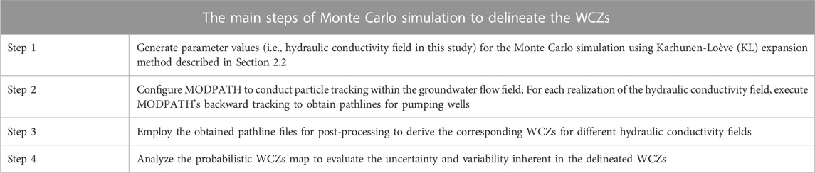
The Monte Carlo simulation method is employed in this study to analyze model uncertainties. In scenarios involving prior information, the Monte Carlo method is utilized to statistically estimate the probability of a specific random event. This process transforms uncertainty within the random model parameters of hydraulic conductivities into uncertainty within model outcomes, thereby facilitating uncertainty analysis of WCZs through statistical techniques. The main steps of our approach are outlined as follows:

3 Illustrative examples

In this study, we investigate a hypothetical aquifer that is saturated and confined. The aquifer has a fixed thickness of 10 m and spans a distance of 800 m from east to west and 400 m from north to south. To model this aquifer, a square grid with dimensions of 10 × 10 m² was employed, resulting in a total of 40 rows and 80 columns.

The boundary conditions were established for both the upgradient (West) and downgradient (East) regions. At the upgradient boundary (x = 0 m), a hydraulic head of 15 m was specified, whereas at the downgradient boundary (x = 800 m), a hydraulic head of 10 m was assigned. Consequently, an average hydraulic gradient of 0.625% was derived between these two boundary points. The North boundary (y = 500 m) and the South boundary (y = 0 m) were considered impermeable, as depicted in Figure 1. Additionally, a single pumping well was positioned at the coordinates of row 21 and column 62, with a flow rate of 100 m³/d. For the sake of simplicity, a uniform porosity value of 0.30 was assumed for the aquifer, and the flow system was in a steady state.

FIGURE 1

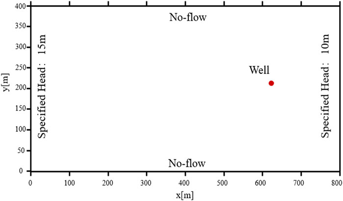
FIGURE 1. An illustration of the study area.

Considering the main objective of this study is to understand the impact of spatial variability on the delineation of WCZs and evaluate the associated probability risks, WCZs were calculated using both deterministic and stochastic modeling approaches.

(a) Deterministic model: In this approach, a homogeneous aquifer has a constant hydraulic conductivity of 20.08 m/d (expressed as lnK = 3.0);

(b) Stochastic model: With the objective of considering different spatial heterogeneities, the hydraulic conductivity fields were assumed to follow a lognormal distribution. For both moderate and strong heterogeneity scenarios, the mean ($\overline{lnK}$) remained at $3.0\mathrm{m}/\mathrm{d}$, accompanied by variances (${\mathrm{\sigma }}_{lnK}^2$) of $1.0\text{and}2.5$, respectively. In terms of spatial correlation, for moderate heterogeneity, the correlation lengths were 120.0 m in the x direction and 60.0 m in the y direction. For strong heterogeneity, these values were reduced to 80.0 m in the x direction and 40.0 m in the y direction.

4 Results and discussion

4.1 Evaluation of the generated random hydraulic conductivity field

In the context of moderate heterogeneity (with ${\mathrm{\sigma }}_{lnK}^2$ equal to 1.0 and correlation lengths of 120.0 m along the x direction and 60.0 m along the y direction), this study initiates an investigation into the generation of hydraulic conductivity fields (K-field) using the Karhunen-Loève Expansion (KLE) technique. When a specific variogram is given, the KLE technique essentially enables the capture of the K-field’s variability using a reduced number of significant eigenvectors, thus simplifying the representation while preserving the key attributes of the field’s variability.

Based on the preserved variability after KLE dimensionality reduction, the reduced number can be obtained. In this study, with the K-field’s dimensionality being 3200 (40 × 80=3200), the preserved percentages of the total variance are computed for different KL-terms numbers (100, 200, 300, 400). Specially, approximately 93.49% of the total variance for the K-field can be preserved by keeping the first 400 KL-terms (N_KLE = 400), i.e.,

$\frac{{\displaystyle {\sum }_{i=1}^{400}}{\tau }_i}{{\displaystyle {\sum }_{i=1}^{\infty }}{\tau }_i}\approx 93.49\%,(7)$

Preserving only 100, 200, and 300 KL-terms results in retained percentages of 78.71%, 87.01%, and 91.11%, respectively.

To further investigate the efficiency of sampling under various KL-terms numbers, statistical attributes of the samples are computed. Figures 2, 4, 5 illustrate the sample means, variances, and correlation coefficients (correlation coefficients between each point in the field and the pumping well) derived from the sampling data. Within these figures, subfigures labelled (a), (b), (c), and (d) correspond to KL-terms numbers of 100, 200, 300, and 400, respectively. For sample mean, frequency charts (Figure 3) with various KL-terms numbers are added to quantitatively describe the proportion of area for different lnK ranges.

FIGURE 2

FIGURE 2. Statistical attribute (sample mean) with various KL-terms numbers.

FIGURE 3

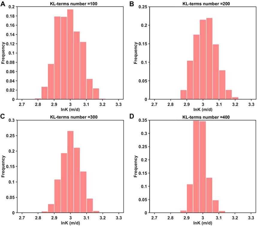
FIGURE 3. Frequency charts for different lnK ranges with various KL-terms numbers.

Figures 2, 3 reveal the spatial randomness and statistical characteristics (proportion of area) exhibited by sample means. In Figure 2, it is evident that when the KL-terms number is 100 and 200, the light lime region (values: 2.95–3.00) and pale yellow region (values: 3.00–3.05) are noticeably smaller compared to the cases with higher KL-terms (300, 400). In the case of the maximum KL terms (Figure 2D), there is the largest proportion of area around the mean (value: 2.95–3.05). For larger KL terms (in Figure 3), there is a greater proportion of area around the mean (value: 2.95–3.05).

Figure 4 reveal the spatial randomness exhibited by sample variances. Figure 4 illustrates that when the KL-terms number is 100, there is a significant deviation from the expected value of 1.0 (${\mathrm{\sigma }}_{lnK}^2=1.0$) in the statistical variance. However, as the number of KL-terms increases, the statistical variance tends to approach 1.0. In the case with KL-terms number = 400, the statistical variance predominantly concentrates in the range of 0.85–1.05, with a noticeable decrease in the occurrence of high and low variance regions.

FIGURE 4

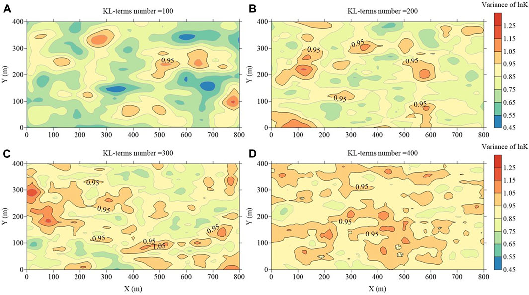
FIGURE 4. Statistical attribute (sample variance) with various KL-terms numbers.

In Figure 5, the dimensions of the red ellipse’s major and minor axes represent the correlation lengths in the x and y directions of the variogram (120 m and 60 m, respectively). In the subplots of Figure 5, a consistent pattern emerges: as the distance from the pumping well increases, the spatial correlation between sample points and the pumping well gradually decreases. Concurrently, with an increasing number of KL-terms, the covariance coefficients exhibit a more distinct unimodal trend, centered around the pumping well as the central peak.

FIGURE 5

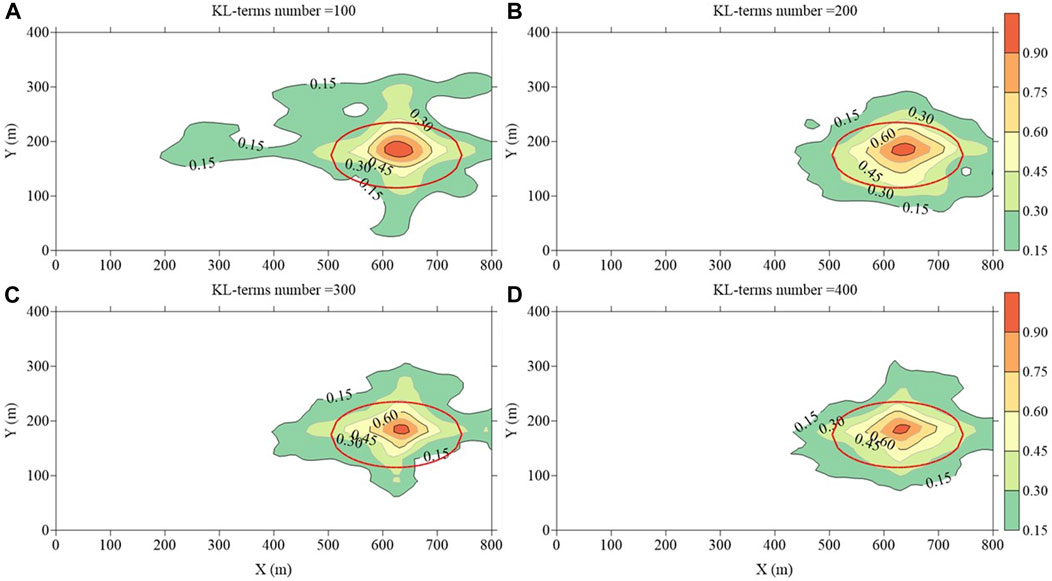
FIGURE 5. Statistical attribute (correlation coefficient) with various KL-terms numbers.

In a broader context, the statistical mean shown in Figure 2 remains relatively unaffected by the number of KL-terms. In contrast, the statistical attributes (variance and correlation coefficients), as depicted in Figures 4, 5, exhibit significant improvement with the utilization of 400 KL-terms, outperforming cases with fewer KL-terms. Notably, the sampling performance with 100 KL-terms falls short of expectations.

4.2 Stochastic simulation of WCZs

Expanding on the stochastic K-field obtained in Section 4.1, this section utilizes MODPATH for stochastic simulation of WCZs. It discusses the following aspects: (1) deterministic WCZs versus stochastic model WCZs; (2) probabilistic WCZs map; (3) the impact of the number of stochastic realizations. The scenario is set as follows: (a) Deterministic model: a homogeneous aquifer has a constant hydraulic conductivity of 20.08 m/d (i.e., lnK = 3.0); (b) Stochastic model: Within the stochastic model, Monte Carlo simulations are independently conducted with 10, 50, 100, 200, 300, and 400 times (KL-terms number = 400).

Figure 6 depicts the deterministic WCZs along with four random realizations (simulations) of K-field and their corresponding WCZs (100-day backward tracking). Contrasted with the WCZs obtained through the deterministic model (Figure 6A), it is evident that despite the mean ($\overline{lnK}=3.0\mathrm{m}/\mathrm{d}$) of the random K-fields being identical to the constant K value of the homogeneous K-field, there exist notable discrepancies in the resulting WCZs across various random realizations. The conventional deterministic model yields WCZs with considerable uncertainty.

FIGURE 6

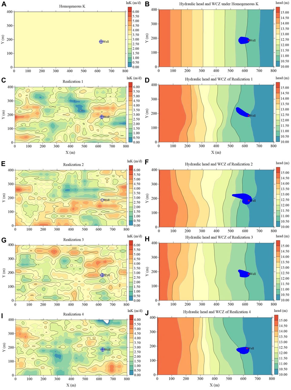
FIGURE 6. Various K-fields and the corresponding WCZs.

As shown in Table 1, the farthest points from pumping well exhibits significant variations in both distance and direction angle. Specifically, the farthest point corresponding to Figure 6F is located at NW66.04° from the pumping well, with a distance of 124.12 m, which is 1.79 times greater than that of the homogeneous K-field. Upon comparing the areas of WCZs in Figure 6, notable variations are evident. The maximum area, depicted in Figure 6F, is 6044 m², which is 1.88 times larger than the minimum area of 3217 m² illustrated in Figure 6H. Consequently, constructing protective zones for pumping wells based on such deterministic methodologies carries a substantial element of risk.

TABLE 1

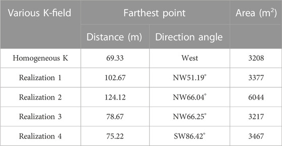
TABLE 1. The geometric features of WCZs with various K-fields.

As previously mentioned, the WCZs corresponding to various K-fields exhibit distinct patterns. With the limitations of available site data, individual K-fields introduce significant uncertainty when determining WCZs. Recognizing that uncertainty can be effectively conveyed through probability values, it is rational to consider the adopting of probabilistic maps for the determination of WCZs.

Given N random K-fields, the process involves determining whether each grid cell on the site is encompassed by backward tracking pathlines for each respective K-field. For grid points falling within the pathlines, they are denoted as 1 using m(i,j); conversely, for points not within the pathlines, they are denoted as 0. Subsequently, averaging these values yields the probability values representing the likelihood of grid points within the site being situated in the WCZs of the pumping wells.

$M\left(i,j\right)=\frac{1}{N}{\displaystyle \sum _{l=1}^N}m\left(i,j\right),(8)$

Further investigation delves into the impact of the number of stochastic simulations on the probabilistic WCZs map. In Figure 7 (100-day backward tracking), with a fixed number of KL-terms number (400), the subfigures labelled (a), (b), (c), (d), (e) and (f) correspond to stochastic simulation numbers of 10, 50, 100, 200, 300, and 400, respectively.

FIGURE 7

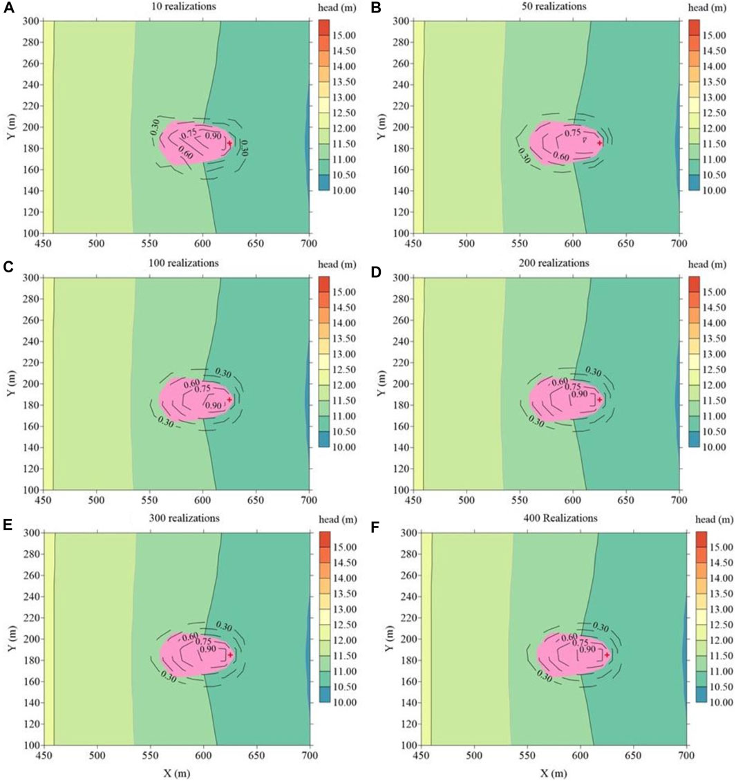
FIGURE 7. Probabilistic WCZs map based on different number of realizations in the stochastic simulations.

From the sequence of probabilistic WCZs maps, the following observations can be discerned: (1) The WCZs derived from the deterministic model (constant K) largely predominantly encompasses areas with a risk probability exceeding 60%. However, once the WCZs of pumping wells intersects with regions having a risk probability below 60%, relying solely on deterministically derived WCZs may lead to ineffectual decisions. (2) With an increasing number of realizations in the stochastic simulations, the probabilistic WCZ map demonstrates a gradual convergence pattern. When the number of stochastic simulations reaches 200 (as shown in Figure 7D), the degree of variation diminishes significantly, rendering the disparities from Figure 6F practically negligible.

4.3 Impact of strong heterogeneity level on WCZs

Based on the results in Section 4.1 and 4.2, it becomes evident that an increased number of KL-terms yields more effective stochastic modeling results. For the case of moderate heterogeneity, as detailed in Section 4.1 and 4.2, employing KL-terms number of 400 is adequate to preserve 93.49% of the total variance inherent in the K-field. In the case characterized by strong heterogeneity, the calculations derived from equation (4) indicate that, with KL-terms numbers of 400 and 800, they can preserve 88.76% and 95.16% of the total variance within the K-field, respectively.

Figure 8 illustrates the statistical attributes of different KL-terms numbers in the case of strong heterogeneity. Within this context, subfigures labelled (a), (c), and (e) depict sample means, sample variances, and correlation coefficients under KL-terms number of 400, and subfigures labelled (b), (d), and (f) describe sample means, sample variances, and correlation coefficients under KL-terms number of 800.

FIGURE 8

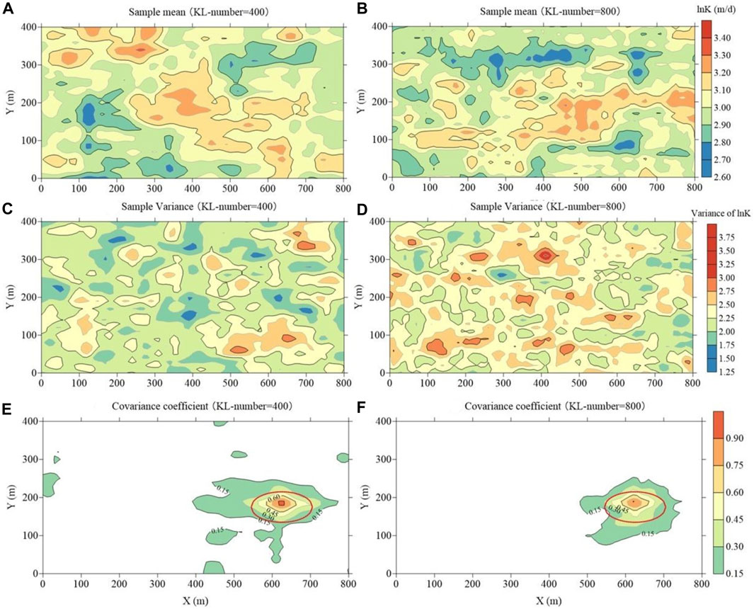
FIGURE 8. Statistical characteristics for different KL-terms numbers in the case of strong heterogeneity (Left: 400 KL-terms; Right: 800 KL-terms).

For two different levels of heterogeneity, in Figure 8A, the light lime region (values: 2.90–3.00) and pale yellow region (values: 3.00–3.10) appear notably smaller compared to the cases in Figure 2D with the same KL-terms number (=400). The statistical variance (in Figure 8C, Figure 4D) and correlation coefficient (in Figure 8E, Figure 5D) exhibit similar trends, indicating that under stronger heterogeneity, a greater number of KL-terms are required to characterize sufficient uncertainty.

Comparing Figures 8A, B for KL-terms numbers 400 and 800, the sample means are closely comparable, with Figure 8B slightly superior. Transitioning to Figures 8C, D, it is evident that when the KL-terms number is 400, the pale yellow region (values: 2.25–2.50) and light copper region (values: 2.50–2.75) are noticeably smaller compared to the cases with higher KL-terms (800). Figures 8E, F highlights a discernible trend where the spatial correlation between sample points and the pumping well gradually attenuates as the distance increases. Figure 8F’s correlation coefficients are more robust. Additionally, with the increase in the number of KL-terms from 400 to 800, a discernible decrease is observed in the extent of correlation coefficients exceeding 0.15 within the region outside the red ellipse.

These findings indicate that insufficient KL-terms may result in an incomplete characterization of the K-field, particularly in terms of variance and correlation coefficients. Even with an extensive number of Monte Carlo simulations, obtaining precise results may prove challenging as the generated K-fields cannot accurately reflect the spatial variability of the site’s permeability.

Figure 9 depicts probabilistic WCZs maps generated using varying numbers of stochastic simulations, applied to two distinct heterogeneous conditions. In these subfigures, the left column corresponds to the case of moderate heterogeneity (KL-terms number = 400), while the right column corresponds to the case of strong heterogeneity (KL-terms number = 800). From Figure 9, it can be observed that as the number of stochastic simulations increases, the probabilistic WCZs maps progressively display a tendency toward convergence. However, in the case of moderate heterogeneity, 200 simulations are required to attain this convergence. In contrast, for the case of strong heterogeneity, even with an increased number of KL-terms, a greater number of stochastic simulations (400 realizations) are still essential to achieve a convergent probabilistic WCZs map. It can be anticipated that using a lower number of KL-terms might lead to inadequate preservation of total variance and also impose a heightened demand for a greater number of stochastic simulations.

FIGURE 9

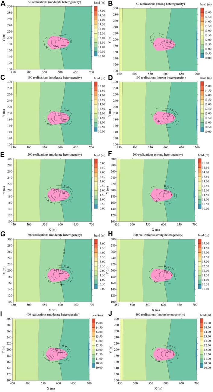
FIGURE 9. Probabilistic WCZ map based on different number of stochastic simulations (Left: moderate heterogeneity; Right: strong heterogeneity).

5 Conclusion

1) We employed a combination of the Karhunen-Loève Expansion (KLE) and Monte Carlo stochastic simulation method to delineate the probabilistic WCZ map in heterogeneous aquifers. For heterogeneous aquifers, the Monte Carlo stochastic simulation method proves effective in assessing WCZs while considering uncertainties. Furthermore, as an efficient Principal Component Analysis (PCA) method, the KLE method was adopted to reduce the dimensionality of hydraulic conductivity fields.

2) Compared to the WCZ obtained through the deterministic model, there are significant variations in the resulting WCZs for different random realizations. The conventional deterministic model yields deterministic WCZs with substantial uncertainty.

3) With the increasing KL-terms number, there is a noticeable improvement in the statistical characteristics of the samples. In Section 4.1, the statistical characteristics achieved with 400 KL-terms outperform cases with fewer KL-terms. Furthermore, the sampling performance for 100 KL-terms is unsatisfactory.

4) In comparison to the case of moderate heterogeneity, for the scenario of strong heterogeneity, a greater number of KL-terms (800 KL-terms) and a higher number of stochastic simulations (400 realizations) are required to achieve a convergent probabilistic WCZ map.

Data availability statement

Data and python codes of this study are available from the corresponding author on reasonable request (jiangsimin@tongji.edu.cn).

Author contributions

WG: Formal Analysis, Writing–original draft. GS: Conceptualization, Funding acquisition, Writing–review and editing. TZ: Formal Analysis, Methodology, Writing–review and editing. SJ: Methodology, Writing–review and editing.

Funding

The author(s) declare financial support was received for the research, authorship, and/or publication of this article. This work was supported by the Geological Exploration Project funded by Department of Natural Resources of Shandong Province [Lu Di Huan (2018) 06], and Scientific and Technological Innovation Team Project of Shandong Province Geo-mineral Engineering Exploration Institute (2022JBGS801-17).

Conflict of interest

The authors declare that the research was conducted in the absence of any commercial or financial relationships that could be construed as a potential conflict of interest.

Publisher’s note

All claims expressed in this article are solely those of the authors and do not necessarily represent those of their affiliated organizations, or those of the publisher, the editors and the reviewers. Any product that may be evaluated in this article, or claim that may be made by its manufacturer, is not guaranteed or endorsed by the publisher.

References

Bakker, M., Post, V., Langevin, C. D., Hughes, J. D., White, J. T., Starn, J., et al. (2016). Scripting MODFLOW model development using Python and FloPy. Groundwater 54 (5), 733–739. doi:10.1111/gwat.12413

PubMed Abstract | CrossRef Full Text | Google Scholar

Barry, F., Ophori, D., Hoffman, J., and Canace, R. (2009). Groundwater flow and capture zone analysis of the central passaic river basin, New Jersey. Environ. Geol. 56, 1593–1603. doi:10.1007/s00254-008-1257-5

CrossRef Full Text | Google Scholar

Christ, J. A., and Goltz, M. N. (2002). Hydraulic containment: analytical and semi-analytical models for capture zone curve delineation. J. Hydrology 262 (1-4), 224–244. doi:10.1016/s0022-1694(02)00026-4

CrossRef Full Text | Google Scholar

Ding, Y., Li, T., Zhang, D., and Zhang, P. (2008). Adaptive Stroud stochastic collocation method for flow in random porous media via Karhunen-Loeve expansion. Commun. Comp. Phys 4 (1), 102–123.

Google Scholar

EPA (1994). Handbook: ground water and wellhead protection. Washington, DC: Office of Research and Development, Office of Water.

Google Scholar

Fienen, M. N., Luo, J., and Kitanidis, P. K. (2005). Semi-analytical homogeneous anisotropic capture zone delineation. J. Hydrology 312 (1-4), 39–50. doi:10.1016/j.jhydrol.2005.02.008

CrossRef Full Text | Google Scholar

Frind, E. O., and Molson, J. W. (2018). Issues and options in the delineation of well capture zones under uncertainty. Groundwater 56 (3), 366–376. doi:10.1111/gwat.12644

CrossRef Full Text | Google Scholar

Harbaugh, A. W., Banta, E. R., Hill, M. C., and McDonald, M. G. (2000). Modflow-2000, the u. S. Geological survey modular ground-water model-user guide to modularization concepts and the ground-water flow process. United States: USGS.

Google Scholar

Haßler, S. K., Lark, R. M., Milne, A. E., and Elsenbeer, H. (2011). Exploring the variation in soil saturated hydraulic conductivity under a tropical rainforest using the wavelet transform. Eur. J. Soil Sci. 62 (6), 891–901. doi:10.1111/j.1365-2389.2011.01400.x

CrossRef Full Text | Google Scholar

Hunt, R. J., Steuer, J. J., Mansor, M. T. C., and Bullen, T. D. (2001). Delineating a recharge area for a spring using numerical modeling, Monte Carlo techniques, and geochemical investigation. Groundwater 39 (5), 702–712. doi:10.1111/j.1745-6584.2001.tb02360.x

PubMed Abstract | CrossRef Full Text | Google Scholar

Jiang, S., Liu, J., Xia, X., Wang, Z., Cheng, L., and Li, X. (2021). Simultaneous identification of contaminant sources and hydraulic conductivity field by combining geostatistics method with self-organizing maps algorithm. J. Contam. Hydrol. 241, 103815. doi:10.1016/j.jconhyd.2021.103815

PubMed Abstract | CrossRef Full Text | Google Scholar

Jiang, Y., Zhang, J., Zhu, Y., Du, Q., Teng, Y., and Zhai, Y. (2019). Design and optimization of a fully-penetrating riverbank filtration well scheme at a fully-penetrating river based on analytical methods. Water 11 (3), 418. doi:10.3390/w11030418

CrossRef Full Text | Google Scholar

Lu, C., Qin, W., Zhao, G., Zhang, Y., and Wang, W. (2017). Better-fitted probability of hydraulic conductivity for a silty clay site and its effects on solute transport. Water 9 (7), 466. doi:10.3390/w9070466

CrossRef Full Text | Google Scholar

Moeck, C., Molson, J., and Schirmer, M. (2020). Pathline density distributions in a null-space Monte Carlo approach to assess groundwater pathways. Groundwater 58 (2), 189–207. doi:10.1111/gwat.12900

CrossRef Full Text | Google Scholar

Mohebbi Tafreshi, A., Nakhaei, M., Lashkari, M., and Mohebbi Tafreshi, G. (2019). Determination of the travel time and path of pollution in Iranshahr aquifer by particle-tracking model. SN Appl. Sci. 1 (12), 1616. doi:10.1007/s42452-019-1596-8

CrossRef Full Text | Google Scholar

Nalarajan, N. A., Govindarajan, S. K., and Nambi, I. M. (2019). Numerical modeling on flow of groundwater energies in transient well capture zones. Environ. Earth Sci. 78, 142–214. doi:10.1007/s12665-019-8176-5

CrossRef Full Text | Google Scholar

Patriarche, D., Castro, M. C., and Goovaerts, P. (2005). Estimating regional hydraulic conductivity fields—a comparative study of geostatistical methods. Math. Geol. 37, 587–613. doi:10.1007/s11004-005-7308-5

CrossRef Full Text | Google Scholar

Pebesma, E. J., and Wesseling, C. G. (1998). Gstat: a program for geostatistical modelling, prediction and simulation. Comput. Geosci-Uk 24 (1), 17–31. doi:10.1016/s0098-3004(97)00082-4

CrossRef Full Text | Google Scholar

Pollock, D. W. (2016). User guide for MODPATH Version 7—a particle-tracking model for MODFLOW. United States: US Geological Survey.

Google Scholar

Qiao, X., Li, G., Li, Y., and Liu, K. (2015). Influences of heterogeneity on three-dimensional groundwater flow simulation and wellhead protection area delineation in karst groundwater system, Taiyuan City, Northern China. Environ. Earth Sci. 73, 6705–6717. doi:10.1007/s12665-015-4031-5

CrossRef Full Text | Google Scholar

Robin, M. J. L., Gutjahr, A. L., Sudicky, E. A., and Wilson, J. L. (1993). Cross-correlated random field generation with the direct Fourier transform method. Water Resour. Res. 29 (7), 2385–2397. doi:10.1029/93wr00386

CrossRef Full Text | Google Scholar

Rock, G., and Kupfersberger, H. (2002). Numerical delineation of transient capture zones. J. Hydrology 269 (3-4), 134–149. doi:10.1016/s0022-1694(02)00238-x

CrossRef Full Text | Google Scholar

Shan, C. (1999). An analytical solution for the capture zone of two arbitrarily located wells. J. Hydrology 222 (1-4), 123–128. doi:10.1016/s0022-1694(99)00101-8

CrossRef Full Text | Google Scholar

Turcke, M., and Kueper, B. (1996). Geostatistical analysis of the Borden aquifer hydraulic conductivity field. J. Hydrology 178 (1-4), 223–240. doi:10.1016/0022-1694(95)02805-6

CrossRef Full Text | Google Scholar

Xue, L., Dai, C., Wu, Y., and Wang, L. (2018). Towards improving the efficiency of Bayesian model averaging analysis for flow in porous media via the probabilistic collocation method. Water 10 (4), 412. doi:10.3390/w10040412

CrossRef Full Text | Google Scholar

Zhang, D., and Lu, Z. (2004). An efficient, high-order perturbation approach for flow in random porous media via Karhunen–Loeve and polynomial expansions. J. Comput. Phys. 194 (2), 773–794. doi:10.1016/j.jcp.2003.09.015

CrossRef Full Text | Google Scholar

Zhang, J., Lin, G., Li, W., Wu, L., and Zeng, L. (2018). An iterative local updating ensemble smoother for estimation and uncertainty assessment of hydrologic model parameters with multimodal distributions. Water Resour. Res. 54 (3), 1716–1733. doi:10.1002/2017wr020906

CrossRef Full Text | Google Scholar

Zhu, Y., Zhai, Y., Du, Q., Teng, Y., Wang, J., and Yang, G. (2019). The impact of well drawdowns on the mixing process of river water and groundwater and water quality in a riverside well field, Northeast China. Hydrol. Process. 33 (6), 945–961. doi:10.1002/hyp.13376

CrossRef Full Text | Google Scholar