Intelligent reconstruction for spatially irregular seismic data by combining compressed sensing with deep learning

Data reconstruction is the most essential step in seismic data processing. Although the compressed sensing (CS) theory breaks through the Nyquist sampling theorem, we previously proved that the CS-based reconstruction of spatially irregular seismic data could not fully meet the theoretical requirements, resulting in low reconstruction accuracy. Although deep learning (DL) has great potential in mining features from data and accelerating the process, it faces challenges in earth science such as limited labels and poor generalizability. To improve the generalizability of deep neural network (DNN) in reconstructing seismic data in the actual situation of limited labeling, this paper proposes a method called CSDNN that combines model-driven CS and data-driven DNN to reconstruct the spatially irregular seismic data. By physically constraining neural networks, this method increases the generalizability of the network and improves the insufficient reconstruction caused by the inability to sample randomly in the whole data definition domain. Experiments on the synthetic and field seismic data show that the CSDNN reconstruction method achieves better performance compared with the conventional CS method and DNN method, including those with low sampling rates, which verifies the feasibility, effectiveness and generalizability of this approach.

1 Introduction

With the gradually complex targets of petroleum exploration and development, as well as the promotion of the wide-band, wide-azimuth and high-density seismic acquisition technologies, research has been increasingly focusing on efficient and low-cost acquisition technology. In addition, due to the acquisition environment and economic factors constrains in exploration, the obtained spatially irregular and incomplete seismic data usually cannot satisfy the Nyquist–Shannon sampling theorem. Such missing trace data seriously affects the subsequent seismic data processing, which in turn impairs the reliability of the final interpretation. Thus, effective reconstruction is meaningful for seismic data processing to accurately depict complex geological structures and provide more effective instructions and assistance for petroleum exploration.

Currently, the major ap proaches used to reconstruct spatially irregularly distributed seismic data include model-driven methods based on the knowledge of mathematical equations or time-space variation characteristics, and data-driven methods based on deep learning (DL) from big data.

Model-driven methods mainly encompass predictive filtering methods (Spitz, 1991), wave equation methods (Ronen, 1987; Trad, 2003; Zhao et al., 2021), sparse-transform methods (Zwartjes and Gisolf, 2006; Herrmann and Hennenfent, 2008; Mousavi et al., 2016) and low-rank approximation methods (Oropeza and Sacchi, 2011; Wang et al., 2017; Innocent Oboué et al., 2021). Among them, the sparse-transform and low-rank promotion methods are closely related to the compressed sensing (CS) method (Donoho, 2006a), which treats reconstruction as an underdetermined linear inversion problem solved using the sparsity constraint in the transform domain. Compared with the method based on predictive filtering, the CS-based method involves the sparsity and the spatiotemporal variation characteristics of data, which also does not require prior knowledge of the geological model needed by wave equation methods.

The existing research around the CS method mainly focuses on sparse transformation and reconstruction algorithms, with sparse transformations such as Fourier (Naghizadeh and Innanen, 2011), Curvelet (Hennenfent et al., 2010), Dreamlet (Wang et al., 2015), Radon (Ibrahim et al., 2018), Framelet (Pan et al., 2023), etc. To solve sparse optimization problems, regularization algorithms are commonly used, such as ${\mathrm{L}}_0$ norm (Chen et al., 2013), ${\mathrm{L}}_1$ norm (Yin et al., 2015), non-convex ${\mathrm{L}}_{\mathrm{P}}$ norm (Zhong et al., 2015), etc. According to the CS theory, the data sparsity domain and the acquisition matrix must have the same definition domain. Seismic data controlled by second-order partial differential equation has sparsity in the time-space domain, but spatially irregular data is obtained by compressed acquisition only in spatial domain, so the compressed acquisition domain is inconsistent with the data sparsity domain used in reconstruction. In other words, there is a theoretical defect in the application process, hence the reconstruction of the CS-based method for spatially irregular seismic data is difficult to meet the production requirements, especially for low sampling rates.

In the past decade, data-driven artificial intelligence (AI) has been highly valued in seismic exploration, and the rise of DL has greatly promoted the research of intelligent seismic data processing, inversion, interpretation, and other fields. For seismic data reconstruction, various deep neural network (DNN) structures have been increasingly used for this research topic, such as convolutional neural networks (CNN), ResNet (Wang et al., 2019), 3D denoising convolutional neural network (3-D-DnCNN) (Liu et al., 2020), U-Net (Chai et al., 2020), prediction-error filters network (PEFNet) ((Fang et al., 2021a)), multi-dimensional adversarial GAN (MDA GAN) (Dou et al., 2023), etc. The deepening and complexity of the network structure not only increases the amount of computation but also brings gradient instability, network degradation, and the model being over-parameterized; it becomes difficult for the trained model to stably generalize to new missing data with different distributions. Moreover, most of the existing DL-based methods refer to the concept of computer vision completion, and the difference between image processing and seismic data reconstruction should be considered in further research, that is, incorporating richer characteristics of the seismic data (Luo et al., 2023).

During the research process, we can see that it has been difficult to achieve the goal of AI seismic exploration with a single route or paradigm. Wu et al. (Wu et al., 2023) concluded that domain knowledge constraints can be applied to deep neural networks to improve those with weak generalization ability, low interpretability and poor physical consistency, such as physics-driven intelligent seismic processing (Pham and Li, 2022), impedance inversion (Yuan et al., 2022), porosity prediction (Sang et al., 2023), designing prior-constraint network architectures for seismic waveform inversion (Sun et al., 2020) and exploring the physics-informed neural network (PINN) for solving geophysical forward modeling (Song and Wang, 2023). From these studies, we conclude that a more reasonable direction to deal with reconstruction problems can be the combination of data-driven model and mechanism model.

In light of the shortcomings of conventional DL seismic data reconstruction, we propose a strategy for reconstructing spatially irregular data by integrating CS and DL methodologies, called CSDNN. First, we prove the theoretical flaw in the CS-based reconstruction of spatially irregularly acquired seismic data. Second, we present the DL method to reconstruct seismic data with DnCNN and analyze its pros and cons. Thirdly, we combine data-driven and model-driven models and refer to the sequential strategy used in the joint inversion of multiple geophysical data to establish the optimal objective function, and adopt a step-by-step optimization algorithm to achieve high-precision and high signal-to-noise ratio (SNR) reestablishment. Numerical experiments demonstrate the efficiency and the improvement in the generalizability of the suggested strategy, even for low-sampling-rate data.

2 Methodology

2.1 Reconstruction using CS

2.1.1 Irregular seismic data acquisition based on CS

Seismic data acquisition is conducted by adhering to the spatiotemporal variation law of the wavefield $u\left(x,y,t;x_s,y_s\right)$ and utilizing the Nyquist–Shannon sampling theorem to regularly perform equidistant discretization in the five dimensions of $x$, $y$, $t$, $x_s$ and ${\mathrm{y}}_{\mathrm{s}}$, as shown in (Eq. 1):

$u\left(x_i,y_j,t_k{;x}_{sl},y_{sm}\right)={\displaystyle \sum _{m=0}^{Ms-1}}{\displaystyle \sum _{l=0}^{Ls-1}}{\displaystyle \sum _{k=0}^{K-1}}{\displaystyle \sum _{j=0}^{J-1}}{\displaystyle \sum _{i=0}^{I-1}}\delta \left(y-y_j\right)\delta \left(x-x_i\right)\times \delta \left(t-t_k\right)\delta \left(y_s-y_{sm}\right)\delta \left(x_s-x_{sl}\right)u\left(x,y,t{;x}_s,y_s\right),(1)$

where $u\left(x_i,y_j,t_k{;x}_{sl},y_{sm}\right)$ represents the obtained spatiotemporal domain discretized data, $x_i=i\Delta x$, $y_j=j\Delta y,t_k=k\Delta t,x_{sl}=l\Delta x_s$ and $y_{sm}=m\Delta y_s$. In this context, $x$ and $y$ denote the coordinates of the receiving points; $x_s$ and ${\mathrm{y}}_{\mathrm{s}}$ denote the coordinates of the shot points, and $t$ is the number of time variable. $Ms$, $Ls$, $K$, $J$ and $I$ represent the number of shot lines, the number of shots per shot line, the number of time samples, the number of receiver lines, and the number of receivers per line, respectively. $\delta \left(f\right)$ is the Dirac delta function (Piela, 2014).

The CS theory states that if the signal $\mathit{u}$ is sparse or sparse in a transform domain, it can be projected from the high-dimensional space to the low-dimensional space through the sampling matrix $\mathit{W}$, which is uncorrelated with the basis function of sparse transform, to obtain an observed signal $\mathit{d}$ that is much smaller than the original signal length. Then, the original signal $\mathit{u}$ can be recovered by the reconstruction algorithm (Donoho, 2006b; Candès et al., 2006). If incomplete data $\mathit{d}$ can reconstruct complete data $\mathit{u}$, then $\mathit{d}$ can be regarded as the compressed sample data of $\mathit{u}$, where the linear mapping of $\mathit{d}$ to $\mathit{u}$ is formulated as follows:

${\mathit{d}}^{M\times 1}{=\mathit{W}}^{M\times N}{\mathit{u}}^{N\times 1},(2)$

where $M$ and $N$ denote the number of irregular and regular sampling points, respectively, with $M\ll N$ ; the incomplete data $\mathit{d}\in {\mathbb{R}}^{\mathrm{M}\times 1}$ can be regarded as an $M\times 1$ column matrix, where $\mathbb{R}$ means the field of real numbers; the complete data $\mathit{u}\in {\mathbb{R}}^{N\times 1}$ is a regular equidistant vector with sparsity, and $\mathit{u}$ also can be regarded as an $N\times 1$ column matrix; $\mathit{W}\in {\mathbb{R}}^{M\times N}$ is a random sampling matrix composed of 0 and 1, and there are $M$ elements with a value of 1. If the complete data $\mathit{u}$ comprises the regular discrete data sequence $u\left(x_i,y_j,t_k{;x}_{sl},y_{sm}\right)$ in (Eq. 1), then the compressed sampling of $\mathit{d}$ can break the sampling interval limitation in the Nyquist theorem, where $N=Ms\times Ls\times K\times J\times I$, and $\mathit{W}$ should have the same definition domain as $\mathit{u}$.

Although high-dimensional data can make better use of the spatial correlation, for a theoretically concise demonstration, we simplify the problem to 2D seismic data but the conclusions obtained can be extended to 5D. By sampling $u\left(x_i,y_j,t_k{;x}_{sl},y_{sm}\right)$ regularly in the 2D spatiotemporal domain, the discrete sampling Equation 1 can be abbreviated as:

$u\left(x_i,t_k,x_s\right)=\sum _{k=0}^{K-1}\sum _{i=0}^{I-1}\delta \left(t-t_k\right)\delta \left(x-x_i\right)u\left(x,t,x_s\right).(3)$

The CS theory provides a conceptual foundation for the sparse acquisition of seismic data, which could greatly improve efficiency and reduce costs in fieldwork. According to the CS-based sparse sampling in Eq. 2) and ignoring the shot point coordinates $x_s$ in (Eq. 3), the irregular sampling for 2D seismic data in the definition domain can be written as:

$u\left(x_{ri},t_{rk}\right)=\sum _{r=0}^{N-1}\delta \left(t_{rk}-{\mathrm{t}}_k\right)\delta \left(x_{ri}-x_i\right)u\left(x_i,t_k\right),(4)$

where $\left(x_{ri},t_{rk}\right)$ represents the spatiotemporal location of $M$ randomly selected sampling points $\left(x_i,t_k\right)$ from $N=I\times K$ regularly equally spaced sampling points of $u\left(x_i,t_k\right)$. Among the $N$ elements in each row of the sampling matrix $\mathit{W}$, the value is 1 only in one random position while all other element values are zero, so $\mathit{W}$ is a random sampling matrix in the whole data definition domain. Compared with the Nyquist acquisition (Eq. 1), compressed acquisition (Eq. 4) can greatly reduce the amount of collected data. However, the sampling points are randomly and irregularly distributed, so compressed acquisition (Eq. 4) neither reduces the cost (except for data storage and transmission) nor improves the acquisition efficiency.

In seismic exploration, three main factors cause the acquired data to be spatially irregular. Firstly, the complicated exploration environment and human geographic factors in the work area lead to irregular distribution of shot and receiver positions. Secondly, the recording geometry is affected by nature resulting in changes. For example, due to waves, currents and tides in the ocean, the receiver points deviate from the preset position. Thirdly, when applying CS acquisition techniques while reducing the cost and improve the acquisition efficiency, irregular sparse sampling points are only randomly collected in the spatial dimensions of the data, and Nyquist sampling is followed in the temporal dimension (only this case is considered in this paper). Then, the high-efficiency acquisition of temporally regular and spatially irregular sampling can be written as:

$u\left(x_{ri},t_k\right)=\sum _{k=0}^{K-1}\sum _{ri=0}^{Ir-1}\delta \left(t_k-{\mathrm{t}}_k\right)\delta \left(x_{ri}-x_i\right)u\left(x_i,t_k\right)=\sum _{ri=0}^{Ir-1}\delta \left(x_{ri}-x_i\right)u\left(x_i,t_k\right),(5)$

where $x_{ri}$ denotes the location of $Ir$ traces randomly selected from $I$ regular equidistant seismic traces $x_i$. For the sampling matrix $\mathit{W}$, the $M$ elements with value 1 in $\mathit{W}$ correspond to the locations of $K$ regular time sampling points of $Ir$ traces randomly selected from $I$ regular distributed seismic traces, thus $\mathit{W}$ in (Eq. 5) is not random sampling in the whole definitional domain of data. Clearly, in the acquisition of spatially irregular data, random sampling in the time dimension can decrease the number of time samples but cannot reduce the total time or the time cost. Therefore, the CS acquisition method is not used in the time dimension. Compared with (Eq. 1), compressed acquisition (Eq. 5) greatly reduces the number of seismic traces or the same number of traces can cover a wider area, eventually lowering the cost and increasing the acquisition efficiency.

For Eq. 5, it can be seen that the acquisition of spatially irregular seismic data is not compressive sampling that fully satisfies the CS theory, and the number of shot-detection points is far less than the conventional regular shot-detection grid. Therefore, this is a high-efficiency and low-cost acquisition method based on the concept of CS (data sparsity and irregular sampling).

2.1.2 Theoretical defect of CS-based reconstruction for spatially irregular seismic data

It is well known that CS is not only a high-efficiency signal sampling method but also a high-resolution data reconstruction method. The three important prerequisites for CS include: (i) the complete signal satisfies sparsity or compressibility; (ii) the sampling matrix should be a random matrix in the data definition domain, which is independent of the signal; and (iii) a suitable high-precision reconstruction algorithm that promotes sparsity.

The CS theory-based reconstruction strategy is the process that satisfies all of the above three conditions, and then recovers the original data $\mathit{u}$ from the sampling matrix $\mathit{W}$ and the observation data $\mathit{d}$ by finding the minimum norm solution of the underdetermined system of equations, as follows:

$\mathrm{O}\left(\mathbf{c}\right)=\min \left({‖\mathbf{d}-\text{Sc}‖}_2^2\right),s.t.{‖\mathit{c}‖}_1\le \sigma ,(6)$

where $\mathrm{O}\left(\mathbf{c}\right)$ denotes the optimization objective function with $\mathbf{c}$ as a variable; c is the sparse transform coefficient of data $\mathit{u}$ to be reconstructed, with $\mathit{c}=\mathrm{\Phi }\mathit{u}$, $\mathit{u}={\mathrm{\Phi }}^{-1}\mathit{c}$; $\mathrm{\Phi }$ and ${\mathrm{\Phi }}^{-1}$ represent the sparse transformation and inverse transformation applicable to $\mathit{u}$, respectively; $\mathbf{S}$ denotes the sensing matrix, with $\mathit{S}=\mathit{W}{\mathrm{\Phi }}^{-1}$ ; $\sigma$ is a quantity that measures the sparsity of $\mathit{c}$.

The constrained optimization problem in (Eq. 6) can also be converted into the following unconstrained optimization problem:

$O\left(\mathit{u}\right)=\min \left({‖\mathit{d}-\mathit{W}\mathit{u}‖}_2^2+\lambda {‖\mathrm{\Phi }\mathit{u}‖}_1\right),(7)$

where $\lambda$ is a regularization parameter. There are many algorithms for solving optimization problems (Eqs. 6, 7). The common CS reconstruction algorithms have been applied in seismic data reconstruction, such as the Projection onto Convex Set (POCS) algorithm (Abma and Kabir, 2006), Iterative Soft Thresholding (IST) algorithm (Hennenfent et al., 2010) and Orthogonal Matching Pursuit (OMP) algorithm (Sun et al., 2018). Eqs. 6, 7 are recognized as model-driven methods for reconstruction because they are generated through the mathematical representation (Eq. 5) of seismic data and the prior knowledge of spatiotemporal variation (i.e., sparsity).

Due to the sampling matrix directly affecting the quality of the compressed information, certain constraints need to be met when constructing this matrix, such as null space, constrained equidistant properties and incoherence. However, in the CS-based reconstruction for spatially irregular seismic data, the sampling matrix $\mathit{W}$ in (Eq. 5) is irregularly random sampling only in the spatial dimension of seismic data but not in the time dimension, which does not satisfy the CS precondition that the sampling matrix should be random in the whole data domain. Therefore, there is a theoretical flaw in the CS-based reconstruction method commonly used in this case, making it difficult to obtain high SNR reconstruction, especially for data with low sampling rate.

Although the collection corresponding to (Eq. 4) satisfies the CS theoretical requirements, it cannot improve efficiency, or save time and economic cost in actual production. Therefore, we propose a pseudo-CS acquisition, that is, pseudo-spatiotemporally irregular acquisition, where the seismic traces are randomly sampled at the sampling rate $r_1$, then the extracted traces are randomly sampled in the spatiotemporal domain at the sampling rate $r_2$, so the total sampling rate is $r_1{r}_2$. We use a 2D synthetic seismic data $u_1$ with 512 traces, 512 samples in each trace, and a sampling interval of 2 ms as the complete data. Irregular sampling is performed in spatial ${\mathit{d}}_x$ (Figures 1A, D), pseudo-spatiotemporal ${\mathit{d}}_{pxt}$ (Figures 1G, J), and spatiotemporal domain ${\mathit{d}}_{xt}$ (Figures 1M, P). We abbreviate the sampling rate as SR. The SR of each sampling method is 30% (Figures 1A, G, M) and 50% (Figures 1D, J, P). Under the same SR, the number of points collected is consistent.

FIGURE 1

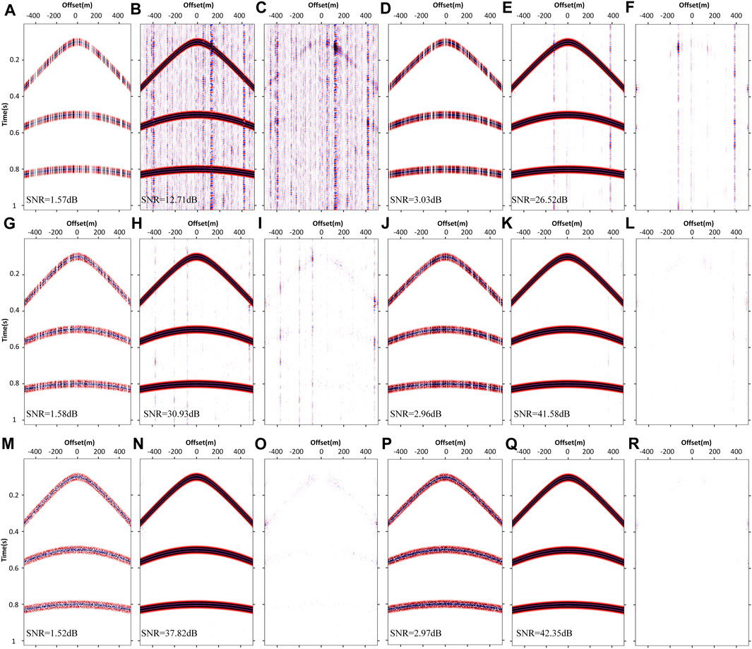
FIGURE 1. Irregularly sampled data and corresponding reconstructions and residuals for synthetic seismic data ${\mathit{u}}_{\mathbf{1}}$. (A) ${\mathit{d}}_{\mathit{x}}$ (SR = 30%); (B) ${\mathit{u}}_{\mathit{x}}$ of (A); (C) difference between ${\mathit{u}}_{\mathbf{1}}$ and (B); (D) ${\mathit{d}}_{\mathit{x}}$ (SR=50%); (E) ${\mathit{u}}_{\mathit{x}}$ of (D); (F) difference between ${\mathit{u}}_{\mathbf{1}}$ and (C); (G) ${\mathit{d}}_{\mathit{p}\mathit{x}\mathit{t}}$ (SR = 30%); (H) ${\mathit{u}}_{\mathit{x}}$ of (G); (I) difference between ${\mathit{u}}_{\mathbf{1}}$ and (H); (J) ${\mathit{d}}_{\mathit{p}\mathit{x}\mathit{t}}$ (SR = 50%); (K) ${\mathit{u}}_{\mathit{x}}$ of (J); (L) difference between ${\mathit{u}}_{\mathbf{1}}$ and (K); (M) ${\mathit{d}}_{\mathit{x}\mathit{t}}$ (SR = 30%); (N) ${\mathit{u}}_{\mathit{x}}$ of (M); (O) difference between ${\mathit{u}}_{\mathbf{1}}$ and (N); (P) ${\mathit{d}}_{\mathit{x}\mathit{t}}$ (SR = 50%); (Q) ${\mathit{u}}_{\mathit{x}}$ of (P); (R) difference between ${\mathit{u}}_{\mathbf{1}}$ and (O).

We take the discrete cosine transform (DCT) as the sparse transformation and use the IST algorithm to obtain the final CS reconstruction ${\mathit{u}}_x$, ${\mathit{u}}_{pxt}$ and ${\mathit{u}}_{xt}$, as shown in Figure 1. By comparison, the reconstruction result ${\mathit{u}}_{xt}$ is significantly better than ${\mathit{u}}_x$ and ${\mathit{u}}_{pxt}$ at each same SR. When the SR is lower, the deficiency of ${\mathit{u}}_x$ is more obvious, indicating that the CS-based spatially irregular reconstruction is acceptable when the SR is relatively high. This also explains the rationality of the current widely used spatially irregular CS in the study of seismic data reconstruction, but in the presence of the aforementioned theoretical defect, insufficient reconstruction would be obvious under a low SR. As a trade-off scheme between the acquisition efficiency and the randomness of the sampling matrix, the sampling points of pseudo-CS acquisition are carried out in the spatiotemporal domain of the collected traces. In Figure 1G, we set the SR of seismic traces to be consistent with the SR of the space-time, so that the total sampling rate is 30%, but the sampling matrix is closer to the randomness of whole data definition domain, and more traces are collected than Figure 1A. Figure 1H is obviously different from Figure 1B, which corroborates our reasoning and reflects the importance of the randomness in the data definition domain. Comparing the reconstruction of the three acquisition forms, we prove that irregular data will have better a CS reconstruction when it is closer to the randomness of the whole domain.

Although CS-based irregular spatiotemporal acquisition offers more accurate reconstruction, the efficiency and cost of acquisition cannot be improved in actual exploration. On the other hand, spatially irregular acquisition is effective and economical, but the reconstruction is poor especially under a low SR. Therefore, it is urgent to interpolate the irregular missing seismic trace with high precision and SNR.

2.2 Reconstruction by supervised learning

Reconstructing seismic data using traditional methods can be both computationally expensive and susceptible to various human factors. By utilizing supervised learning, the missing traces can be recovered by learning the mapping between input and label from a vast quantity of data. These data-driven approaches do not account for the irregularity, spatiotemporal variation or the impact of sparse transformation of seismic data. The DL-based seismic data reconstruction usually assumes that there is a nonlinear mapping relationship $Net$ between the known regular seismic data $\mathit{u}$ and its corresponding spatially irregular seismic data $\mathit{d}$, which can be represented by a DNN model as follows:

$\mathit{u}=Net\left(\mathit{d},\mathit{\theta }\right),(8)$

where $\mathit{\theta }$ represents the parameters that constitute the network.

We record the existing complete data as the label ${\mathit{u}}_{\mathit{l}\mathit{a}\mathit{b}}$ and the existing spatially irregular data as the training data $\mathit{d}$. The following optimization algorithm is usually solved to obtain the $\widehat{\mathit{\theta }}$ corresponding to the minimum of $\mathrm{O}\left(\mathit{\theta }\right)$:

$O\left(\mathit{\theta }\right)=\mathit{min}\left({‖Net\left(\mathit{d},\theta \right)-{\mathit{u}}_{lab}‖}_2^2\right).(9)$

Based on the trained parameters $\widehat{\mathit{\theta }}$, we take the spatially irregular data $\mathit{d}$ outside the training set to obtain the corresponding reconstruction $\widehat{\mathit{u}}$. This process is the generalization of (Eq. 9) and can be expressed in (Eq. 10):

$\widehat{\mathit{u}}=Net\left(\mathit{d},\widehat{\mathit{\theta }}\right).(10)$

The reconstruction performance of (Eq. 10) largely depends on the generalizability of the network model represented by $\widehat{\mathit{\theta }}$. Using the network model with excellent generalizability can better recover data; otherwise, it is difficult to guarantee the reconstruction in network promotion.

For DL training, we adopt the DnCNN architecture depicted in Figure 2, whose residual learning mode focuses the mapping connection on the distinction between labels and input data instead of directly learning the mapping between them. This network is simpler to optimize and effectively avoids the gradient dispersion problem during training because most of the residuals are small. The DnCNN comprises 17 convolutional layers, with the first layer consisting of convolution (Conv) and rectified linear unit (ReLU), the second through 16th layers consisting of Conv, Batch normalization (BN) and ReLU, and the 17th layer is a Conv.

FIGURE 2

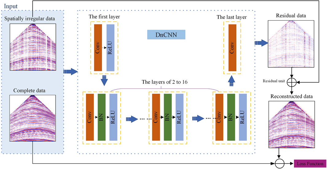
FIGURE 2. Architecture of DnCNN.

The benefits of DL-based methods, such as nonlinear mapping and automatic feature extraction, are valuable for reconstructing seismic data, while challenges persist such as limited training data sets, uncertainty and poor generalization. On the one hand, the spatial characteristics of seismic data learned by the network may have difficulty correctly interpolating in a large missing ratio; many studies only showed the reconstruction when fewer traces were missing ($\text{SR}$ more than 50%) (Fang et al., 2021b). On the other hand, the trained models may fail to generalize well on new samples with different distributions. In Wang’s DNN-based residual learning method for seismic reconstruction, as the feature disparity between the test field data and the training data set grows, the interpolation deviation becomes more obvious (Wang et al., 2019).

The application impact of DL-based method depends on the generalizability of the network, making it challenging to implement in actual production. The main determinants affecting the performance of network models include the network structure, the optimization algorithm, the size and feature diversity of the dataset used for training, the computer processing capability, etc. The following methods can be used to improve the network generalizability: (i) training more data with a wider range of features; (ii) modifying or reshaping the network architecture to incorporate mathematical and physical operators; (iii) adjusting the objective function by adding the constraints of the mathematical expression and prior knowledge about the data.

However, it is not easy to measure how much data is obtained with a larger number and higher diversity of characteristics, which may bring some practical difficulties. In terms of incorporating mathematical, physical and prior data knowledge into the goal function (Eq. 10), although some methods have been proposed recently and certain progress has been made, these are still in the process of exploration (Mousavi and Beroza, 2022). Such methods imply that under the condition of the limited training dataset, constructing a network with excellent generalizability is a difficult task, and this method also has challenges regarding research and application for the reconstruction of spatially irregular seismic data.

2.3 Data and model dual-driven seismic data reconstruction

In statistical learning theory, the complexity of hypothesis space $H$, which includes the set of all possible mapping relations of the learning algorithm, is a key factor to analyze the generalization ability of network models (Vapnik, 1999; Wu and Zhang, 2017). For common regression problems, the complexity of the mapping relationship between label and data is sometimes difficult to quantify and characterize. However, for seismic data reconstruction, the label is the complete seismic record, the input data is a spatially irregular seismic record, and labels and data are essentially the same kind of data, with the difference degree corresponding to the complexity of the relationship between them. Therefore, for fitting the desired mapping between $\mathit{u}$ and $\mathit{d}$ in (Eq. 8), reducing the difference between the two is equivalent to weakening the complexity of mapping relationship, thereby narrowing the dimension of hypothesis space. In this way, the learned parametric model can approximate the true model with greater probability, thus increasing the network generalization ability.

Moreover, the seismic record comprises spatiotemporal data that satisfies the wave equation; hence, the process of CS searching for suitable sparse transformation to obtain few coefficients to represent the data is actually controlled by mathematical physics, which is a kind of mode knowledge. Based on the above discussion, we propose a method for reconstructing the spatially irregular seismic data that combines CS and DL. Firstly, using CS for preliminary reconstruction to obtain the input data of DnCNN, we reduce the difference between $\mathit{u}$ and $\mathit{d}$ in the sample set and lower the complexity and nonlinearity of network training, which is carried out to enhance the generalization of the network model by incorporating prior knowledge into DL. Then, the reconstruction is carried out by data-driven iteration. We refer to this method as CSDNN for short, with its structure shown in Figure 3.

FIGURE 3

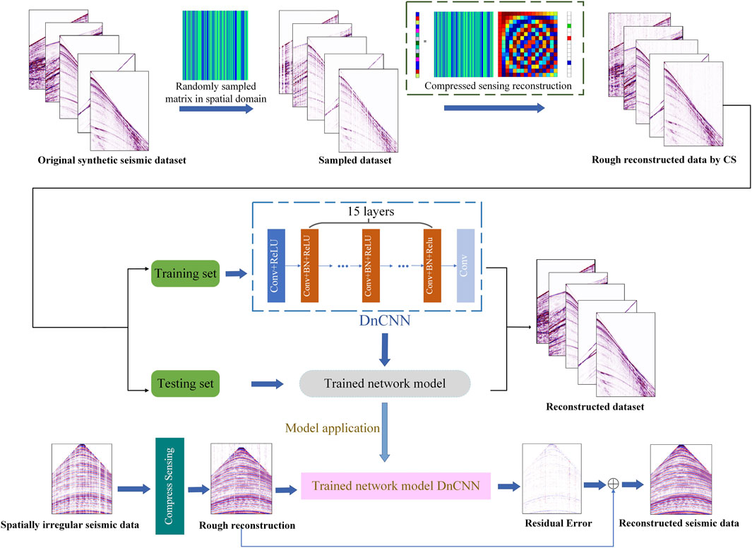
FIGURE 3. CSDNN: the proposed architecture for spatially irregular seismic data reconstruction.

In the training dataset, the spatially irregular seismic data $\mathit{d}$ is used as input data and the corresponding complete data ${\mathit{u}}_{lab}$ is used as the label. The objective function of our data and model dual-driven method CSDNN can be written as:

$O\left(\mathit{u},\mathit{\theta }\right)=\mathit{min}\left[\left({‖\mathit{d}-\mathit{W}\mathit{u}‖}_2^2+\lambda {‖\mathrm{\Phi }\mathit{u}‖}_1\right)+\alpha {‖{\mathit{u}}_{lab}-Net\left(\mathit{d},\mathit{\theta }\right)‖}_2^2+\beta {‖\mathit{u}-Net\left(\mathit{d},\mathit{\theta }\right)‖}_2^2\right]=O_1\left(\mathit{u}\right)+\alpha O_2\left(\mathit{\theta }\right)+\beta O_3\left(\mathit{u}\right),(11)$

where $O\left(\mathit{u},\mathit{\theta }\right)$ is the objective function, with $\mathit{u}$ and the network model parameter $\mathit{\theta }$ as its dependent variable, aiming to find $\mathit{\theta }$ with the greatest generalizability and achieve the best possible data reconstruction effect. The parameters $\alpha$ and $\beta$ are the weighting coefficients of different metrics. $O_1\left(\mathit{u}\right)=\mathit{min}\left({‖\mathit{d}-\mathit{W}\mathit{u}‖}_2^2+\lambda {‖\mathrm{\Phi }\mathit{u}‖}_1\right)$ denotes the objective function corresponding to the preliminary reconstruction by CS, $O_2\left(\mathit{\theta }\right)=\mathit{min}\left({‖{\mathit{u}}_{lab}-Net\left(\mathit{d},\mathit{\theta }\right)‖}_2^2\right)$ corresponds to supervised learning, and $O_3\left(\mathit{u}\right)=\mathit{min}\left({‖\mathit{u}-Net\left(\mathit{d},\mathit{\theta }\right)‖}_2^2\right)$ represents the expectation of neural network with strong generalizability (best potential for application).

In general, prior constraints are applied to DNNS to improve the generalizability, interpretability and physical consistency of the model, including three general strategies: imposing constraints on data, fusing constraints into network architecture, and integrating constraints into loss functions (Wu et al., 2023). As an objective function related to network parameters, Eq. 11 is constrained by the mathematical knowledge of CS, which is equivalent to restricting the solution space of DL, a large-scale non-convex optimization problem, to physically reasonable solutions, so as to enhance their out-of-distribution generalization.

Even though objective function (Eq. 11) formally integrates model-driven and data-driven methodologies, it is challenging to acquire the optimum parameters with strong network generalization while achieving the optimal CS reconstruction at the same time. We thus propose the following step-by-step optimization solution for (Eq. 11), referring to the concept of sequential inversion in the combined inversion of multiple geophysical data. In the first step, we optimize $O_1\left(\mathit{u}\right)$, which preliminarily reconstructs the data of missing traces $\mathit{d}$ with CS to produce a rough reconstruction ${\mathit{d}}^{cs}$.

In the second step, we optimize $O_2\left(\mathit{\theta }\right)$, which involves training the parameter $\mathit{\theta }$ for DnCNN, but the input data is ${\mathit{d}}^{cs}$, so the objective function $O_2\left(\theta \right)$ is rewritten as:

$O_2\left(\mathit{\theta }\right)=\mathit{min}\left({‖{\mathit{u}}_{lab}-Net\left({\mathit{d}}^{cs},\mathit{\theta }\right)‖}_2^2\right),(12)$

where utilizing the CS-based reconstruction results to train the network could be regarded as improving the data-driven approach via mathematics and previous knowledge.

The third step is to optimize $O_3\left(\mathit{\theta }\right)$, which is the application to trained network models obtained by Eq. 12. For the rough reconstruction ${\mathit{d}}^{cs}$ of $\mathit{d}$, applying the trained DnCNN can be written as $\mathit{u}=Net\left({\mathit{d}}^{cs},\widehat{\mathit{\theta }}\right)$, to obtain an interpolation with high precision and high SNR.

Through the above steps, the distance between ${\mathit{d}}^{cs}$ and ${\mathit{u}}_{lab}$ used for DnCNN in the second step is reduced compared with the distance between the original $\mathit{d}$ and ${\mathit{u}}_{lab}$ in the preceding step by preliminary reconstruction, which will weaken the degree of nonlinearity between the input and the label. This will bring a higher possibility of training a DnCNN with strong generalization and enable the more effective reconstruction of spatially irregular seismic data.

3 Numerical experiments

In order to evaluate the effect of seismic data reconstruction from multiple perspectives, we select SNR, peak signal-to-noise ratio (PSNR), structural similarity index method (SSIM), and mean square error (MSE) as evaluation metrics to assess the relationship between complete data $\mathit{u}$ and reconstruction data $\widehat{\mathit{u}}$. This selection is based on our experience in the field of seismic data reconstruction and the evaluation system of computer vision super-resolution. The four evaluation metrics can be written as:

$SNR\left(\text{dB}\right)=20\mathit{lg}\left(\frac{{‖\mathit{u}‖}_2}{{‖\mathit{u}-\widehat{\mathit{u}}‖}_2}\right),(13)$

$PSNR\left(\text{dB}\right)=10\mathit{lg}\left(\frac{{\mathit{Max}}_{\mathit{u}}^2}{MSE}\right),(14)$

$SSIM\left(\mathit{u}-\widehat{\mathit{u}}\right)=\frac{\left(2{\mu }_{\mathit{u}}{\mu }_{\widehat{\mathit{u}}}+C_1\right)}{{\mu }_{\mathit{u}}^2+{\mu }_{\widehat{\mathit{u}}}^2+C_1}\times \frac{\left(2{\sigma }_{\mathit{u}\widehat{\mathit{u}}}+C_2\right)}{{\sigma }_{\mathit{u}}^2+{\sigma }_{\widehat{\mathit{u}}}^2+C_2},(15)$

$MSE=\frac{1}{L}\sum _{i=1}^L{\left(\mathit{u}-\widehat{\mathit{u}}\right)}^2,(16)$

where ${\mathit{Max}}_{\mathbf{u}}$ represents the maximum value of $\mathit{u}$; ${\mu }_{\mathit{u}}$ and ${\mu }_{\widehat{\mathit{u}}}$ denote the average of $\mathit{u}$ and $\widehat{\mathit{u}}$, respectively; ${\sigma }_{\mathit{u}}$ and ${\sigma }_{\widehat{\mathit{u}}}$ denote the variance of $\mathit{u}$ and $\widehat{\mathit{u}}$, respectively; ${\sigma }_{\mathit{u}\widehat{\mathit{u}}}$ denotes the covariance between $\mathit{u}$ and $\widehat{\mathit{u}}$; $C_1$ and $C_2$ are constants to avoid fluctuations when the mean approaches zero. SSIM evaluates the similarity between two images and MSE reflects how different the estimator is from the estimated one. For seismic data, higher SNR, PSNR, and SSIM values indicate better reconstruction, while MSE values closer to zero are better.

3.1 Synthetic data experiments

We select four datasets including the Hess VTI migration benchmark, 1994 BP statics benchmark model, 1997 BP 2.5D migration benchmark model, and 2007 BP Anisotropic Velocity Benchmark, and sort out their synthetic pre-stack seismic data for experiments. Then, the amplitudes of all the data are normalized. Following the above CSDNN process flow, we randomly sample 50% of the traces in each complete data, then use the CS method to reconstruct these spatially irregular data preliminarily to obtain the input data for DnCNN. In this paper, when the CS method is used, the selected sparse transform is DCT, and the reconstruction algorithm is IST. Next, the complete labels and the corresponding input data are all cut into $50\times 50$ patches to train the DnCNN. During the training process, the MSE is employed as the loss function to evaluate the difference between the network prediction and the truth, and the Adaptive Moment Estimation (Adam) algorithm is implemented to optimize the network parameters.

The numerical test is based on the synthetic complete seismic record outside the training dataset, which is shown in Figure 4A, with 500 traces and 1,000 samples in each trace. It is randomly sampled in the spatial dimension with sampling rates of 70% (Figure 4B), 50% (Figure 4C) and 30% (Figure 4D). To verify the superiority of our method compared with the traditional methods, different reconstructing strategies, including CS, DnCNN and our CSDNN, are tested separately on these missing data, as shown in Figures 5–7. For the same complete data, spatially random sampling with different sampling rates from 5% to 95% is carried out with a step size of 5%, then the four evaluation metrics curves of the above reconstruction methods are calculated by Eqs. 13–16, the evaluation index curves as shown in Figure 8.

FIGURE 4

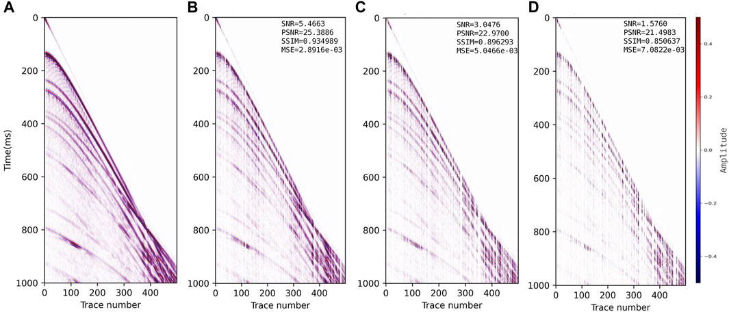
FIGURE 4. Experimental synthetic seismic data. (A) Complete seismic data. Spatially irregular data with sampling rates of (B) 70%, (C) 50% and (D) 30%.

FIGURE 5

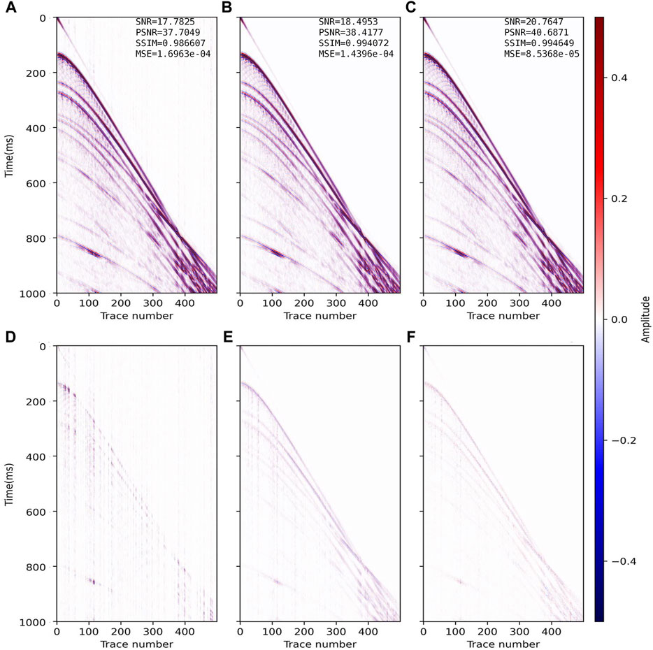
FIGURE 5. Reconstructed results and residual errors for the data (SR = 70%) in Figure 4C. The reconstruction results with (A) CS, (B) DnCNN and (C) CSDNN. (D–F) are the residual errors between the complete synthetic data in Figure 4A and panels (A–C) of this figure.

FIGURE 6

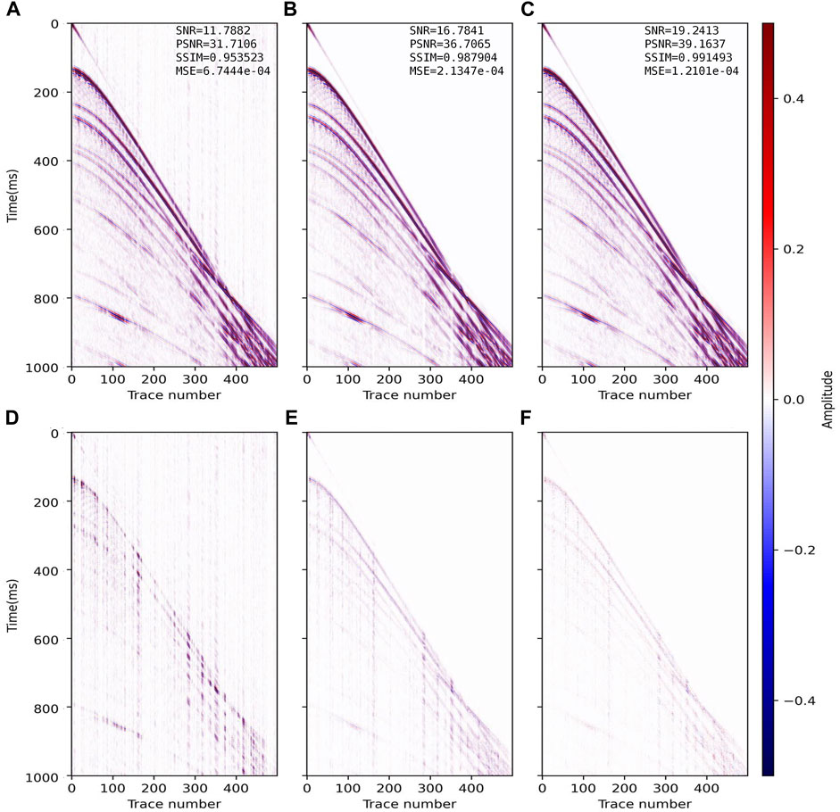
FIGURE 6. Reconstructed results and residual errors for the data (SR =50%) in Figure 4C. The reconstruction results with (A) CS, (B) DnCNN and (C) CSDNN. (D–F) are the residual errors between the complete synthetic data in Figure 4A and panels (A–C) of this figure.

FIGURE 7

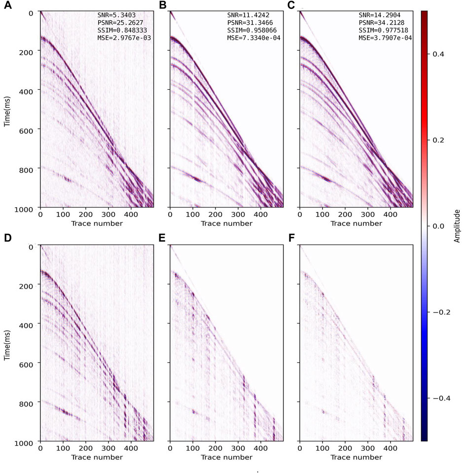
FIGURE 7. Reconstructed results and residual errors for the data (SR=30%) in Figure 4D. The reconstruction results with (A) CS, (B) DnCNN and (C) CSDNN. (D–F) are the residual errors between the complete synthetic data in Figure 4A and panels (A–C) of this figure.

FIGURE 8

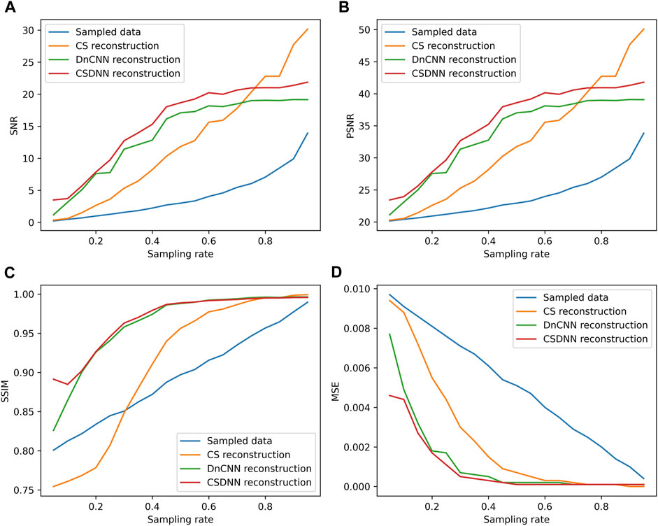
FIGURE 8. The curve of (A) SNR, (B) PSNR, (C) SSIM, and (D) MSE of the reconstruction effect.

From the reconstruction and residual profiles in Figures 5–7, the above three methods can effectively recover the information in few missing traces (SR=70%). As the SR gets lower, the CS-based reconstruction is the worst, and the SNR drops from 17.78 dB in Figure 5A to 5.34 dB in Figure 7A, which constitutes a decrease of 53%. It can be seen that the inadaptability of the CS method to low SR and spatially irregular data is obviously enhanced, which verifies the theoretical defect of the CS method in this case. The DnCNN-based reconstruction with SR = 50% (Figure 6B, SNR = 16.78 dB) is similar to the CS-based reconstruction with SR = 70% (Figure 5A, SNR = 17.78 dB), so the effect of DL method represented by DnCNN is better than CS. With more missing traces, the reconstruction SNR of the DnCNN drops from 18.50 dB in Figure 5B to 11.42 dB in Figure 7B, equivalent to a drop of 38%. This shows that when the difference between training data and labels is larger, the generalizability of the trained network model is weaker. Our CSDNN method indicates the best reconstruction performance at each SR, from 20.76 dB in Figure 5C to 14.29 dB in Figure 7C, equivalent to a decrease of 31%. Thus, CSDNN is more adaptable to the reconstruction of spatially irregular seismic data with low SR.

Figure 8 shows that when the SR is higher than 75%, the CS-based reconstruction has better SNR and PSNR than CSDNN. The reason is that the underdetermined degree of the objective function is low when the amount of data is large, which explains the rationality of obtaining credible CS reconstruction results for spatially irregular data under high SR even if it does not meet the requirements of CS theory. Another reason is that in the two methods related to learning, the SR used in the training data is 50%, which means that when the SR of the data to be reconstructed is very different from the training data, there will be a significant inadaptation, but the reconstruction of CSDNN is still better than DnCNN in this case. In other cases, CSDNN reconstruction has the highest SNR, PSNR, SSIM and the lowest MSE among the three methods. In fact, we usually focus on reconstruction with relatively low SR, so the result also verifies the effectiveness of reducing the difference between the training data and its labels for improving network generalizability.

3.2 Field data experiments

In order to further verify the generalizability of our method, the real marine seismic data (Figure 9A, with 430 traces, 512 samples in each trace, spatial interval is 12.5 m), is also randomly sampled in the spatial dimension with SR of 70% (Figure 9B), 50% (Figure 9C) and 30% (Figure 9D). Then, we reconstruct them using the above three methods, and the results and residuals are shown in Figures 10–12. The DnCNN and CSDNN methods here use the two network models trained in the above synthetic data experiment.

FIGURE 9

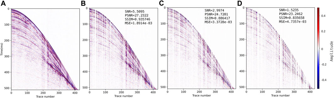
FIGURE 9. Field seismic data. (A) Complete field seismic data. Spatially irregular data with SR of (B) 70%, (C) 50% and (D) 30%.

FIGURE 10

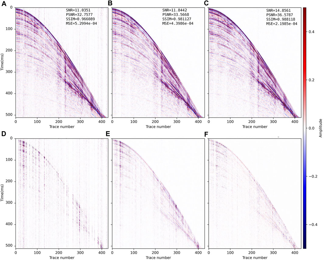
FIGURE 10. Reconstructed results and residual errors for the field data (SR =70%) in Figure 9B. The reconstruction results with (A) CS, (B) DnCNN and (C) CSDNN. (D–F) are the residual errors between the complete synthetic data in Figure 9A and panels (A–C) of this figure.

FIGURE 11

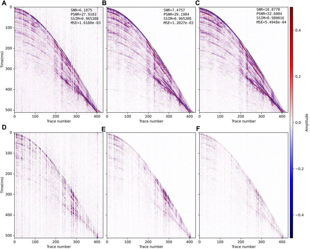
FIGURE 11. Reconstructed results and residual errors for the field data (SR=50%) in Figure 9C. The reconstruction results with (A) CS, (B) DnCNN and (C) CSDNN. (D–F) are the residual errors between the complete synthetic data in Figure 9A and panels (A–C) of this figure.

FIGURE 12

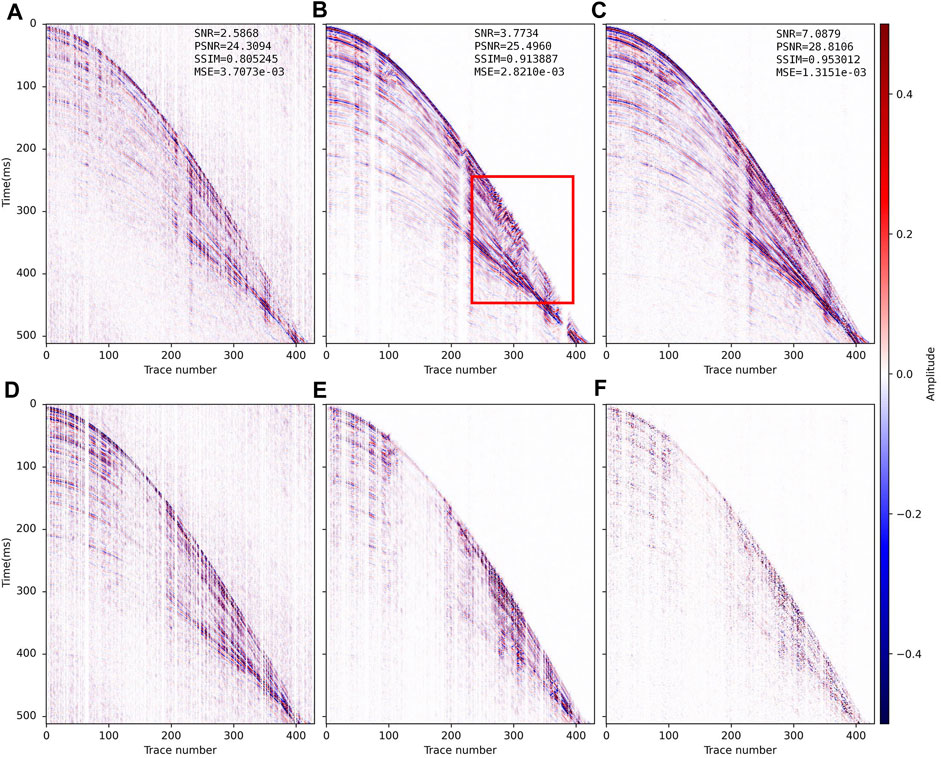
FIGURE 12. Reconstructed results and residual errors for the field data (SR = 30%) in Figure 9D. The reconstruction results with (A) CS, (B) DnCNN and (C) CSDNN. (D–F) are the residual errors between the complete synthetic data in Figure 9A and panels (A–C) of this figure.

When the field data misses few traces (SR = 70%), the CS reconstruction (Figure 10A, SNR=11.04 dB) is close to DnCNN (Figure 10B, SNR=11.84 dB). All three methods can reconstruct the field data well, but the CSDNN reconstruction result has the highest SNR (14.86 dB), PSNR (36.57 dB), SSIM (0.988), the lowest MSE (2.20e-04), and the strongest horizontal continuity, and can recover many small features. With lower SR, the CS reconstruction (Figure 11A, SNR = 6.18 dB; Figure 12A, SNR = 2.59 dB) shows event discontinuity and the noise is more obvious; the DnCNN reconstruction (Figure 11B, SNR = 7.48 dB; Figure 12B, SNR = 3.77 dB) is better than CS, but there is an apparent error in the reconstructed event at the continuous missing traces position (red mark in Figure 12B); CSDNN (Figure 11C, SNR=10.88 dB; Figure 12C, SNR=7.09 dB) combines the model-driven prior knowledge on the DnCNN, better guarantees the event continuity and correctness, and the reconstruction SNR is the highest. The inveracious reconstruction shown in Figure 12B does not meet the spatiotemporal variation rules of seismic data and also indicates the necessity of adding knowledge constraints to DL. The performance of our CSDNN method on the field data further proves its generalizability.

4 Discussions

Aimed at the reconstruction of spatially irregularly acquired seismic data, in this work, we considered it separately from the perspectives of the traditional and AI methods. On the one hand, we pointed out the theoretical flaw of CS reconstruction for such data and explained the reason why CS is difficult to obtain satisfactory reconstruction. On the other hand, we highlighted that the generalizability of DL under limited datasets is a crucial aspect that must be significantly enhanced before this method can be implemented in industrial applications. By summarizing the discussion about network complexity and generalization in statistical learning theory, and combining it with the nature of the seismic data reconstruction problem, our inference is that the approach for DL to train neural networks with excellent generalizability should be to minimize the difference between training data and labels.

Based on this reasoning, the proposed CSDNN method reduces this difference through the CS-based preliminary reconstruction, and takes DL to alleviate the reconstruction deficiency caused by the defect of applying CS theory, with the sparsity of the data as the domain knowledge. Tests conducted on both synthetic and field seismic data revealed that the CSDNN outperforms traditional CS and DNN methods. This superiority holds even at low sampling rates, affirming the viability, efficiency, and versatility of this approach.

Due to the fact that CSDNN method requires more processing to reconstruct based on CS than typical DL methods, one of its disadvantages are in terms of computational efficiency and amount. Another disadvantage is that we simply use the cascade connection to combine CS and DNN, and there is no further discussion of integrating domain knowledge into neural networks. We designed this form of tandem CS and DnCNN just to validate the inference that reducing the differences between labels and input data can improve the generalization ability. In fact, future research can be done on designing more flexible models that incorporate more domain knowledge and more fully and deeply into neural networks. Besides, the main limitation of this method is that supervised learning requires a large amount of completed data in network training, but it is difficult to obtain a large amount of field label data. Our next research will also focus on using unsupervised or weakly supervised methods to obtain better reconstruction results.

The strategy outlined in this paper is equivalent to feeding the network additional feature and constraint information during training, compacting the solution space to a more reasonable range and increasing the accuracy of data reconstruction at low sampling rates. Subsequent research endeavors will foster a closer integration between model-driven and data-driven methodologies.

5 Conclusion

According to the notion that imposing prior knowledge constraint in data-driven models may effectively improve the generalizability of DL, we proposed a CSDNN method combining the model-driven CS and the data-driven DnCNN method for spatially irregular seismic data reconstruction, and a step-by-step optimization algorithm was put forward by synthesizing their objective functions. The domain knowledge here is the sparsity of seismic data, which is governed by the wave equation and has a regular spatiotemporal variation. Based on this, a suitable sparse basis can be found for preliminary reconstruction with CS. Experiments proved that preliminary implementation of the data and model dual drive in the form of concatenation produced positive findings, which backed up our theory regarding the link between dataset differences and network generalizability. The direction of future research is to analyze the quantitative relationship among the complexity of the network model, the variation between training data and labels, and the network generalizability.

Data availability statement

The datasets presented in this article are not readily available because The data are not publicly available due to privacy restrictions. Requests to access the datasets should be directed to gongxinyue@zju.edu.cn.

Author contributions

XG: Conceptualization, Data curation, Formal Analysis, Investigation, Methodology, Software, Validation, Visualization, Writing–original draft, Writing–review and editing. SC: Conceptualization, Methodology, Supervision, Writing–review and editing. CJ: Data curation, Methodology, Writing–review and editing.

Funding

The author(s) declare financial support was received for the research, authorship, and/or publication of this article. This work was supported by the National Natural Science Foundation of China under Grant 42274145.

Conflict of interest

The authors declare that the research was conducted in the absence of any commercial or financial relationships that could be construed as a potential conflict of interest.

Publisher’s note

All claims expressed in this article are solely those of the authors and do not necessarily represent those of their affiliated organizations, or those of the publisher, the editors and the reviewers. Any product that may be evaluated in this article, or claim that may be made by its manufacturer, is not guaranteed or endorsed by the publisher.

Abbreviations

CS, Compressed sensing; DNN, Deep neural network; DL, Deep learning; DnCNN, Denoising convolutional neural network; CSDNN, Our method based on CS and DNN; SNR, Signal-to-noise ratio; PSNR, Peak signal-to-noise ratio; SSIM, Structural similarity index method; MSE, Mean square error; $\delta \left(f\right)$, Dirac delta function; IST, Iterative Soft Thresholding; DCT, Discrete cosine transform; SR, Sampling rate; $\mathit{W}$, Sampling matrix; $\mathit{d}$, Observed signal/data; $\mathit{u}$, Original signal/data; $M$, Number of regular sampling points; $N$, Number of irregular sampling points; $\mathbb{R}$, Field of real numbers; $\mathbf{c}$, Sparse transform coefficient; $\mathrm{\Phi }$, Sparse transformation; $\mathbf{S}$, Sensing matrix; $\lambda$Regularization parameter; ${\mathit{u}}_{lab}$, complete seismic data in training dataset; ${\mathit{d}}^{cs}$, CS-based reconstruction of $\mathit{d}$; $\widehat{\mathit{u}}$, Reconstruction data.

References

Abma, R., and Kabir, N. (2006). 3D interpolation of irregular data with a POCS algorithm. Geophysics 71, E91–E97. doi:10.1190/1.2356088

CrossRef Full Text | Google Scholar

Candès, E. J., Romberg, J., and Tao, T. (2006). Robust uncertainty principles: exact signal reconstruction from highly incomplete frequency information. IEEE Trans. Inf. Theory 52, 489–509. doi:10.1109/TIT.2005.862083

CrossRef Full Text | Google Scholar

Chai, X., Gu, H., Li, F., Duan, H., Hu, X., and Lin, K. (2020). Deep learning for irregularly and regularly missing data reconstruction. Sci. Rep. 10, 3302. doi:10.1038/s41598-020-59801-x

PubMed Abstract | CrossRef Full Text | Google Scholar

Chen, G.-X., Chen, S.-C., Wang, H.-C., and Zhang, B. (2013). Geophysical data sparse reconstruction based on L0-norm minimization. Appl. Geophys. 10, 181–190. doi:10.1007/s11770-013-0380-6

CrossRef Full Text | Google Scholar

Donoho, D. L. (2006a). Compressed sensing. IEEE Trans. Inf. Theory 52, 1289–1306. doi:10.1109/TIT.2006.871582

CrossRef Full Text | Google Scholar

Donoho, D. L. (2006b). Compressed sensing. IEEE Trans. Inf. Theory 52, 1289–1306. doi:10.1109/TIT.2006.871582

CrossRef Full Text | Google Scholar

Dou, Y., Li, K., Duan, H., Li, T., Dong, L., and Huang, Z. (2023). MDA GAN: adversarial-learning-based 3-D seismic data interpolation and reconstruction for complex missing. IEEE Trans. Geosci. Remote Sens. 61, 1–14. doi:10.1109/TGRS.2023.3249476

CrossRef Full Text | Google Scholar

Fang, W., Fu, L., Liu, S., and Li, H. (2021a). Dealiased seismic data interpolation using a deep-learning-based prediction-error filter. GEOPHYSICS 86, V317–V328. doi:10.1190/geo2020-0487.1

CrossRef Full Text | Google Scholar

Fang, W., Fu, L., Zhang, M., and Li, Z. (2021b). Seismic data interpolation based on U-net with texture loss. Geophysics 86, V41–V54. doi:10.1190/geo2019-0615.1

CrossRef Full Text | Google Scholar

Hennenfent, G., Fenelon, L., and Herrmann, F. J. (2010). Nonequispaced curvelet transform for seismic data reconstruction: a sparsity-promoting approach. GEOPHYSICS 75, WB203–WB210. doi:10.1190/1.3494032

CrossRef Full Text | Google Scholar

Herrmann, F. J., and Hennenfent, G. (2008). Non-parametric seismic data recovery with curvelet frames. Geophys. J. Int. 173, 233–248. doi:10.1111/j.1365-246X.2007.03698.x

CrossRef Full Text | Google Scholar

Ibrahim, A., Terenghi, P., and Sacchi, M. D. (2018). Simultaneous reconstruction of seismic reflections and diffractions using a global hyperbolic Radon dictionary. GEOPHYSICS 83, V315–V323. doi:10.1190/geo2017-0655.1

CrossRef Full Text | Google Scholar

Innocent Oboué, Y. A. S., Chen, W., Wang, H., and Chen, Y. (2021). Robust damped rank-reduction method for simultaneous denoising and reconstruction of 5D seismic data. Geophysics 86, V71–V89. doi:10.1190/geo2020-0032.1

CrossRef Full Text | Google Scholar

Liu, D., Wang, W., Wang, X., Wang, C., Pei, J., and Chen, W. (2020). Poststack seismic data denoising based on 3-D convolutional neural network. IEEE Trans. Geosci. Remote Sens. 58, 1598–1629. doi:10.1109/TGRS.2019.2947149

CrossRef Full Text | Google Scholar

Luo, C., Ba, J., and Guo, Q. (2023). Probabilistic seismic petrophysical inversion with statistical double-porosity Biot-Rayleigh model. GEOPHYSICS 88, M157–M171. doi:10.1190/geo2022-0288.1

CrossRef Full Text | Google Scholar

Mousavi, S. M., and Beroza, G. C. (2022). Deep-learning seismology. Science 377, eabm4470. doi:10.1126/science.abm4470

PubMed Abstract | CrossRef Full Text | Google Scholar

Mousavi, S. M., Langston, C. A., and Horton, S. P. (2016). Automatic microseismic denoising and onset detection using the synchrosqueezed continuous wavelet transform. Geophysics 81, V341–V355. doi:10.1190/geo2015-0598.1

CrossRef Full Text | Google Scholar

Naghizadeh, M., and Innanen, K. A. (2011). Seismic data interpolation using a fast generalized Fourier transform. GEOPHYSICS 76, V1–V10. doi:10.1190/1.3511525

CrossRef Full Text | Google Scholar

Oropeza, V., and Sacchi, M. (2011). Simultaneous seismic data denoising and reconstruction via multichannel singular spectrum analysis. Geophysics 76, V25–V32. doi:10.1190/1.3552706

CrossRef Full Text | Google Scholar

Pan, X., Wu, H., Chen, Y., Qin, Z., and Wen, X. (2023). The interplay of framelet transform and l_p quasi-norm to interpolate seismic data. IEEE Geosci. Remote Sens. Lett. 20, 1–5. doi:10.1109/LGRS.2022.3227567

CrossRef Full Text | Google Scholar

Pham, N., and Li, W. (2022). Physics-constrained deep learning for ground roll attenuation. GEOPHYSICS 87, V15–V27. V15–V27. doi:10.1190/geo2020-0691.1

CrossRef Full Text | Google Scholar

Piela, L. (2014). “Dirac delta function,” in Ideas of quantum chemistry (Elsevier), e69–e72. doi:10.1016/B978-0-444-59436-5.00025-8

CrossRef Full Text | Google Scholar

Ronen, J. (1987). Wave-equation trace interpolation. GEOPHYSICS 52, 973–984. doi:10.1190/1.1442366

CrossRef Full Text | Google Scholar

Sang, W., Yuan, S., Han, H., Liu, H., and Yu, Y. (2023). Porosity prediction using semi-supervised learning with biased well log data for improving estimation accuracy and reducing prediction uncertainty. Geophys. J. Int. 232, 940–957. doi:10.1093/gji/ggac371

CrossRef Full Text | Google Scholar

Song, C., and Wang, Y. (2023). Simulating seismic multifrequency wavefields with the Fourier feature physics-informed neural network. Geophys. J. Int. 232, 1503–1514. doi:10.1093/gji/ggac399

CrossRef Full Text | Google Scholar

Spitz, S. (1991). Seismic trace interpolation in the F-X domain. GEOPHYSICS 56, 785–794. doi:10.1190/1.1443096

CrossRef Full Text | Google Scholar

Sun, J., Niu, Z., Innanen, K. A., Li, J., and Trad, D. O. (2020). A theory-guided deep-learning formulation and optimization of seismic waveform inversion. GEOPHYSICS 85, R87–R99. doi:10.1190/geo2019-0138.1

CrossRef Full Text | Google Scholar

Sun, Y.-Y., Jia, R.-S., Sun, H.-M., Zhang, X.-L., Peng, Y.-J., and Lu, X.-M. (2018). Reconstruction of seismic data with missing traces based on optimized Poisson Disk sampling and compressed sensing. Comput. Geosci. 117, 32–40. doi:10.1016/j.cageo.2018.05.005

CrossRef Full Text | Google Scholar

Trad, D. (2003). Interpolation and multiple attenuation with migration operators. GEOPHYSICS 68, 2043–2054. doi:10.1190/1.1635058

CrossRef Full Text | Google Scholar

Vapnik, V. N. (1999). An overview of statistical learning theory. IEEE Trans. Neural Netw. 10, 988–999. doi:10.1109/72.788640

PubMed Abstract | CrossRef Full Text | Google Scholar

Wang, B., Wu, R.-S., Chen, X., and Li, J. (2015). Simultaneous seismic data interpolation and denoising with a new adaptive method based on dreamlet transform. Geophys. J. Int. 201, 1182–1194. doi:10.1093/gji/ggv072

CrossRef Full Text | Google Scholar

Wang, B., Zhang, N., Lu, W., and Wang, J. (2019). Deep-learning-based seismic data interpolation: a preliminary result. GEOPHYSICS 84, V11–V20. doi:10.1190/geo2017-0495.1

CrossRef Full Text | Google Scholar

Wang, Y., Zhou, H., Zu, S., Mao, W., and Chen, Y. (2017). Three-operator proximal splitting scheme for 3-D seismic data reconstruction. IEEE Geosci. Remote Sens. Lett. 14, 1830–1834. doi:10.1109/LGRS.2017.2737786

CrossRef Full Text | Google Scholar

Wu, X., Ma, J., Si, X., Bi, Z., Yang, J., Gao, H., et al. (2023). Sensing prior constraints in deep neural networks for solving exploration geophysical problems. Proc. Natl. Acad. Sci. 120, e2219573120. doi:10.1073/pnas.2219573120

PubMed Abstract | CrossRef Full Text | Google Scholar

Wu, X., and Zhang, J. (2017). Researches on rademacher complexities in statistical learning theory: a survey. Acta Autom. Sin. 43, 20–39. doi:10.16383/j.aas.2017.c160149

CrossRef Full Text | Google Scholar

Yin, X.-Y., Liu, X.-J., and Zong, Z.-Y. (2015). Pre-stack basis pursuit seismic inversion for brittleness of shale. Pet. Sci. 12, 618–627. doi:10.1007/s12182-015-0056-3

CrossRef Full Text | Google Scholar

Yuan, S., Jiao, X., Luo, Y., Sang, W., and Wang, S. (2022). Double-scale supervised inversion with a data-driven forward model for low-frequency impedance recovery. GEOPHYSICS 87, R165–R181. doi:10.1190/geo2020-0421.1

CrossRef Full Text | Google Scholar

Zhao, Y., Niu, F.-L., Fu, L., Cheng, C., Chen, J.-H., and Huo, S.-D. (2021). Local events-based fast RTM surface-offset gathers via dip-guided interpolation. Pet. Sci. doi:10.1007/s12182-021-00557-y

CrossRef Full Text | Google Scholar

Zhong, W., Chen, Y., and Gan, S. (2015). Irregularly sampled 3D seismic data reconstruction with L1/2 norm regularization. Madrid, Spain. doi:10.3997/2214-4609.201413447

CrossRef Full Text | Google Scholar

Zwartjes, P., and Gisolf, A. (2006). Fourier reconstruction of marine-streamer data in four spatial coordinates. GEOPHYSICS 71, V171–V186. doi:10.1190/1.2348633

CrossRef Full Text | Google Scholar