 Youtao Wang
 Xiong Ma1,2*
95% of researchers rate our articles as excellent or good
Learn more about the work of our research integrity team to safeguard the quality of each article we publish.
Find out more
ORIGINAL RESEARCH article
Front. Earth Sci. , 16 January 2024
Sec. Solid Earth Geophysics
Volume 11 - 2023 | https://doi.org/10.3389/feart.2023.1297501
This article is part of the Research Topic Advances of New Technologies in Seismic Exploration View all 22 articles
Seismic facies analysis is important for oil and gas exploration. The conventional seismic facies recognition methods are implemented manually with high workload and low accuracy. Therefore, how to obtain seismic facies characteristics quickly, efficiently, and accurately is an urgent requirement in seismic facies research. To alleviate this issue, we propose a novel seismic facies recognition method based on the region growing algorithm with expert knowledge constraint. The processes of this algorithm are as follows: firstly, we select high-density 3D seismic data in the target area for seismic facies identification. Then, we utilize expert knowledge to define the priori geological constraint for regional growing algorithm. Finally, the region growing algorithm is used to pick up and divide different 3D seismic facies boundaries in the study area. The verification of known geological knowledge proves that the results are reasonable and reliable. The accuracy and efficiency of the proposed seismic facies identification method based on region growing are significantly improved.
Sedimentary facies analysis is a fundamental work in hydrocarbon exploration, and its reliability directly determines the success or failure of petroleum exploration (Wang et al., 2002; Bao et al., 2005; Yang et al., 2010; Wu et al., 2011). Seismic facies can be explained as the sum of sedimentary facies expressed in seismic information, that is, seismic facies are seismic features formed by the sedimentary environment (Sloss, 1962; Xu et al., 1990). Therefore, the spatial distribution characteristics of sedimentary facies can be established by seismic facies analysis, combined with drilling, provenance direction, and other information (Zhang et al., 2001; Zhu et al., 2009).
With the widespread use of three-dimensional (3D) seismic data, the overall understanding of regional sedimentary facies is no longer limited to well data alone but is more often obtained through the analysis and conversion of seismic facies based on the calibration of well data. Thus, it is necessary for geologists to acquire seismic facies features faster and with higher accuracy. Several scholars have tried to explore seismic facies through seismic attributes (Zhang et al., 2010; Tang et al., 2011), waveform clustering (Deng et al., 2008; Li et al., 2017; Liu et al., 2020), shallow neural network similarity (Saggaf et al., 2003; Marroquín et al., 2009; Dramsch and Lüthje, 2018), deep learning (Wrona et al., 2018; Duan et al., 2019; Yan et al., 2020; He et al., 2022; Sang et al., 2023), and many other methods, and have achieved certain results. For example, He et al. (2022) used semi-supervised learning for intelligent seismic facies identification and obtained good results with improved estimation accuracy. Sang et al. used semi-supervised learning for porosity prediction and reduced the prediction uncertainty compared to conventional methods. The methods based on deep learning may encounter a common challenge, that is, deep networks trained for one region may be difficult to apply to other regions.
With the increasing precision and depth of exploration, the correlation between sedimentary facies models and geophysical data such as seismic and well logging becomes more and more complicated. It is difficult to identify the above complex relationships by only interpreting sedimentary facies patterns manually, and the accuracy and efficiency of manual interpretation cannot meet the current needs of efficient exploration in the oilfield. Therefore, it is necessary to introduce new seismic facies identification techniques to realize efficient and accurate recognition of 3D seismic facies.
Image segmentation is one of the fundamental and key aspects in the field of computer vision. Region growing is proposed under this background and has been widely used in the field of automatic image segmentation. Its biggest advantage is the integration of a priori expert knowledge, which is suitable for the recognition and division of equally complex seismic images (Zhu et al., 1996; Zhou et al., 2017). Herein, based on the region growing algorithm, we can obtain the sensitive attributes of seismic facies through optimization, and define the seed points, growth criteria, and growth cut-off conditions for regional growth based on a priori geological understanding of the isochronous slice of the Wheeler domain. Then, we can recognize the seismic facies layer by layer, and synthesize the final 3D seismic facies identification results by interpolation in 3D space, which greatly improves the accuracy and efficiency of seismic facies recognition.
Region growing is a method of aggregating pixel points according to the similarity of pixels within the same zone. Starting from an initial area, such as a single pixel, the region is gradually grown by subsuming adjacent pixels with the same properties until there are no more points to be grouped (Meyer, 1990; Adams et al., 1994; Mehnert and Jackway, 1997). Herein, the general process of implementing the region growing algorithm can be carried out according to the following steps:
(1) In one image, non-edge or smooth points are manually or automatically selected as seed points, and each seed region is labeled using an agreed different value. Meanwhile, the mean value of each seed area is calculated, and then the value of the pixel points is replaced with the mean value.
(2) the non-edge and unmarked pixel point is located, marked as Point Q, and the distance between the Point Q and the region where the eight-neighbor pixel is situated further calculated, which means the minimum distance can be obtained. The distance mentioned above is given by Eq. 1:
where (L*, a*, b*) denotes the values of unlabeled pixel points on the three components of L*, a*, b*, respectively, and
The calculation allows Point Q to be assigned to the region where the minimum distance neighborhood point is located, and then further update the mean value of the region and the value of the pixel. The above steps should be repeated until all pixel points excluding edge points are marked.
(3) In order to maintain the distinct edges between large regions, it is necessary to mark the edge points after non-edge points. Specifically, this means finding the pixel points of edge point mapping EM (i, j) = 1 in the complex wavelet domain, and contining to repeat step (2) until all edge pixel points are labeled.
(4) In order to solve the over-segmentation problem caused by too many seed points and to obtain better results for human senses, it is necessary to perform region merging based on the following two merging criteria:
a. The distance among adjacent regions is taken as the base, and the Euclidean distance between the mean value of the region to be merged and the adjacent region is calculated by Eq. 2:
where
If the d is less than the threshold δ, the two regions are combined and the mean value of the regions is recalculated.
b. If the ratio of the region size to the image size is less than the preset ratio threshold μ, the calculated region is merged with the neighboring region with the smallest surrounding color distance.
(5) Through the optimization of similar regions by multiple iterations, we achieve the image segmentation.
In seismic interpretation, seismic facies recognition is usually done by initially filtering out sensitive seismic attribute slices and then manually mapping different seismic facies on seismic attribute slices. This traditional method is very laborious, and it is easy to ignore the characteristics of the image itself and add too much subjective judgment. The region growing algorithm can fully utilize the searching and processing capability of the computer to extract more potential information in the image and achieve fast and accurate segmentation of seismic facies image, thereby greatly improving the accuracy and efficiency of seismic facies analysis.
However, the seismic facies images have multiple interpretations compared to conventional images. For example, two regions with the same color but not connected may belong to different types of sedimentary facies, or regions with different colors may belong to the same types of sedimentary facies. Therefore, when using the region growing algorithm to segment seismic facies images, there is a high possibility of over-segmentation or under-segmentation, which will reduce the geological significance of the results.
In this paper, we select high-density 3D seismic data in the Moxizhuang area in the Junggar Basin for 3D seismic facies identification with the regional growing algorithm. Based on expert knowledge to define initial seed points, regional growing criteria, and vertical cut-off condition as a priori geological constraint, the region growing algorithm is used to pick up and divide different 3D seismic facies boundaries in the study area to solve over-segmentation or under-segmentation problems in seismic facies analysis.
To obtain the results of 3D seismic facies identification in the study area, we firstly carried out the seismic phase boundary classification and identification by using a computer to slice layer by layer at a vertical resolution. Figure 1 shows the N-S-direction seismic profile and horizontal time slice in the study area. In this profile, the diachroneity is very obvious on the contemporaneous horizontal slice. The seismic facies has rapidly variable lateral phase changes and cannot establish an accurate relationship with the actual sedimentary interface. Therefore, it is difficult to identify seismic facies boundaries from isochronous slices of original seismic data using the region growing algorithm, and the accuracy is relatively low.
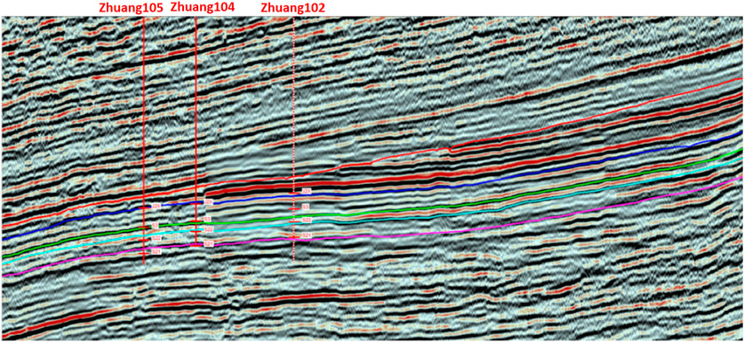
FIGURE 1. Near N-S-direction seismic profile in the time domain through wells Zhuang105-Zhuang104-Zhuang102.
To better solve the diachronous problem, we transformed the seismic data volume or sensitive attribute volume in the time domain to that in the Wheeler domain (relative geologic age domain), and then identified the seismic facies boundary on the slices of the Wheeler domain. On the basis of detailed identification of seismic isochronous interface, we built a sedimentary model that is more consistent with the actual geological conditions, and developed Wheeler domain transformation that is more consistent with the actual geological significance (Tan, 2013; Forte et al., 2016; Yin et al., 2018). Under certain resolution conditions, the transformed seismic syncphase axis is nearly horizontal and has better isochronism. The stratigraphic cyclicity is clearer, which can better reveal the spatial relationship among sedimentary elements (Figure 2).
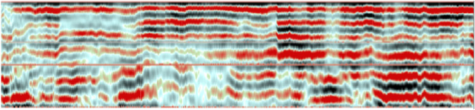
FIGURE 2. Local scale of the near N-S-direction seismic profile in the Wheeler domain through wells Zhuang105-Zhuang104-Zhuang102, Lower Jurassic Sangonghe Formation.
Next, the extraction of densely sampled isochronous slices is achieved by extracting slices from the sampled points of the Wheeler domain seismic data volume or sensitive attribute data volume of the vertical seismic profile. The geological significance of each slice is relatively clear, with better correspondence with sedimentary facies. This facilitates the identification of seismic facies boundary by using region growing, and then transforms to sedimentary facies boundary to achieve geologically meaningful 3D seismic facies recognition.
Since the multi-solution of seismic interpretation leads to more complex segmentation and recognition of seismic phase images, a recognition algorithm with human-computer interaction for improving accuracy is needed. The region growing algorithm selects pixels with similar features and merges them into regions. There are three major factors affecting the algorithm: the initial seed points, the region growing criteria, and the vertical cutoff conditions. The optimal determination of these three elements using expert knowledge can better introduce the a priori geological knowledge into the seismic facies identification.
The initial seed point is the pixel that can represent most of the pixels in the target region, and its accuracy has a great influence on the recognition result of the region growing algorithm. Generally, there are two methods of seed point selection: (1) automatic selection of the seed point based on non-edge and smooth points, and (2) Manual selection of the seed point based on expert knowledge. The former can save a lot of manpower and time by automatically selecting the seed point through considering edge and pixel information of color images. However, there are also a series of problems such as over-selection and atypical selection, especially when facing complex images such as a seismic facies diagram. It is not only difficult to select appropriate initial seed points, but also to introduce the existing geological understanding into the segmentation calculation. Therefore, in this paper, the initial seed points are manually selected based on expert knowledge. Although the cost of labor and time is slightly increased, this method can better offset the false segmentation of seismic phase generated by seismic multi-solution and is more consistent with geological understanding.
In this paper, the manual selection of the initial seed points is mainly based on the following two principles:
(1) The well point on each slice must be selected as the initial seed point. Geologists interpret well logging facies according to logging, coring, and other existing geological data to ensure maximum reliability of the geological results. With the detailed well-seismic calibration, the logging phase of a single well can be precisely corresponded to the seismic traces beside the well. On this basis, the well logging facies can assign sedimentary facies’ geological significance to the 3D seismic facies picked up near the well, thus achieving the hard constraints on the geological conclusions of the well logging during the regional growth.
(2) Non-well points screened by geologists that can reflect the typical morphology of the sedimentary facies can also be used as initial seed points. Based on the correspondence between existing sedimentary models and seismic attributes, and combined with the understanding of existing sedimentary characteristics, geologists can identify the typical attribute distribution characteristics of different sedimentary facies in sensitive attribute slices. This kind of non-well point can be used as initial seed points for non-well stations, thus making up for the fact that some logging facies types at well sites are scarce.
In the actual calculation process, we set different influence weights for manually selecting initial seed points. For example, the target layer in the region is mainly shallow delta front subfacies, and the weight of seed points involving shallow delta front subfacies in this layer segment will be set higher than that of coastal shallow lake subfacies. The specific weight ratio is given based on existing geological knowledge. This is also a control strategy based on expert knowledge (prior geological understanding).
Another key point in the region growing process is the selection of appropriate growth criteria. Region growing criteria can be developed based on different principles, and different growth criteria can result in different regional growth process. It has two major methods for setting region growing criteria, that is, the range of seismic attribute values and the correlation with seed points.
(1) Region growing criteria using the range of seismic attribute value. The geologists should prefer seismic attributes that can better reflect the sedimentary facies. After obtaining a range of seismic attribute values corresponding to different sediments using geophysical analysis, we then adjust the range of different attribute values to control the region growing of different seismic facies boundaries. This method has low requirements on initial seed points and is suitable for picking up multiple seismic facies boundaries simultaneously by using attribute value range constraints. However, it requires multiple seismic phases in the plane corresponding to the same sedimentary facies type.
(2) The region growing criteria by correlation with the seed point. The geologists also need to first select the seismic attribute that can better reflect the sedimentary facies, and then determine the initial seed points and calculate the average of the attributes for one or more seed points. The region growing condition is based on the correlation between the surrounding attribute values and the average of the seed point attributes, which has the minimum growth value corresponding to the lower limit of the correlation. This method relies on the selection of initial seed points by the geologist and enables controlled pickup of a single specific seismic phase boundary.
We identified and compared the seismic facies using the above two methods for amplitude attribute slices in the relative chronostratigraphic domain (Figure 3A). The results show that the seismic phase ranges identified using the attribute value range method are coarser, and it is easier to identify the non-seed point identification regions, which results in the under-segmentation of the seismic phases (Figure 3B). In contrast, the seismic phase range identified by the correlation with seed points method are narrower and the results had better correlation with the seed points (Figure 3C).
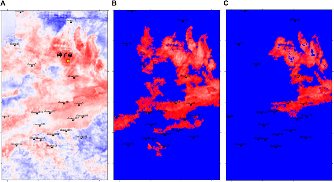
FIGURE 3. Comparison of the boundary range of seismic phase identified by two methods. (A) amplitude attribute slice in the relative chronostratigraphic domain; (B) attribute value method with picking up boundary range from15000 to 18,000; (C) correlation method with seed points with correlation coefficient 0.8.
Considering the advantages and limitations of the above two methods, the correlation with seed points is more suitable as a criterion for region growing. This is because the latter method provides more accurate identification and classification of seismic facies by manually preferring the initial seed points of different geological significance.
After determining the regional growth criteria, strata slices can be selected layer by layer for seismic facies identification and division. However, the cut-off conditions for the growing region in the vertical direction is still unclear. The initial seed point has a good representation of the seismic facies around it in one strata slice which can be approximated as an isochronous plane. Thus, it is reasonable to take the lower value of the correlation degree with the initial seed point as the cut-off condition for region growing. When another strata slice is vertically transformed, the corresponding sedimentary microfacies on the well may have changed significantly, although the change in properties may be minor. In this case, the correlation with the initial seed point can no longer fully express the change of geological significance of seismic facies, so it is necessary to further add an external hard constraint condition to correct this error.
The above problem can be solved by introducing the sedimentary facies information of a single well. The precise correspondence between the sedimentary microfacies on the well and the seismic traces beside the well can be established by using the fine well seismic calibration. Furthermore, the depth range of different sedimentary facies at the well point can be taken as the cut-off conditions for vertical growth of different seismic facies. Figure 4 shows the synthetic seismic records and logging facies of the Well Zhuang 3 in the study area. We took the underwater distributary channel at 3132 ms–3140 ms as an example. In the strata slices in the vertical range from 3132 ms to 3140 ms, the attribute scope near the initial seed point of the Well Zhuang 3 with its correlation degree greater than 0.8 can be identified as the underwater distributary channel. Meanwhile, the attribute scope near the initial seed point of the Well Zhuang 3 with its correlation degree greater than 0.8 in the strata slices from 3140 ms to 3146 ms should be described as channel bar microfacies.
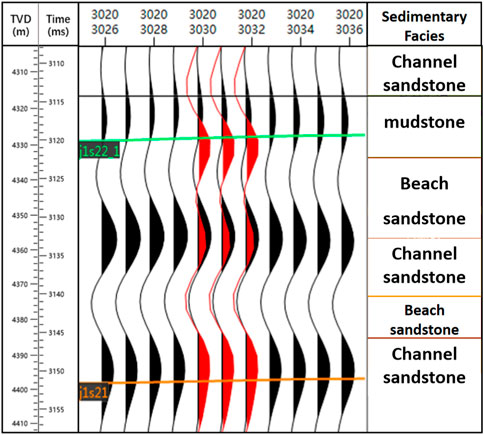
FIGURE 4. Fine calibration between the in-well sedimentary facies of the Well Zhuang 3 and well-side seismic trace.
In order to further break through the 2D seismic facies analysis and realize the 3D seismic facies modeling, we can extract dense strata slices at the interval of seismic vertical sampling rates from the seismic attribute data volume in the relative geological age domain (Wheeler domain). Then, we can identify and divide the seismic facies of the strata slices based on the regional growth algorithm and combine and smooth the recognition results of each slice within the three-dimensional space, so as to obtain the 3D seismic facies identification results.
In the previous exploration, a total of 20 exploratory wells were completed in the Jurassic strata in the Moxizhuang area and hinterland of the Junggar Basin, of which 5 wells were drilled and encountered oil flow, showing a great exploration potential. However, there were also some problems, such as the large buried depth of the target formation, poor correspondence between the reservoir and the seismic, and difficulty in accurately determining the distribution characteristics of sedimentary facies. In this study, the initial seed point, regional growth criteria, and vertical cut-off conditions were determined through expert knowledge to introduce geological constraints. On this basis, different 3D seismic facies boundaries were picked and divided by the regional growth algorithm to construct the 3D seismic facies model of the study area. Based on the interpretation of logging facies from real drilling, we have carried out a detailed description of sedimentary development characteristics in the study area.
The Jurassic Member 2 of Sangonghe Formation (J1s2) in the study area is vertically divided into five sandbed groups (from 1 to 5), among which 1, 2, 3, and 4 sandbodies are developed. From the thickness statistics of the J1s2 and the sandbodies from1 to 4, the shallow water delta frontal subfacies sedimentary system from the northern provenance is mainly developed in the study area during this period. Typical shallow water deltaic markers such as large amounts of carbon debris and vertical biological boreholes are also visible in the rock cores. The paleolandscape slope is gentle, at only about 0.3˚-1.4˚. The water depth is shallow, about 10–30 m, but with the deepening of the water body, the sandbodies presented the characteristics of multi-stage development and positive superposition. Through the optimization of seismic attributes by geologists, the root mean square amplitude is taken as the sensitive data body for seismic facies analysis, and isochronous strata slices are extracted at intervals of vertical seismic sampling rate for the root mean square amplitude attribute body in the Wheeler domain. Then, the regional growth algorithm can carry out the identification and division of different seismic facies in each strata slice. Finally, the results of seismic facies division in all strata slices are synthesized into 3D seismic facies recognition results in space. The whole process took about 5 h.
Figure 5 shows the near north-south seismic connecting-well profile of the Zhuang 103-Zhuang 2-Zhuang 1-Zhuang 104-Zhuang 101-Zhuang 107-Zhuang 3-Zhuang 301 wells extracted from the 3D seismic facies identification results. The sand content of the J1S2 2 formation is relatively low and the lithology is mainly sand-mud interbedded, in which the sand body is thin and laterally discontinuous, showing a shore shallow lake and delta front sedimentary facies. The sand content of the J1S1 2 formation is relatively high, with large sand body thickness and good lateral continuity, mainly manifesting as a shallow water delta front subfacies. The river channel migrated rapidly laterally, and the sedimentary microfacies dominated by the river channel sand bar changed rapidly longitudinally and laterally. The macroscopic sedimentary pattern shown in the seismic connecting-well profile is basically consistent with the existing geological understanding, and the description of different seismic facies is more refined. Figure 6 shows Logging facies profile of the connecting-well profile. Through comparison with the sedimentary facies profiles of the over-connected well, it is considered that the seismic facies identification results show more natural distribution characteristics of different facies zones with a certain vertical resolution and have good comparability with the actual sedimentary development characteristics.
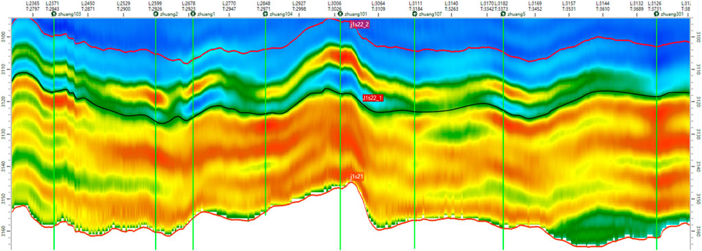
FIGURE 5. Seismic connecting-well profile of the Zhuang 103-Zhuang 2-Zhuang 1-Zhuang 104-Zhuang 101-Zhuang 107-Zhuang 3-Zhuang 301 wells.
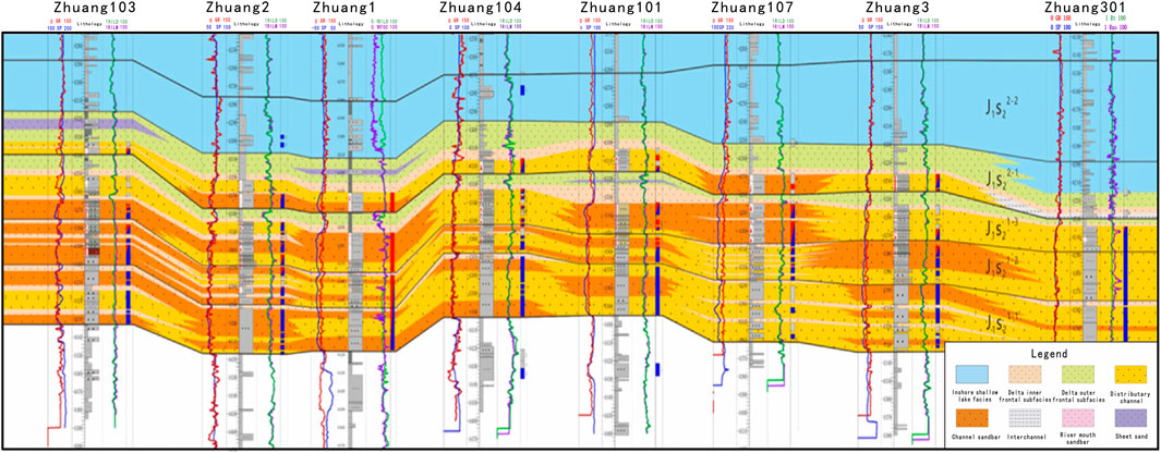
FIGURE 6. Logging facies profile of the Zhuang 103-Zhuang 2-Zhuang 1-Zhuang 104-Zhuang 101-Zhuang 107-Zhuang 3-Zhuang 301 wells.
The seismic facies map extracted from Sandbed Group 1 and Sandbed Group2 of the J1s1 2 strata are compared with the sedimentary facies diagram drawn by the geologists through the combination of well data and seismic data (Figures 7, 8). The results show that the automatic identification of seismic facies based on region growing was basically consistent with the distribution characteristics of different seismic facies in the original seismic data. The results also show that the automatic identification of seismic phases based on region growing is consistent with the spreading characteristics of different phases in the original seismic data. The results also show that it has a better effect on the mapping of different subfacies at the front edge of the shallow water delta in the study area, and the lateral distribution characteristics of different sedimentary facies zones are more refined and consistent with the geological deposition pattern. The seismic facies predicted by the proposed method are controlled by the category of seed points. For example, the seed points have been assigned five microfacies that belong to two different sedimentary subfacies. The predicted microfacies will not exceed the number of types given by the seed points. In summary, this has a good guiding significance for the understanding of sedimentary facies in the area.
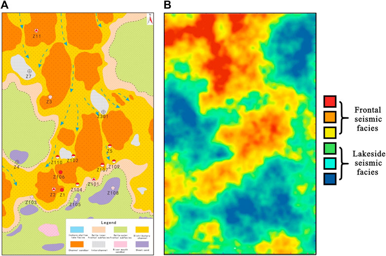
FIGURE 7. Sedimentary facies versus seismic facies for Sandbed Group 1 of the J1s1 2 strata. (A) Sedimentary facies diagram of Sandbed Group 1 of the J1s1 2 strata; (B) Seismic facies diagram of Sandbed Group 1 of the J1s1 2 strata.
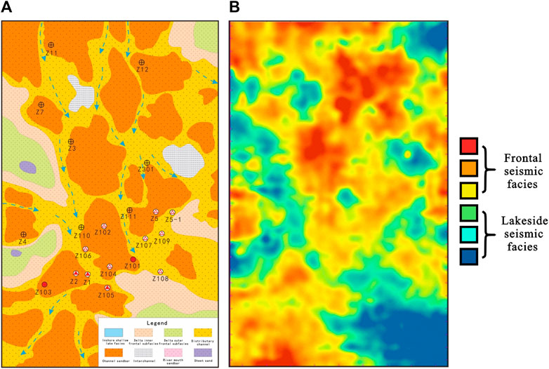
FIGURE 8. Sedimentary facies versus seismic facies for Sandbed Group 2 of the J1s1 2 strata. (A) Sedimentary facies diagram of Sandbed Group 2 of the J1s1 2 strata; (B) Seismic facies diagram of Sandbed Group 2 of the J1s1 2 strata.
Figure 9 shows the 3D display of seismic facies identification results from the bottom of J1S2 2 formation to the bottom of J1S1 2 formation in the study area relative to the chronostratigraphic domain restored to the temporal domain. Combined with the logging facies interpreted by real drilling, it can be found that the bottom of J1S2 2 formation is dominated by cold-toned shore-shallow lake seismic facies, but the local area also developed warm-toned front seismic facies from the northern provenance. The J1S2 2 formation generally showed a water-continent connection facies, and its lithology was dominated by sandstone-mudstone interbed. The J1S1 2 formation has an overall development of warm-toned frontal seismic facies, and its lithology was mainly sandstone, which is basically consistent with the actual geological understanding.
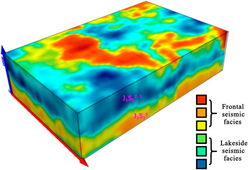
FIGURE 9. Seismic facies identification results of Jurassic Sangonghe Formation (time domain).
(1) The region growth algorithm based on the facet model can fully utilize the powerful processing ability of the computer to extract more potential information from sensitive attribute slices, effectively avoid over-segmentation, and realize the rapid and accurate segmentation of seismic facies images, which greatly improves the accuracy and efficiency of seismic facies analysis.
(2) Considering the three key elements of region growing, namely, initial seed point, regional growth criteria, and vertical cut-off conditions, a specific implementation strategy based on expert knowledge is innovatively proposed to introduce the priori geological knowledge into the specific seismic facies identification calculation through human-computer interaction, and more accurate seismic facies segmentation results can be obtained.
(3) This method has achieved good application results in the Moxizhuang area. The 3D seismic facies pickup results showed that the Jurassic Sangonghe Formation as a whole is dominated by northern provenance, and the bottom of J1S2 2 formation is dominated by shore-shallow lake facies. The front subfacies are developed in the local area, which is generally characterized by a water-continent connection facies with low sandstone ratio, and the lithology is dominated by sandstone-mudstone interbed, while the J1S1 2 formation is dominated by a shallow water delta front subfacies, and the river quickly migrated laterally with a high sandstone ratio, and the lithology is mainly sandstone (Su-Mei et al., 2022).
The raw data supporting the conclusion of this article will be made available by the authors, without undue reservation.
YoW: Conceptualization, Investigation, Methodology, Writing–original draft. XM: Data curation, Formal Analysis, Funding acquisition, Resources, Supervision, Validation, Writing–review and editing. ZG: Funding acquisition, Supervision, Validation, Writing–review and editing, Project administration. XC: Writing–review and editing, Resources, Validation. YuW: Writing–review and editing, Project administration.
The author(s) declare financial support was received for the research, authorship, and/or publication of this article. This research was financially funded by the China Postdoctoral Science Foundation (Certificate Number: 2023M730364) and Key Laboratory of Exploration Technologies for Oil and Gas Resources (Yangtze University) (Grant Number: K2023-04).
Authors YoW, XC, and YuW were employed by Sinopec.
The remaining authors declare that the research was conducted in the absence of any commercial or financial relationships that could be construed as a potential conflict of interest.
All claims expressed in this article are solely those of the authors and do not necessarily represent those of their affiliated organizations, or those of the publisher, the editors and the reviewers. Any product that may be evaluated in this article, or claim that may be made by its manufacturer, is not guaranteed or endorsed by the publisher.
Adams, R., and Bischof, L. (1994). Seeded region growing. IEEE Trans. pattern analysis Mach. Intell. 16, 641–647. doi:10.1109/34.295913
Bao, Z. D., Liu, L., Zhang, D. L., Ru, F., Guan, S. R., Kang, Y. S., et al. (2005). Depositional system frameworks of the Jurassic in Junggar basin. Acta Sedimentol. Sin. 23, 194–202. doi:10.3969/j.issn.1000-0550.2005.02.002
Deng, C. W., Li, L. H., Jin, Y. J., and Zhao, X. (2008). Application of seismic waveform classification in predicting sedimentary microfacies. Geophys. Prospect. Petroleum 47, 262–265. doi:10.1016/S1876-3804(08)60015-4
Dramsch, J. S., and Lüthje, M. (2018). “Deep-learning seismic facies on state-of-the-art CNN architectures,” in 2018 SEG international exposition and annual meeting.
Duan, Y., Zheng, X., Hu, L., and Sun, L. (2019). Seismic facies analysis based on deep convolutional embedded clustering. Geophysics 84, IM87–IM97. doi:10.1190/geo2018-0789.1
Forte, E., Dossi, M., Pipan, M., and Del Ben, A. (2016). Automated phase attribute-based picking applied to reflection seismics. Geophysics 81, V141–V150. doi:10.1190/geo2015-0333.1
He, S.-M., Song, Z.-H., and Zhang, M.-K. (2022). Incremental semi-supervised learning for intelligent seismic facies identification. Appl. Geophys. 19 (1), 41–52.
Li, H., Luo, B., and He, X. T. (2017). Boundary identification and prediction of sand body based on seismic waveform. Chin. J. Eng. Geophys. 14, 573–577. doi:10.3969/j.issn.1672-7940.2017.05.011
Liu, S. Y., Song, W., Ying, M. X., Sun, W. Y., and Wang, R. (2020). Agglomerative hierarchical clustering seismic facies analysis based on waveform eigenvector. Geophys. Geochem. Explor. 44, 339–349. doi:10.11720/wtyht.2020.1153
Marroquín, I. D., Brault, J. J., and Hart, B. S. (2009). A visual data-mining methodology for seismic facies analysis: Part 2 — application to 3D seismic data. Geophysics 74, 13–23. doi:10.1190/1.3046456
Mehnert, A., and Jackway, P. (1997). An improved seeded region growing algorithm. Pattern Recognit. Lett. 18, 1065–1071. doi:10.1016/s0167-8655(97)00131-1
Meyer, F. (1990). Skeletons and watershed lines in digital spaces. Image Algebra Morphol. Image Process. 1350, 85–102. doi:10.1117/12.23578
Saggaf, M. M., Toksöz, M. N., and Marhoon, M. I. (2003). Seismic facies classification and identification by competitive neural networks. Geophysics 68, 1984–1999. doi:10.1190/1.1635052
Sang, W., Yuan, S., Han, H., Liu, H., and Yu, Y. (2023). Porosity prediction using semi-supervised learning with biased well log data for improving estimation accuracy and reducing prediction uncertainty. Geophys. J. Int. 232 (2), 940–957. doi:10.1093/gji/ggac371
Sloss, L. L. (1962). Stratigraphic models in exploration. AAPG Bull. 46, 1040–1047. doi:10.1306/bc7438a5-16be-11d7-8645000102c1865d
Su-Mei, He, Zhao-Hui, S., Zhang, M.-Ke, San-Yi, Y., and Shang-Xu, W. (2022). Incremental semi-supervised learning for intelligent seismic facies identification. Appl. Geophys. 19 (1), 41–52. doi:10.1007/s11770-022-0924-8
Tan, S. Q. (2013). Seismical reservoir prediction in Wheeler domain. Prog. Geophys. 28, 846–851. doi:10.6038/pg20130235
Tang, J. Y., Du, P., and Chen, Z. Y. (2011). Application of the seismic geometric attribute parameter in sismic facies identification. Pet. Geophys. 9, 34–35.
Wang, J. F., Deng, H. W., and Cai, X. Y. (2002). Deposional system of Sangonghe formation of lower Jurassic in hinterland of Junggar basin. Xinjiang Pet. Geol. 26, 137–141. doi:10.3969/j.issn.1001-3873.2005.02.005
Wrona, T., Pan, I., Gawthorpe, R. L., and Fossen, H. (2018). Seismic facies analysis using machine learning. Geophysics 83, O83–O95. doi:10.1190/geo2017-0595.1
Wu, J. H. (2011). Developemntal model of subtle trap in Sangonghe formation of Jurassic source rocks in the block 1 in central part of Junggar basin. Petroleum Geol. Eng. 25, 15–24. doi:10.3969/j.issn.1673-8217.2011.04.005
Xu, H. D., Wang, S. F., and Chen, K. Y. (1990). Basis of seismic stratigraphy interpretation. Wuhan: China University of Geosciences Press, 185–192.
Yan, X. Y., Gu, H. M., Luo, H. M., and Yan, Y. P. (2020). Intelligent seismic facies classification based on an improved deep learning method. Oil Geophys. Prospect. 55, 1169–1177. doi:10.13810/j.cnki.issn.1000-7210.2020.06.001
Yang, J. H., Liu, J., Zhong, J. C., and He, M. Z. (2010). A color image segmentation algorithm by integrating watershed with automatic seeded region growing. J. Image Graph. 15, 53–68. doi:10.11834/jig.20100111
Yin, W., Zhu, J. B., Li, Y., Guo, J. S., and Li, C. H. (2018). Thin reservoir prediction based on seismic segmented frequency band tune and Wheeler transformation. Oil Geophys. Prospect. 53, 1269–1282. doi:10.13810/j.cnki.issn.1000-7210.2018.06.018
Zhang, L. K., Qin, L. J., Zhang, G. T., and Sun, X. Q. (2010). On seismic facies analysis based on seismic attributes. Chin. J. Eng. Geophys. 7, 694–698. doi:10.3969/j.issn.1672-7940.2010.06.009
Zhang, Q., Zhu, X. M., and Zhang, M. L. (2001). Seismic facies of Jurassic system on east Fukang slope in the Junggar basin. J. Univ. Petroleum 25, 72–76. doi:10.3321/j.issn:1000-5870.2001.01.018
Zhou, L. L., and Jiang, F. (2017). Survey on image segmentation methods. Appl. Res. Comput. 34, 1922–1928. doi:10.3969/j.issn.1001-3695.2017.07.001
Zhu, J. B., and Zhao, P. K. (2009). Advances in seismic facies classification technology abroad. Prog. Explor. Geophys. 32, 167–171.
Keywords: 3D, region growing, strata section, seismic facies recognition, sedimentary facies analysis
Citation: Wang Y, Ma X, Gui Z, Chen X and Wang Y (2024) 3D seismic facies recognition based on region growing. Front. Earth Sci. 11:1297501. doi: 10.3389/feart.2023.1297501
Received: 20 September 2023; Accepted: 20 December 2023;
Published: 16 January 2024.
Edited by:
Sanyi Yuan, China University of Petroleum, ChinaReviewed by:
Jiajia Zhangjia, China University of Petroleum, ChinaCopyright © 2024 Wang, Ma, Gui, Chen and Wang. This is an open-access article distributed under the terms of the Creative Commons Attribution License (CC BY). The use, distribution or reproduction in other forums is permitted, provided the original author(s) and the copyright owner(s) are credited and that the original publication in this journal is cited, in accordance with accepted academic practice. No use, distribution or reproduction is permitted which does not comply with these terms.
*Correspondence: Xiong Ma, bWF4aW9uZ0B5YW5ndHpldS5lZHUuY24=
Disclaimer: All claims expressed in this article are solely those of the authors and do not necessarily represent those of their affiliated organizations, or those of the publisher, the editors and the reviewers. Any product that may be evaluated in this article or claim that may be made by its manufacturer is not guaranteed or endorsed by the publisher.
Research integrity at Frontiers
Learn more about the work of our research integrity team to safeguard the quality of each article we publish.