Modified pure-viscoacoustic wave propagation and compensated reverse-time migration in transversely isotropic media

Previous studies demonstrated that seismic attenuation and anisotropy can significantly affect the kinematic and dynamic characteristics of wavefields. If these effects are not incorporated into seismic migration, the resolution of the imaging results will be reduced. Considering the anisotropy of velocity and attenuation, we derive a new pure-viscoacoustic wave equation to simulate P wave propagation in transversely isotropic (TI) attenuating media by combining the complex dispersion relation and modified complex modulus. Compared to the conventional complex modulus, the modified modulus is derived from the optimized relationship between angular frequency and wavenumber, which can improve the modeling accuracy in strongly attenuating media. Wavefield comparisons illustrate that our pure-viscoacoustic wave equation can simulate stable P wavefields in complex geological structures without S-wave artifacts and generate similar P wave information to the pseudo-viscoacoustic wave equation. During the implementation, we introduce two low-rank decompositions to approximate the real and imaginary parts and then use the pseudo-spectral method to solve this new equation. Since the proposed equation can simulate decoupled amplitude attenuation and phase dispersion effects, it is used to perform Q-compensated reverse-time migration (Q-RTM). Numerical examples demonstrate the accuracy and robustness of the proposed method for pure-viscoacoustic wavefield simulations and migration imaging in transversely isotropic attenuating media.

1 Introduction

Attenuation and anisotropy are fundamental properties of the Earth. They usually have a profound influence on wave propagation and reverse-time migration (RTM). Generally, the attenuation-induced amplitude reduction and phase variation can cause poor illumination and reflector position shifts in migrated images (Zhu et al., 2014; Sun and Zhu, 2018; Yang and Zhu, 2018; Xing and Zhu, 2019; Yang et al., 2021). The velocity anisotropy can significantly change the travel time, resulting in unfocused migration energy and reduced imaging resolution. In addition, seismic attenuation is also anisotropic, which is usually caused by the directional alignment of fluid-filled fractures (Hosten et al., 1987; Chichinina et al., 2009; Carcione et al., 2012) or the texture of sedimentary rocks (Zhu et al., 2007; Zeng et al., 2021). Therefore, it is essential to develop an accurate wave equation to simulate these effects in seismic modeling and imaging.

The most significant effect of seismic attenuation on wave propagation is amplitude reduction and phase distortion (Futterman, 1962; Kjartansson, 1979; Aki and Richards, 2002; Carcione, 2014). Based on the constant-Q assumption (Kjartansson, 1979), many studies have focused on describing these characteristics in wave propagations (Carcione et al., 1988; Zhu and Harris, 2014; Chen et al., 2016; Hao and Greenhalgh, 2021; Mu et al., 2021; Wang et al., 2022; Zhang et al., 2023). According to the linear viscoelastic theory, the stress-strain relationship is described by a fractional time derivative (Carcione et al., 2002; Zhu, 2017; Qiao et al., 2019). However, solving the fractional time derivative requires storing a lot of previous wavefields, which is a big challenge in practice. To solve this issue, Zhu and Harris (2014) converted the fractional time derivative to the fractional Laplacian and derived a new viscoacoustic wave equation. This new equation can compensate for energy loss and correct phase dispersion by keeping the sign of its dispersion term unchanged and reversing the sign of its amplitude term (Zhu et al., 2014; Sun and Zhu, 2018). Therefore, it is very useful for attenuation-compensated RTM (Q-RTM).

Although many Q-RTM applications are implemented to improve the resolution of seismic imaging (Zhu et al., 2014; Li et al., 2016; Wang et al., 2018; Wang et al., 2019; Chen et al., 2020), however, most of these implementations ignore the anisotropy of seismic velocity and attenuation, which will inevitably harm the imaging results. Recently, some anisotropic viscoacoustic and viscoelastic wave equations have been derived to simulate the effect of attenuation and anisotropy on wavefield propagations (Bai and Tsvankin, 2016; Da Silva et al., 2019; Hao and Alkhalifah, 2019; Qiao et al., 2019; Qiao et al., 2020; Zhu and Bai, 2019; Zhang et al., 2020). Considering the significant computational cost and the complexity of wave-mode decomposition in viscoelastic wavefield propagation, the viscoacoustic wave equation is probably a better choice for anisotropic Q-RTM (Mu et al., 2022; Qiao et al., 2022).

On the other hand, the viscoacoustic wave equation derived by Zhu and Harris (2014) using fractional Laplacian has relatively low accuracy in strongly attenuating media due to the approximation $\omega \approx k{v}_0$ in the derivation. To improve the accuracy, Zhang et al. (2022) optimized the relationship between angular frequency and wavenumber and derived a modified complex modulus. In this study, we incorporate the anisotropy of velocity and attenuation into the expression and derive a new pure-viscoacoustic (pure visco-P-wave) wave equation by combining the complex dispersion relationship and modified complex modulus. Compared with the pseudo-viscoacoustic wave equation, the pure-viscoacoustic wave equation can simulate stable P-wavefields in complex geological structures without S-wave artifacts. Based on the proposed equation, we further implement pure-viscoacoustic Q-RTM to generate high-resolution migration images. We also investigate the influence of the anisotropy on Q-RTM.

The rest of this paper is organized as follows. First, we derive a new pure-viscoacoustic wave equation with modified complex moduli in both vertical (VTI) and tilted transversely isotropic (TTI) attenuating media. Then, the anisotropic Q-RTM workflow is built based on this new equation. Next, we validate the accuracy and robustness of the proposed method for pure-viscoacoustic wavefield simulations and migration imaging in complex anisotropic attenuating media. Finally, conclusions are drawn from these numerical analyses and experiment results.

2 Materials and methods

Since the acoustic wave equation can accurately simulate the kinematic characteristic of the P wave with a relatively small computational cost, it has been widely used in anisotropic RTM. Based on the constant-Q model, a pure-viscoacoustic wave equation with modified complex moduli is derived by setting the S-wave velocity along the symmetry axis to zero (Alkhalifah, 2000) and factorizing the dispersion relationships of P- and SV-waves (Liu et al., 2009).

2.1 The VTI pure-viscoacoustic wave equation

In VTI attenuating media, the generalized relationship between stress ${\widehat{\sigma }}_{ij}$ and strain ${\widehat{\epsilon }}_{ij}$ in the frequency domain has the following form

$\left[\begin{array}{c}{\widehat{\sigma }}_{11}\\ {\widehat{\sigma }}_{22}\\ {\widehat{\sigma }}_{33}\\ {\widehat{\sigma }}_{23}\\ {\widehat{\sigma }}_{13}\\ {\widehat{\sigma }}_{12}\end{array}\right]=\left[\begin{array}{cccccc}{D}_{11}& D_{12}& D_{13}& 0& 0& 0\\ D_{12}& D_{11}& D_{13}& 0& 0& 0\\ D_{13}& D_{13}& D_{33}& 0& 0& 0\\ 0& 0& 0& D_{55}& 0& 0\\ 0& 0& 0& 0& D_{55}& 0\\ 0& 0& 0& 0& 0& D_{66}\end{array}\right]\left[\begin{array}{c}{\widehat{\epsilon }}_{11}\\ {\widehat{\epsilon }}_{22}\\ {\widehat{\epsilon }}_{33}\\ 2{\widehat{\epsilon }}_{23}\\ 2{\widehat{\epsilon }}_{13}\\ 2{\widehat{\epsilon }}_{12}\end{array}\right],(1)$

where $D_{ij}$ is the complex modulus, which can be written as follows (Kjartansson, 1979; Carcione et al., 2002)

$D_{ij}=C_{ij}{\cos }^2\left(\mathrm{\pi }{\gamma }_{ij}/2\right){\left(\mathrm{i}\omega /{\omega }_0\right)}^{2{\gamma }_{ij}},(2)$

where $C_{ij}$ is an elastic stiffness coefficient, ${\gamma }_{ij}={\mathrm{\pi }}^{-1}\arctan \left(Q_{ij}^{-1}\right)$ is a dimensionless parameter related to the quality factor $Q_{ij}$, $\mathrm{i}=\sqrt{-1}$ is the imaginary unit, ω and ω₀ are the angular frequency and reference angular frequency, respectively. In two-dimensional (2D) VTI attenuating media, $C_{ij}$ and $Q_{ij}$ can be characterized by Thomsen anisotropy parameters $\epsilon$, $\delta$ (Thomsen, 1986) and Q-dependent anisotropy parameters ${\epsilon }_Q$, ${\delta }_Q$ (Zhu and Tsvankin, 2006; Hao and Alkhalifah, 2017a; Hao and Alkhalifah, 2017b; Hao and Tsvankin, 2023), which are defined by

$\begin{array}{cc}\epsilon =\frac{C_{11}-C_{33}}{2C_{33}},& \delta =\frac{{\left(C_{13}+C_{55}\right)}^2-{\left(C_{33}-C_{55}\right)}^2}{2C_{33}\left(C_{33}-C_{55}\right)},\end{array}(3)$

$\begin{array}{cc}{\epsilon }_Q=\frac{Q_{33}-Q_{11}}{Q_{11}},& {\delta }_Q=\frac{\frac{Q_{33}-Q_{55}}{Q_{55}}{C}_{55}\frac{{\left(C_{13}+C_{33}\right)}^2}{\left(C_{33}-C_{55}\right)}+2\frac{Q_{33}-Q_{13}}{Q_{13}}{C}_{13}\left(C_{13}+C_{55}\right)}{C_{33}\left(C_{33}-C_{55}\right)}.\end{array}(4)$

In a homogeneous viscoelastic model, the square of the P-wave complex velocity can be written as (Zhu and Tsvankin, 2006)

$V^2\left(\theta \right)=\left[D_{11}{\sin }^2\theta +D_{33}{\cos }^2\theta +D_{55}+E\left(\theta \right)\right]/\left(2\rho \right),(5)$

with

$E\left(\theta \right)=\sqrt{{\left[\left(D_{11}-D_{55}\right){\sin }^2\theta -\left(D_{33}-D_{55}\right){\cos }^2\theta \right]}^2+4{\left(D_{13}+D_{55}\right)}^2{\sin }^2\theta {\cos }^2\theta },(6)$

where θ is the phase angle, and ρ is the density. Setting the S-wave velocity along the symmetry axis to zero (i.e., $D_{55}=0$) and multiplying k² (k is the wavenumber) on both sides of Eq. 5 yields

${\omega }^2=\left[\left(D_{11}{k}_x^2+D_{33}{k}_z^2\right)+\sqrt{{\left(D_{11}{k}_x^2+D_{33}{k}_z^2\right)}^2+4\left(D_{13}^2-D_{11}{D}_{33}\right)k_x^2{k}_z^2}\right]/\left(2\rho \right),(7)$

where $k_x=k\sin \theta$ and $k_z=k\cos \theta$ are the wavenumbers along the x and z directions. Approximating the root-mean-square operator with the first-order Taylor-series expansion in Eq. 7, we obtain

$\rho {\omega }^2\approx \left(D_{11}{k}_x^2+D_{33}{k}_z^2\right)+\frac{\left(D_{13}^2-D_{11}{D}_{33}\right)k_x^2{k}_z^2}{\left(D_{11}{k}_x^2+D_{33}{k}_z^2\right)}.(8)$

Taking assumptions of $D_{13}\approx D_{33}\sqrt{1+2\delta }$ and $D_{11}{k}_x^2+D_{33}{k}_z^2\approx D_{33}{k}^2$ on the third term of Eq. 8, we have (Qiao et al., 2022)

$\rho {\omega }^2\approx \left(D_{11}{k}_x^2+D_{33}{k}_z^2\right)+\frac{\left(D_{13}\sqrt{1+2\delta }-D_{11}\right)k_x^2{k}_z^2}{k^2}.(9)$

Based on the approximation $\omega \approx k{v}_0$, the complex modulus can be reformulated by (Zhu and Harris, 2014)

$D_{ij}\approx C_{ij}{\cos }^2\left(\mathrm{\pi }{\gamma }_{ij}/2\right)\left[\cos \left(\mathrm{\pi }{\gamma }_{ij}\right){\left(k{v}_{ij}/{\omega }_0\right)}^{2{\gamma }_{ij}}+\left(\mathrm{i}\omega \right)\sin \left(\mathrm{\pi }{\gamma }_{ij}\right){\left(k{v}_{ij}/{\omega }_0\right)}^{2{\gamma }_{ij}-1}{\omega }_0^{-1}\right],(10)$

where $v_{ij}=\sqrt{C_{ij}/\rho }$. It is worth noting that the approximation $\omega \approx k{v}_0$ has low accuracy in strongly attenuating media (Zhu and Harris, 2014). To improve the accuracy, Zhang et al. (2022) optimized the relationship between angular frequency and complex wavenumber with $\omega ={\left[k{v}_0\cos \left(\mathrm{\pi }\gamma /2\right){\omega }_0^{-\gamma }{\left(\mathrm{i}\right)}^{\gamma }\right]}^{1/\left(1-\gamma \right)}$ and derived the modified complex modulus (see Supplementary Appendix SA)

$D_{ij}\left(\omega \right)=C_{ij}{\cos }^2\left(\mathrm{\pi }{\gamma }_{ij}/2\right)\left\{\begin{array}{l}\cos \frac{\mathrm{\pi }{\gamma }_{ij}}{1-{\gamma }_{ij}}{\left[\frac{k{v}_{ij}}{{\omega }_0}\cos \left(\frac{\mathrm{\pi }{\gamma }_{ij}}{2}\right)\right]}^{\frac{2{\gamma }_{ij}}{1-{\gamma }_{ij}}}\\ +\frac{\left(\mathrm{i}\omega \right)}{{\omega }_0}\sin \frac{\mathrm{\pi }{\gamma }_{ij}}{1-{\gamma }_{ij}}{\left[\frac{k{v}_{ij}}{{\omega }_0}\cos \left(\frac{\mathrm{\pi }{\gamma }_{ij}}{2}\right)\right]}^{\frac{2{\gamma }_{ij}-1}{1-{\gamma }_{ij}}}\end{array}\right\}.(11)$

The real and imaginary parts in Eqs. 10, 11 represent the velocity dispersion and amplitude dissipation, respectively. Expressing the complex modulus (Eq. 11) with $D_{ij}=R_{ij}+\left(\mathrm{i}\omega \right)I_{ij}$ and substituting it into Eq. 9, we have

$\rho {\omega }^2\approx \left[R_{11}{k}_x^2+R_{33}{k}_z^2+\frac{\left(R_{13}\sqrt{1+2\delta }-R_{11}\right)k_x^2{k}_z^2}{k^2}\right]$

$+\left(\mathrm{i}\omega \right)\left[I_{11}{k}_x^2+I_{33}{k}_z^2+\frac{\left(I_{13}\sqrt{1+2\delta }-I_{11}\right)k_x^2{k}_z^2}{k^2}\right].(12)$

2.2 The TTI pure-viscoacoustic wave equation

To derive the pure-viscoacoustic wave equation in TTI media, we rotate the observation coordinate system to the physical coordinate system, and their wavenumber relation can be expressed as follows (for the 2D case)

$\begin{array}{cc}{\stackrel{\sim }{k}}_x=k_z\sin \phi +k_x\cos \phi ,& {\stackrel{\sim }{k}}_z=k_z\cos \phi -k_x\sin \phi ,\end{array}(13)$

where $\phi$ is the dip angle, $k_x$ and $k_z$ are the wavenumbers in the observation coordinate system, ${\stackrel{\sim }{k}}_x$ and ${\stackrel{\sim }{k}}_z$ are the rotated wavenumbers in the physical coordinate system. Substituting $k_x$ and $k_z$ in Eq. 12 with ${\stackrel{\sim }{k}}_x$ and ${\stackrel{\sim }{k}}_z$ yields

$\rho {\omega }^2\approx \left[\begin{array}{l}{R}_{11}{\left(k_z\sin \phi +k_x\cos \phi \right)}^2+R_{33}{\left(k_z\cos \phi -k_x\sin \phi \right)}^2\\ +\frac{\left(R_{13}\sqrt{1+2\delta }-R_{11}\right){\left(k_z\sin \phi +k_x\cos \phi \right)}^2{\left(k_z\cos \phi -k_x\sin \phi \right)}^2}{k^2}\end{array}\right]$

$+\left(\mathrm{i}\omega \right)\left[\begin{array}{l}{I}_{11}{\left(k_z\sin \phi +k_x\cos \phi \right)}^2+I_{33}{\left(k_z\cos \phi -k_x\sin \phi \right)}^2\\ +\frac{\left(I_{13}\sqrt{1+2\delta }-I_{11}\right){\left(k_z\sin \phi +k_x\cos \phi \right)}^2{\left(k_z\cos \phi -k_x\sin \phi \right)}^2}{k^2}\end{array}\right].(14)$

2.3 Numerical implementation

Since the modified complex modulus (Eq. 11) in attenuating media contains several mixed-domain operators ($k^{2\gamma /\left(1-\gamma \right)}$, and $k^{\left(2\gamma -1\right)/\left(1-\gamma \right)}$), it is difficult to directly solve the pure-viscoacoustic wave equation using the finite-difference or pseudo-spectral methods. To solve this issue, Zhang et al. (2022) introduced a truncated Taylor-series expansion to separate the operators into the wavenumber and space domains

$k^{\frac{2\gamma }{1-\gamma }}\approx {\displaystyle \sum _{n=0}^N}{\left(\frac{2\gamma }{1-\gamma }\right)}^n\frac{{\left[\ln \left(k\right)\right]}^n}{n!},\left(k>0\right),(15)$

$k^{\frac{2\gamma -1}{1-\gamma }}=k^{-1}{k}^{\frac{\gamma }{1-\gamma }}\approx {\displaystyle \sum _{n=0}^N}{\left(\frac{\gamma }{1-\gamma }\right)}^n\frac{{\left[\ln \left(k\right)\right]}^n{k}^{-1}}{n!},\left(k>0\right).(16)$

According to Eqs. 15–16, solving a mixed-domain operator requires N times inverse Fourier transforms. Therefore, the computational cost of Eq. 14 is a big challenge in practice. Here, we introduce two low-rank decompositions to approximate the real and imaginary parts on the right-hand side of Eq. 14. Based on the low-rank decomposition, we have (Fomel et al., 2013)

$M_{\text{Re}}\left(\mathbf{x},\mathbf{k}\right)\approx W_1\left(\mathbf{x},{\mathbf{k}}_M\right)a_{MN}{W}_2\left({\mathbf{x}}_N,\mathbf{k}\right),(17)$

$M_{\text{Im}}\left(\mathbf{x},\mathbf{k}\right)\approx {\stackrel{\sim }{W}}_1\left(\mathbf{x},{\mathbf{k}}_M\right){\stackrel{\sim }{a}}_{MN}{\stackrel{\sim }{W}}_2\left({\mathbf{x}}_N,\mathbf{k}\right),(18)$

where $M_{\text{Re}}\left(\mathbf{x},\mathbf{k}\right)$ and $M_{\text{Im}}\left(\mathbf{x},\mathbf{k}\right)$ correspond to the square brackets on the right-hand side of Eq. 14, $W_1\left(\mathbf{x},{\mathbf{k}}_M\right)$ and ${\stackrel{\sim }{W}}_1\left(\mathbf{x},{\mathbf{k}}_M\right)$ are the wavenumber-related submatrices, $W_2\left({\mathbf{x}}_N,\mathbf{k}\right)$ and ${\stackrel{\sim }{W}}_2\left({\mathbf{x}}_N,\mathbf{k}\right)$ are the location-related submatrices, $a_{MN}$ and ${\stackrel{\sim }{a}}_{MN}$ are the coefficient matrices. Assuming the density ρ = 1 and transforming Eq. 14 back to the time-space domain yields

$\begin{array}{l}\frac{{\partial }^{2}P}{\partial t^2}\approx -{\displaystyle \sum _{m=1}^M}{W}_1\left(\mathbf{x},{\mathbf{k}}_m\right)\left\{{\displaystyle \sum _{n=1}^N}{a}_{mn}{\mathcal{F}}^{-1}\left[W_2\left({\mathbf{x}}_n,\mathbf{k}\right)\mathcal{F}\left(P\right)\right]\right\}\\ -\frac{\partial }{\partial t}{\displaystyle \sum _{m=1}^M}{\stackrel{\sim }{W}}_1\left(\mathbf{x},{\mathbf{k}}_m\right)\left\{{\displaystyle \sum _{n=1}^N}{\stackrel{\sim }{a}}_{mn}{\mathcal{F}}^{-1}\left[{\stackrel{\sim }{W}}_2\left({\mathbf{x}}_n,\mathbf{k}\right)\mathcal{F}\left(P\right)\right]\right\},\end{array}(19)$

where P is the wavefield in the time-space domain. The first- and second-order time derivatives are calculated by the following finite-difference approximations

$\frac{\partial P\left(\mathbf{x},t\right)}{\partial t}\approx \frac{P\left(\mathbf{x},t\right)-P\left(\mathbf{x},t-\Delta t\right)}{\Delta t},(20)$

$\frac{{\partial }^{2}P\left(\mathbf{x},t\right)}{\partial t^2}\approx \frac{P\left(\mathbf{x},t+\Delta t\right)-2P\left(\mathbf{x},t\right)+P\left(\mathbf{x},t-\Delta t\right)}{{\left(\Delta t\right)}^2},(21)$

where $\Delta t$ is the time step.

2.4 Anisotropic Q-RTM workflow

Since the proposed pure-viscoacoustic wave equation can simulate the amplitude attenuation and phase dispersion independently, we can effectively correct for energy loss and phase distortion by reversing the sign of its attenuation term and keeping the sign of its dispersion term unchanged during wave propagation. The compensated pure-viscoacoustic wave equation can be written as (from Eq. 19)

$\begin{array}{l}\frac{{\partial }^{2}P}{\partial t^2}=-{\displaystyle \sum _{m=1}^M}{W}_1\left(\mathbf{x},{\mathbf{k}}_m\right)\left\{{\displaystyle \sum _{n=1}^N}{a}_{mn}{\mathcal{F}}^{-1}\left[W_2\left({\mathbf{x}}_n,\mathbf{k}\right)\mathcal{F}\left(P\right)\right]\right\}\\ +\frac{\partial }{\partial t}{\displaystyle \sum _{m=1}^M}{\stackrel{\sim }{W}}_1\left(\mathbf{x},{\mathbf{k}}_m\right)\left\{{\displaystyle \sum _{n=1}^N}{\stackrel{\sim }{a}}_{mn}{\mathcal{F}}^{-1}\left[{\stackrel{\sim }{W}}_2\left({\mathbf{x}}_n,\mathbf{k}\right)\mathcal{F}\left(P\right)\right]\right\}.\end{array}(22)$

The anisotropic Q-RTM workflow mainly includes the following three steps (Zhu et al., 2014):

(1) Forward propagating the source wavefield $P_s\left(x,t\right)$ from the source $f_S$ using the compensated wave equation

$\begin{array}{l}\frac{{\partial }^2{P}_s}{\partial t^2}=-{\displaystyle \sum _{m=1}^M}{W}_1\left(\mathbf{x},{\mathbf{k}}_m\right)\left\{{\displaystyle \sum _{n=1}^N}{a}_{mn}{\mathcal{F}}^{-1}\left[W_2\left({\mathbf{x}}_n,\mathbf{k}\right)\mathcal{F}\left(P_s\right)\right]\right\}\\ +\frac{\partial }{\partial t}{\displaystyle \sum _{m=1}^M}{\stackrel{\sim }{W}}_1\left(\mathbf{x},{\mathbf{k}}_m\right)\left\{{\displaystyle \sum _{n=1}^N}{\stackrel{\sim }{a}}_{mn}{\mathcal{F}}^{-1}\left[{\stackrel{\sim }{W}}_2\left({\mathbf{x}}_n,\mathbf{k}\right)\mathcal{F}\left(P_s\right)\right]\right\}+f_S.\end{array}(23)$

(2) Backward propagating the receiver wavefield $P_r\left(x,t\right)$ from the recorded data $f_R$ using the compensated wave equation

$\begin{array}{l}\frac{{\partial }^2{P}_r}{\partial t^2}=-{\displaystyle \sum _{m=1}^M}{W}_1\left(\mathbf{x},{\mathbf{k}}_m\right)\left\{{\displaystyle \sum _{n=1}^N}{a}_{mn}{\mathcal{F}}^{-1}\left[W_2\left({\mathbf{x}}_n,\mathbf{k}\right)\mathcal{F}\left(P_r\right)\right]\right\}\\ +\frac{\partial }{\partial t}{\displaystyle \sum _{m=1}^M}{\stackrel{\sim }{W}}_1\left(\mathbf{x},{\mathbf{k}}_m\right)\left\{{\displaystyle \sum _{n=1}^N}{\stackrel{\sim }{a}}_{mn}{\mathcal{F}}^{-1}\left[{\stackrel{\sim }{W}}_2\left({\mathbf{x}}_n,\mathbf{k}\right)\mathcal{F}\left(P_r\right)\right]\right\}+f_R.\end{array}(24)$

(3) Applying the cross-correlation imaging condition to forward and backward wavefields

$I\left(\mathbf{x}\right)={\displaystyle \sum _t}{P}_s\left(\mathbf{x},t\right)P_r\left(\mathbf{x},t\right).(25)$

3 Numerical examples

In this section, we show several numerical examples to validate the accuracy of the proposed method for simulating pure-viscoacoustic wavefields in VTI and TTI attenuating media. We also implement the pseudo-viscoacoustic (Supplementary Appendix SB) wavefield simulation for comparisons. The anisotropic Q-RTM is performed in the modified BP gas chimney TTI model. A percentage relative error (PRE) between the reference and approximated solutions is defined as follows

$\text{PRE}={\displaystyle \sum _{i=1}^S}{\left(x_{ri}-x_{ai}\right)}^2/{\displaystyle \sum _{i=1}^S}{x}_{ri}^2\times 100\%,(26)$

where S is the total grid number of the model, $x_r$ and $x_a$ are the reference and approximated solutions, respectively.

3.1 Wavefield simulation in homogeneous models

The first example is a homogeneous model, with a grid size of 301 × 301 and a spatial interval of 10 m. The model parameters are defined by Models 1 and 2 in Table 1. The simulation duration and time step are 1.0 s and 1.0 ms, respectively. A Ricker wavelet with a peak frequency of 25 Hz is placed at the center of the model to generate seismic vibrations. The reference frequency is 1 Hz. Figure 1 shows several wavefield snapshots at 0.45 s computed by the pseudo-acoustic (Duveneck et al., 2008), pseudo-viscoacoustic (see Supplementary Appendix SB), conventional pure-viscoacoustic wave equation (Figure 1C), and new pure-viscoacoustic wave equation (Figure 1E) in a VTI homogeneous model. Compared with Figures 1A, B shows significant attenuation on wavefield amplitude. Meanwhile, there are some S-wave artifacts around the source in Figures 1A, B. However, they are effectively mitigated by using the pure-viscoacoustic wave equations in Figures 1C, E. Figure 1D shows the wavefield difference between Figures 1B, C, F shows the wavefield difference between Figures 1B, E. The PRE of Figure 1F is 0.56%, which is much smaller than the conventional wavefield difference in Figure 1D (1.77%). The wavefield comparisons computed in the TTI homogeneous model (Figure 2) also give us a similar conclusion.

TABLE 1

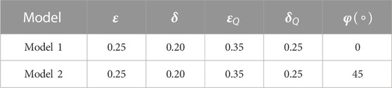
TABLE 1. Homogeneous model parameters for viscoacoustic wave propagation. Note that the reference velocity and quality factor are 2,400 m/s and 30, respectively, defined at the reference frequency of 1 Hz (i.e., ${\omega }_0=2\mathrm{\pi }$ rad/s).

FIGURE 1

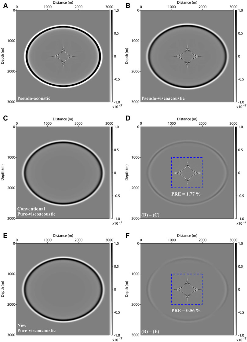
FIGURE 1. Wavefield snapshots at 0.45 s computed in Model 1. (A, B) are computed by the pseudo-acoustic and pseudo-viscoacoustic wave equations. (C, E) are computed by the conventional and our new pure-viscoacoustic wave equations. (D, F) are the differences between (B, C), and (B, E), respectively. The artifacts in the blue-line box are excluded in PRE calculations.

FIGURE 2

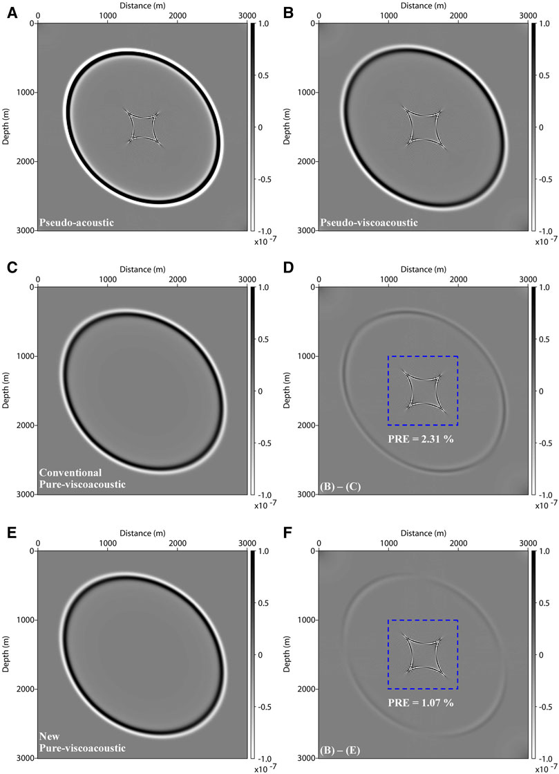
FIGURE 2. Wavefield snapshots at 0.45 s computed in Model 2. (A, B) are computed by the pseudo-acoustic and pseudo-viscoacoustic wave equations. (C, E) are computed by the conventional and our new pure-viscoacoustic wave equations. (D, F) are the differences between (B, C), and (B, E), respectively. The artifacts in the blue-line box are excluded in PRE calculations.

We also use the VTI (Model 1) and TTI (Model 2) homogeneous models to perform pure-viscoacoustic modeling with the decoupled forms. Figure 3 shows the corresponding wavefield snapshots computed in VTI and TTI attenuating media. In Figures 3A, C, each panel contains four wavefield snapshots, computed by the acoustic, dispersion-dominated, attenuation-dominated, and pure-viscoacoustic wave equations, respectively. Compared to the acoustic wavefield, the dispersion-dominated wavefield has a similar amplitude, but the phase is advancing. In contrast, the attenuation-dominated wavefield has significant attenuation on amplitude, while the traveltime is consistent with the acoustic result. Since the pure-viscoacoustic wave equation contains the amplitude attenuation and phase dispersion, both effects can be observed in the bottom-right corners of Figures 3A, C. Furthermore, we investigate the influence of different quality factors (Q = 200, 80, 30, and 15) on pure-viscoacoustic wave propagations. According to Figures 3B, D, more significant amplitude attenuation and phase distortion occur as quality factor Q decreases. A similar conclusion can be drawn from the extracted traces in Figure 4.

FIGURE 3

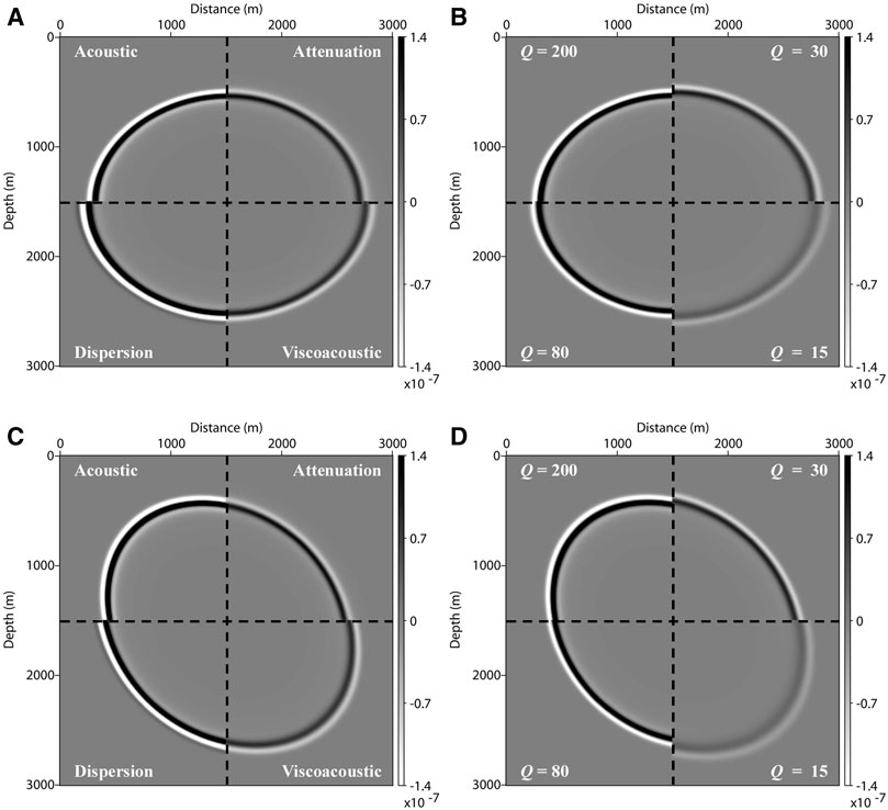
FIGURE 3. Viscoacoustic wavefield snapshots at 0.45 s computed in VTI (A, B) and TTI (C, D) homogeneous models. (A, C) are computed by the acoustic, dispersion-dominated, attenuation-dominated, and viscoacoustic wave equations. (B, D) are computed by the pure-viscoacoustic wave equation with Q = 200, 80, 30, and 15, respectively.

FIGURE 4

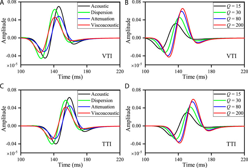
FIGURE 4. Trace comparisons computed in VTI (A, B) and TTI (C, D) homogeneous models. (A, C) are computed by the acoustic, dispersion-dominated, attenuation-dominated, and viscoacoustic wave equations. (B, D) are computed by the pure-viscoacoustic wave equation with Q = 200, 80, 30, and 15, respectively. Note that all traces are extracted at x = 1,000 m from seismic records.

3.2 Wavefield simulation in a two-layer model

The second example is a two-layer model (Figure 5). The first layer is a VTI medium, and the second layer is a TTI medium with a dip angle of 30°. The computational area is divided into 301 × 301 grids with a spatial interval of 10 m. The simulation duration and time step are 1.0 s and 1.0 ms, respectively. A Ricker wavelet with a peak frequency of 25 Hz is placed at (1,500 m, 1,200 m) to generate seismic vibrations. The reference frequency is 1 Hz. Figure 6 shows several wavefield snapshots at 0.5 s computed by the pseudo- (Figure 6B) and pure-viscoacoustic (Figure 6C) wave equations, respectively. In Figure 6B, some S-wave artifacts can be observed around the source (black arrow). Also, there are some converted S-wave artifacts (red arrow) in the figure, which are caused by the dip angle variations and may lead to numerical instability (white arrow). If there are no dip angle variations, the converted S-wave will disappear (Figure 6A). In contrast, the pure-viscoacoustic wave equation can fundamentally eliminate S-wave artifacts and improve simulation stability (Figure 6C). Figure 6D shows the wavefield difference between Figures 6B, C. The PRE of Figure 6D is as small as 2.32%. Meanwhile, Figures 6E, F show several trace comparisons extracted from Figures 6B, C at distances of 700 and 2,340 m. Both curves show a high level of agreement.

FIGURE 5

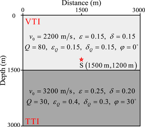
FIGURE 5. The two-layer model.

FIGURE 6

FIGURE 6. Viscoacoustic wavefield snapshots and extracted traces computed in the two-layer model. (A, B) are computed by the VTI and TTI pseudo-viscoacoustic wave equations. (C) is computed by the TTI pure-viscoacoustic wave equation. (D) is the difference between (B, C). (E, F) are extracted from (B, C) at x = 700 and 2,340 m, respectively. The artifacts in the blue-line box of (D) are excluded in PRE calculations.

3.3 Anisotropic Q-RTM in the modified BP gas chimney model

Finally, we use the modified BP gas chimney model (Figure 7) to perform anisotropic Q-RTM and examine the performance of the proposed method in anisotropic attenuating media. The model is divided into 398 × 181 grids with a spacing of 12 m in both directions. The simulation duration and time step are 3.0 s and 1 ms, respectively. The Ricker source with a peak frequency of 20 Hz is used to generate seismic vibrations. The reference frequency is 100 Hz. There are 67 shots evenly distributed at a depth of 12 m with an interval of 72 m in the horizontal direction. All wavefields are recorded by 398 receivers at the same depth as seismic sources during wavefield extrapolations. The anisotropic parameter and dip angle models are built using the following relations

$\begin{array}{cc}\epsilon =\frac{\left|v_0-2000\right|}{1000}\times 0.1+0.03,& \delta =\frac{\left|v_0-2000\right|}{1000}\times 0.06+0.05,\end{array}(27)$

$\begin{array}{ccc}{\epsilon }_Q=2\epsilon ,& {\delta }_Q=2.5\delta ,& \phi =60\epsilon +66.7\delta .\end{array}(28)$

FIGURE 7

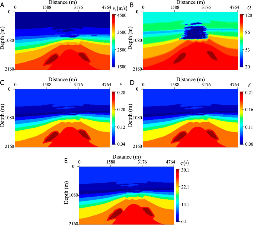
FIGURE 7. The modified BP gas chimney TTI model. (A) $v_0$. (B) Q. (C) $\epsilon$. (D) $\delta$. (E) $\phi$. (B–E) are built by Eqs. 27, 28, respectively. Note that the Q-dependent anisotropy parameters ${\epsilon }_Q=2\epsilon$ and ${\delta }_Q=2.5\delta$ are not shown here.

Figure 8 shows several wavefield snapshots of the 34th shot computed by the VTI and TTI pure-viscoacoustic wave equations, respectively. We can see that the proposed pure-viscoacoustic wave equation can simulate stable P-wave characteristics in complex anisotropic attenuating media. Compared with Figures 8A, B, some conspicuous differences can be observed between the wavefields computed by the VTI and TTI equations.

FIGURE 8

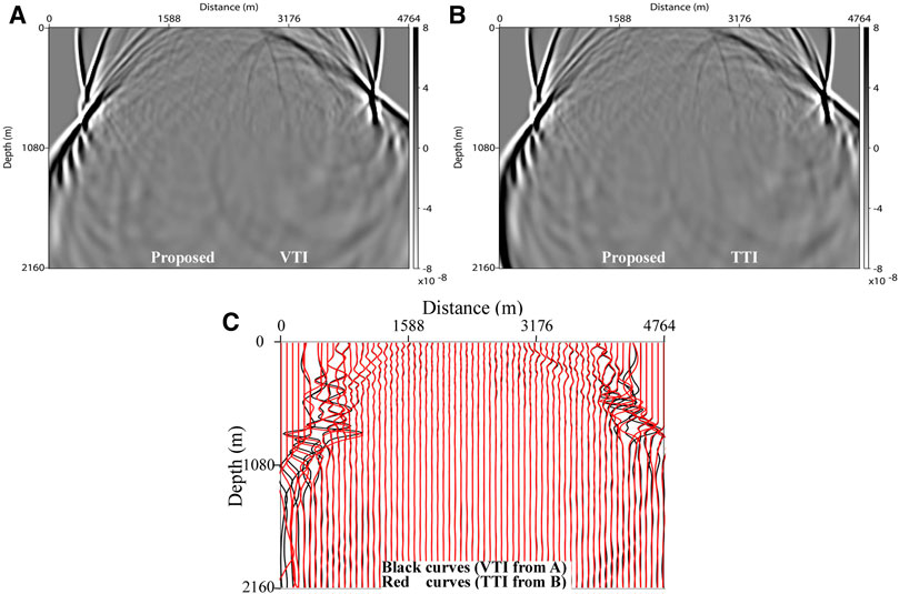
FIGURE 8. Wavefield snapshots at 1.3 s for the modified BP gas chimney model. (A, B) are computed by the VTI and TTI pure-viscoacoustic wave equations. (C) is the waveform comparison between (A, B). The source is located at (2,376 m, 12 m).

Based on the anisotropic Q-RTM workflow, we further use the modified BP gas chimney model to perform Q-RTM experiments. During the wavefield compensation, a low-pass filter with a cutoff frequency of 120 Hz is used to suppress high-frequency noise. Figure 9 shows several migrated images calculated by the anisotropic pure-acoustic (Figures 9A, B) and pure-viscoacoustic (Figures 9C, D) wave equations, respectively. Compared with the reference solution obtained by the acoustic RTM with lossless data, the acoustic RTM result using lossy data has obvious energy loss and resolution reduction, especially below the high-attenuation gas chimney. In contrast, the reflector amplitudes are well recovered in Figures 9C, D due to the compensated ability of the Q-RTM. Furthermore, trace comparisons (Figure 10) extracted from Figure 9 also give us a similar conclusion.

FIGURE 9

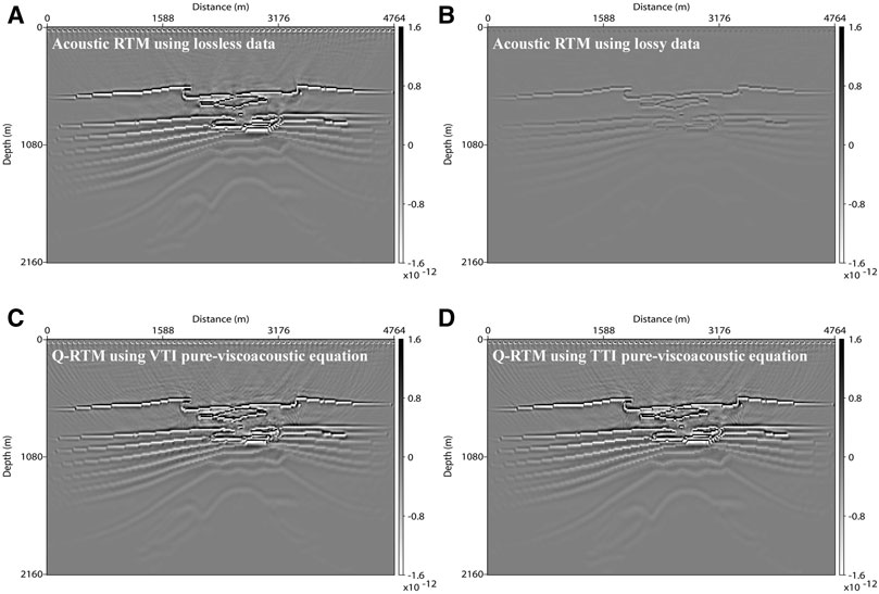
FIGURE 9. RTM images for the modified BP gas chimney model. (A, B) are computed by acoustic RTM using lossless and lossy data, respectively. (C, D) are the Q-RTM results computed by the VTI and TTI pure-viscoacoustic wave equations. A low-pass filter with a cutoff frequency of 120 Hz is used to suppress high-frequency noise.

FIGURE 10

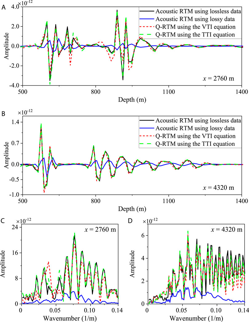
FIGURE 10. Trace comparisons (A, B) extracted from RTM images and their spectra (C, D).

3.4 The influence of anisotropy on Q-RTM and noisy data tests

We further use the modified BP gas chimney TTI model to investigate the influence of anisotropy on Q-RTM results. The parameters in numerical experiments include four groups: anisotropic quality factor and velocity (Figure 11A), isotropic quality factor (Figure 11B), isotropic velocity (Figure 11C), and isotropic quality factor and velocity (Figure 11D). Ignoring the anisotropy of the quality factor in Figure 11B reduces the resolution of the migrated image, especially in some strongly attenuating areas (see the blue box). However, ignoring the anisotropy of velocity in Figure 11C severely perturbs the Q-RTM results, causing many wavefields to converge incorrectly. Therefore, it has great meaning to develop an accurate pure-viscoacoustic wave equation for wave propagation and migration in anisotropic attenuating media.

FIGURE 11

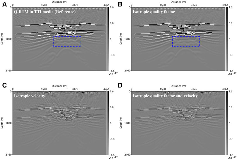
FIGURE 11. Pure-viscoacoustic Q-RTM profiles for the modified BP gas chimney model. (A) is computed with the anisotropic quality factor and velocity. (B) is computed with the isotropic quality factor. (C) is computed with the isotropic velocity. (D) is computed with the isotropic quality factor and velocity.

To evaluate the fidelity and anti-noise ability of the proposed method, we perform anisotropic Q-RTM tests with noisy data, obtained by adding Gaussian random noise with SNR = 10 and 5 dB. Figure 12 shows noisy data from the 34th shot. A low-pass filter with cutoff frequencies of 90 and 80 Hz is applied to suppress compensation instability. Overall, the migrated profiles in Figure 13 have very high resolution and the reflector amplitudes are well recovered although some weak noise can be observed. Compared with the Q-RTM result using clean data (Figure 9D), the energy of the migrated profiles in Figure 13 is partly reduced due to the low cutoff frequencies in the low-pass filtering.

FIGURE 12

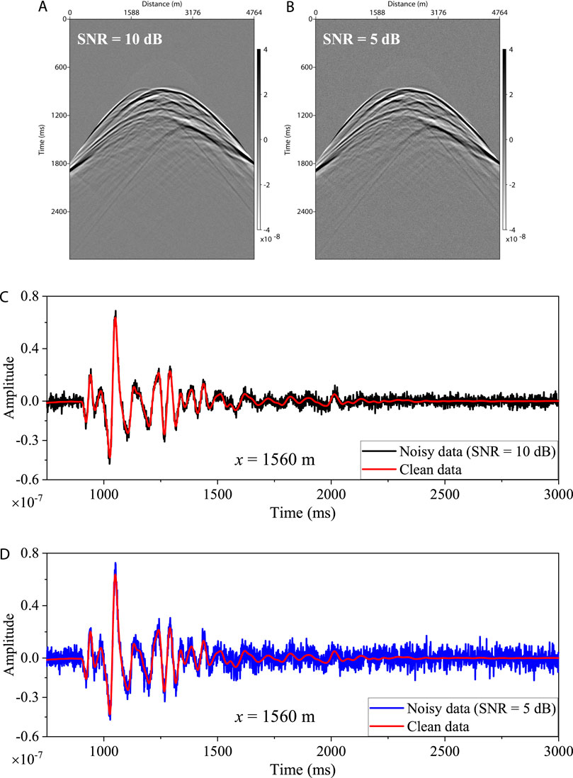
FIGURE 12. The 34th shot data for the BP gas chimney model. (A, B) are noisy data with SNR = 10 and 5 dB, respectively. (C) and (D) are the trace comparisons extracted at x = 1,560 m.

FIGURE 13

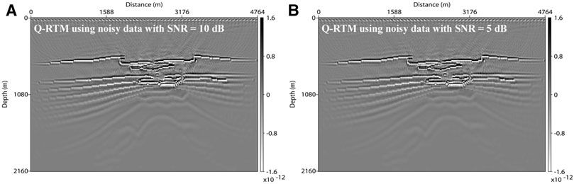
FIGURE 13. Anisotropic Q-RTM results using noisy data with (A) SNR = 10 dB and (B) SNR = 5 dB. A low-pass filter with cutoff frequencies of 90 and 80 Hz is used to suppress compensation instability in (A, B).

4 Conclusion

We derived a new pure-viscoacoustic wave equation by combining the complex dispersion relation and modified complex modulus in anisotropic attenuating media. Compared with the pseudo-viscoacoustic wave equation, the proposed pure-viscoacoustic equation can simulate stable P-wave characteristics in complex geological structures without S-wave artifacts. Since this new equation can simulate the decoupled amplitude attenuation and phase dispersion, we further use it to perform Q-RTMs and generate high-resolution images. Numerical experiments demonstrate the accuracy and robustness of the proposed method for pure-viscoacoustic wavefield simulations and migration imaging in transversely isotropic attenuating media.

Data availability statement

The original contributions presented in the study are included in the article/Supplementary Material, further inquiries can be directed to the corresponding author.

Author contributions

YZ: Methodology, Writing–original draft, Writing–review and editing. TC: Methodology, Supervision, Writing–review and editing.

Funding

The authors declare financial support was received for the research, authorship, and/or publication of this article. This research is financially supported by the National Key Research and Development Program of China under Grant 2021YFC2902003, the National Natural Science Foundation of China (NSFC) under Grant 42304123, a project funded by the Priority Academic Program Development of Jiangsu Higher Education Institutions, and the China Postdoctoral Science Foundation under Grant 2022M723384.

Acknowledgments

We would like to acknowledge the editors and reviewers, whose comments and suggestions significantly improved the manuscript.

Conflict of interest

The authors declare that the research was conducted in the absence of any commercial or financial relationships that could be construed as a potential conflict of interest.

Publisher’s note

All claims expressed in this article are solely those of the authors and do not necessarily represent those of their affiliated organizations, or those of the publisher, the editors and the reviewers. Any product that may be evaluated in this article, or claim that may be made by its manufacturer, is not guaranteed or endorsed by the publisher.

Supplementary material

The Supplementary Material for this article can be found online at: https://www.frontiersin.org/articles/10.3389/feart.2023.1290154/full#supplementary-material

References

Aki, K., and Richards, P. G. (2002). Quantitative seismology. United States: University Science Books.

Google Scholar

Alkhalifah, T. (2000). An acoustic wave equation for anisotropic media. Geophysics 65, 1239–1250. doi:10.1190/1.1444815

CrossRef Full Text | Google Scholar

Bai, T., and Tsvankin, I. (2016). Time-domain finite-difference modeling for attenuative anisotropic media. Geophysics 81, C69–C77. doi:10.1190/geo2015-0424.1

CrossRef Full Text | Google Scholar

Carcione, J. M. (2014). Wave fields in real media: wave propagation in anisotropic, anelastic, porous and electromagnetic media. Amsterdam, Netherlands: Elsevier.

Google Scholar

Carcione, J. M., Cavallini, F., Mainardi, F., and Hanyga, A. (2002). Time domain seismic modeling of constant-Q wave propagation using fractional derivatives. Pure Appl. Geophys. 159, 1719–1736. doi:10.1007/s00024-002-8705-z

CrossRef Full Text | Google Scholar

Carcione, J. M., Kosloff, D., and Kosloff, R. (1988). Wave propagation simulation in a linear viscoacoustic medium. Geophys. J. Int. 93, 393–401. doi:10.1111/j.1365-246x.1988.tb02010.x

CrossRef Full Text | Google Scholar

Carcione, J. M., Picotti, S., and Santos, J. E. (2012). Numerical experiments of fracture-induced velocity and attenuation anisotropy. Geophys. J. Int. 191, 1179–1191. doi:10.1111/j.1365-246X.2012.05697.x

CrossRef Full Text | Google Scholar

Chen, H., Zhou, H., Li, Q., and Wang, Y. (2016). Two efficient modeling schemes for fractional Laplacian viscoacoustic wave equation. Geophysics 81, T233–T249. doi:10.1190/geo2015-0660.1

CrossRef Full Text | Google Scholar

Chen, H., Zhou, H., and Rao, Y. (2020). An implicit stabilization strategy for Q-compensated reverse time migration. Geophysics 85, S169–S183. doi:10.1190/geo2019-0235.1

CrossRef Full Text | Google Scholar

Chichinina, T., Obolentseva, I., Gik, L., Bobrov, B., and Ronquillo-Jarillo, G. (2009). Attenuation anisotropy in the linear-slip model: interpretation of physical modeling data. Geophysics 74, WB165–WB176. doi:10.1190/1.3173806

CrossRef Full Text | Google Scholar

Da Silva, N. V., Yao, G., and Warner, M. (2019). Wave modeling in viscoacoustic media with transverse isotropy. Geophysics 84, C41–C56. doi:10.1190/geo2017-0695.1

CrossRef Full Text | Google Scholar

Duveneck, E., Milcik, P., and Bakker, P. M. (2008). Acoustic VTI wave equations and their application for anisotropic reverse-time migration. Seg. Tech. program Expand. Abstr., 2186–2190. doi:10.1190/1.3059320

CrossRef Full Text | Google Scholar

Fomel, S., Ying, L., and Song, X. (2013). Seismic wave extrapolation using lowrank symbol approximation. Geophys. Prospect. 61, 526–536. doi:10.1111/j.1365-2478.2012.01064.x

CrossRef Full Text | Google Scholar

Futterman, W. I. (1962). Dispersive body waves. J. Geophys. Res. 67, 5279–5291. doi:10.1029/jz067i013p05279

CrossRef Full Text | Google Scholar

Hao, Q., and Alkhalifah, T. (2017a). An acoustic eikonal equation for attenuating transversely isotropic media with a vertical symmetry axis. Geophysics 82, C9–C20. doi:10.1190/geo2016-0160.1

CrossRef Full Text | Google Scholar

Hao, Q., and Alkhalifah, T. (2017b). An acoustic eikonal equation for attenuating orthorhombic media. Geophysics 82, WA67–WA81. doi:10.1190/geo2016-0632.1

CrossRef Full Text | Google Scholar

Hao, Q., and Alkhalifah, T. (2019). Viscoacoustic anisotropic wave equations. Geophysics 84, C323–C337. doi:10.1190/geo2018-0865.1

CrossRef Full Text | Google Scholar

Hao, Q., and Greenhalgh, S. (2021). Nearly constant Q models of the generalized standard linear solid type and the corresponding wave equations. Geophysics 86, T239–T260. doi:10.1190/geo2020-0548.1

CrossRef Full Text | Google Scholar

Hao, Q., and Tsvankin, I. (2023). Thomsen-type parameters and attenuation coefficients for constant-Q transverse isotropy. Geophysics 88, C123–C134. doi:10.1190/geo2022-0575.1

CrossRef Full Text | Google Scholar

Hosten, B., Deschamps, M., and Tittmann, B. (1987). Inhomogeneous wave generation and propagation in lossy anisotropic solids: application to the characterization of viscoelastic composite materials. J. Acoust. Soc. Am. 82, 1763–1770. doi:10.1121/1.395170

CrossRef Full Text | Google Scholar

Kjartansson, E. (1979). Constant Q-wave propagation and attenuation. J. Geophys. Res. 84, 4737–4748. doi:10.1029/jb084ib09p04737

CrossRef Full Text | Google Scholar

Li, Q., Zhou, H., Zhang, Q., Chen, H., and Sheng, S. (2016). Efficient reverse time migration based on fractional Laplacian viscoacoustic wave equation. Geophys. J. Int. 204, 488–504. doi:10.1093/gji/ggv456

CrossRef Full Text | Google Scholar

Liu, F., Morton, S. A., Jiang, S., Ni, L., and Leveille, J. P. (2009). “Decoupled wave equations for P and SV waves in an acoustic VTI media,” in 79th annual international meeting (Expanded Abstracts: SEG), 2844–2848.

CrossRef Full Text | Google Scholar

Mu, X., Huang, J., Li, Z., Liu, Y., Su, L., and Liu, J. (2022). Attenuation compensation and anisotropy correction in reverse time migration for attenuating tilted transversely isotropic media. Surv. Geophys. 43, 737–773. doi:10.1007/s10712-022-09707-2

CrossRef Full Text | Google Scholar

Mu, X., Huang, J., Yang, J., Li, Z., and Ivan, M. S. (2021). Viscoelastic wave propagation simulation using new spatial variable-order fractional Laplacian. Bull. Seismol. Soc. Am. 112, 48–77. doi:10.1785/0120210099

CrossRef Full Text | Google Scholar

Qiao, Z., Chen, T., and Sun, C. (2022). Anisotropic attenuation compensated reverse time migration of pure qP-wave in transversely isotropic attenuating media. Surv. Geophys. 43, 1435–1467. doi:10.1007/s10712-022-09717-0

CrossRef Full Text | Google Scholar

Qiao, Z., Sun, C., and Tang, J. (2020). Modelling of viscoacoustic wave propagation in transversely isotropic media using decoupled fractional Laplacian. Geophys. Prospect. 68, 2400–2418. doi:10.1111/1365-2478.13006

CrossRef Full Text | Google Scholar

Qiao, Z., Sun, C., and Wu, D. (2019). Theory and modelling of constant-Q viscoelastic anisotropic media using fractional derivative. Geophys. J. Int. 217, 798–815. doi:10.1093/gji/ggz050

CrossRef Full Text | Google Scholar

Sun, J., and Zhu, T. (2018). Strategies for stable attenuation compensation in reverse-time migration. Geophys. Prospect. 66, 498–511. doi:10.1111/1365-2478.12579

CrossRef Full Text | Google Scholar

Thomsen, L. (1986). Weak elastic anisotropy. Geophysics 51, 1954–1966. doi:10.1190/1.1442051

CrossRef Full Text | Google Scholar

Wang, N., Xing, G., Zhu, T., Zhou, H., and Shi, Y. (2022). Propagating seismic waves in VTI attenuating media using fractional viscoelastic wave equation. J. Geophys. Res. Solid Earth 127, e2021JB023280. doi:10.1029/2021jb023280

CrossRef Full Text | Google Scholar

Wang, Y., Zhou, H., Chen, H., and Chen, Y. (2018). Adaptive stabilization for Q-compensated reverse time migration. Geophysics 83, S15–S32. doi:10.1190/geo2017-0244.1

CrossRef Full Text | Google Scholar

Wang, Y., Zhou, H., Zhao, X., Zhang, Q., and Chen, Y. (2019). Q-compensated viscoelastic reverse time migration using mode-dependent adaptive stabilization scheme. Geophysics 84, S301–S315. doi:10.1190/geo2018-0423.1

CrossRef Full Text | Google Scholar

Xing, G., and Zhu, T. (2019). Modeling frequency-independent Q viscoacoustic wave propagation in heterogeneous media. J. Geophys. Res. Solid Earth 112, 11568–11584. doi:10.1029/2019jb017985

CrossRef Full Text | Google Scholar

Yang, J., Huang, J., Zhu, H., Li, Z., and Dai, N. (2021). Viscoacoustic reverse time migration with a robust space-wavenumber domain attenuation compensation operator. Geophysics 86, S339–S353. doi:10.1190/geo2020-0608.1

CrossRef Full Text | Google Scholar

Yang, J., and Zhu, H. (2018). Viscoacoustic reverse time migration using a time-domain complex-valued wave equation. Geophysics 83, S505–S519. doi:10.1190/geo2018-0050.1

CrossRef Full Text | Google Scholar

Zeng, J., Stovas, A., and Huang, H. (2021). Anisotropic attenuation of stratified viscoelastic media. Geophys. Prospect. 69, 180–203. doi:10.1111/1365-2478.13042

CrossRef Full Text | Google Scholar

Zhang, Y., Chen, T., Liu, Y., and Zhu, H. (2023). High-temporal-accuracy viscoacoustic wave propagation based on k-space compensation and the fractional Zener model. Surv. Geophys. 44, 821–845. doi:10.1007/s10712-022-09765-6

CrossRef Full Text | Google Scholar

Zhang, Y., Liu, Y., and Xu, S. (2020). Arbitrary-order Taylor series expansion-based viscoacoustic wavefield simulation in 3D vertical transversely isotropic media. Geophys. Prospect. 68, 2379–2399. doi:10.1111/1365-2478.12999

CrossRef Full Text | Google Scholar

Zhang, Y., Liu, Y., Zhu, H., Chen, T., and Li, J. (2022). Modified viscoelastic wavefield simulations in the time domain using the new fractional Laplacian. J. Geophys. Eng. 19, 346–361. doi:10.1093/jge/gxac022

CrossRef Full Text | Google Scholar

Zhu, T. (2017). Numerical simulation of seismic wave propagation in viscoelastic-anisotropic media using frequency-independent Q wave equation. Geophysics 82, WA1–W10. doi:10.1190/geo2016-0635.1

CrossRef Full Text | Google Scholar

Zhu, T., and Bai, T. (2019). Efficient modeling of wave propagation in a vertical transversely isotropic attenuative medium based on fractional Laplacian. Geophysics 84, T121–T131. doi:10.1190/geo2018-0538.1

CrossRef Full Text | Google Scholar

Zhu, T., and Harris, J. M. (2014). Modeling acoustic wave propagation in heterogeneous attenuating media using decoupled fractional Laplacian. Geophysics 79, T105–T116. doi:10.1190/geo2013-0245.1

CrossRef Full Text | Google Scholar

Zhu, T., Harris, J. M., and Biondi, B. (2014). Q-compensated reverse-time migration. Geophysics 79, S77–S87. doi:10.1190/geo2013-0344.1

CrossRef Full Text | Google Scholar

Zhu, Y., and Tsvankin, I. (2006). Plane-wave propagation in attenuative transversely isotropic media. Geophysics 71, T17–T30. doi:10.1190/1.2187792

CrossRef Full Text | Google Scholar

Zhu, Y., Tsvankin, I., and Vasconcelos, I. (2007). Effective attenuation anisotropy of thin-layered media. Geophysics 72, D93–D106. doi:10.1190/1.2754185

CrossRef Full Text | Google Scholar