Tomographic reconstruction strategies for nondestructive testing with a commercial CT scanner

In this work, a framework was developed to access and process raw data from a commercial X-ray Computed Tomography (CT) scanner for research purposes. Our method requires vendor-provided binaries to convert the data to a readable format and also to remove the effect of proprietary beam hardening preprocessing. As a result, custom reconstruction techniques, including beam-hardening corrections algorithms, can be applied. Small region-of-interest CT imaging techniques and different backprojection algorithms were investigated to improve image quality (spatial resolution, noise) with an in-house iterative reconstruction algorithm. For a reconstruction matrix of 512 pixels × 512 pixels, processing times of approximately 2.5 s per slice were obtained using a set of 8 x GPUs. With this framework, high-quality images of high density samples (e.g., minerals) can be obtained with reduced truncation-induced blurring, free of artifacts stemming from the reconstruction process and reduced beam-hardening artifacts.

1 Introduction

X-ray Computed Tomography (CT) is nowadays ubiquitous in medicine for diagnosis, treatment planning, and treatment response purposes. This technology is also increasingly used for non-medical purposes in many fields, including archaeology, industrial metrology Kruth et al. (2011); De Chiffre et al. (2014), geology Fortin et al. (2013); Kibria et al. (2014); Périard et al. (2016), the timber industry, biology Mizutani and Suzuki (2012), industrial x-ray inspection and aviation security Ying et al. (2006). It provides several advantages such as: (i) non-destructive imaging and (ii) high spatial and density resolution Kaick and Delorme (2005).

When compared to a microCT scanner, a medical CT scanner can present some advantages such as faster scanning time and the possibility to scan large samples Hipsley et al. (2020). There are some drawbacks however in using a device that was developed for scanning the human anatomy, including artifacts for high-density samples, photon starvation problems and lower spatial resolution Barrett and Keat (2004). At INRS Eau Terre Envinronnement in Quebec City, the Multidisciplinary Laboratory of CT-Scan for Natural Resources and Civil Engineering is equipped with a modified medical CT scanner, mounted on rails and using a custom CT table, which allows scanning long samples, such as sediment cores Fortin et al. (2013).

In clinical CT scanners, raw acquisition data are stored as sinograms and are typically processed by proprietary methods, notably to reduce beam hardening artifacts in reconstructed images, which are often obtained with filtered backprojection algorithms (e.g., FDK) Feldkamp et al. (1984). Raw sinograms are relatively large from a storage perspective and are typically not kept on the long term, as opposed to reconstructed images which are normally sent to a database. Even though it is possible to archive sinograms, their proprietary format typically prevents users from reading them. The sinograms could also be preprocessed (e.g., calibration, beam-hardening correction), and in this respect might not truly represent raw CT data, i.e., measures of attenuation along a ray. In some cases, including for research purposes, it is desirable to access this raw attenuation data to use custom tomographic reconstruction algorithms, including iterative ones where physics priors can be considered. In this class of algorithms, the image output is obtained by optimizing an specific objective function Matenine et al. (2015c), which usually requires the computation of several forward- and backprojection steps Geyer et al. (2015).

Several methods can be used for forward- and backprojection in tomographic reconstruction, and the choice is typically driven by a trade-off between image quality, from a human observer perspective, accuracy in terms of quantitative density reconstruction, and processing time. For the ray-driven backprojection, the accumulation process in each voxel (the process on which the attenuation values for each ray are accumulated onto a set of voxels, which represent the 3D volume of the object) depends on the number of rays, where some voxels might not be intersected at all, giving rise to artifacts. A known solution, which increases computation time, is to define detector sub-pixels, or to upsample the projection data, so that the number of rays are multiplied by a constant factor. Likewise, better accuracy with voxel-driven backprojection methods is achieved by dividing a voxel into smaller sub-voxels Zhuang et al. (1994). These methods can be advantageously implemented on highly-parallel GPUs through different approaches, allowing faster execution times Matenine et al. (2015b); Park et al. (2015).

Previous work have shown the importance of the forward projection model on image quality for iterative reconstruction algorithms Hahn et al. (2016). Adding the forward- and backprojection models as reconstruction parameters makes the assessment of different techniques more complex, as each method comes with several degrees of freedom.

We have developed a framework where an in-house iterative algorithm can be used to reconstruct images based on genuinely raw attenuation data. First, the sinogram data in proprietary format are converted through the use of binaries provided by the manufacturer. The conversion generates useable sinogram data along with associated geometrical data. These data are then used to perform the reconstruction with the iterative algorithm OSC-TV (ordered subsets convex algorithm with total variation technique) Matenine (2011). In this work, two backprojection techniques were evaluated in terms of their impact on image features: a Siddon-based (ray-driven) Siddon (1985) and a bilinear interpolation (voxel-driven) approach. A technique used to reconstruct regions-of-interest with this class of algorithms was also analyzed Ziegler et al. (2008), as they allow for reduced truncation artifacts caused by objects outside the reconstruction matrix. Finally, a custom beam-hardening correction (BHC) algorithm can be applied on raw data, in combination with the aforementioned techniques.

2 Background

2.1 OSC-TV

The Ordered Subset Convex (OSC) iterative reconstruction algorithm (IR) is based on the maximization of the log-likelihood:

$L\left(\mu \right)=-{\displaystyle \sum _i}\left(b_i{e}^{-t_i}+Y_i{t}_i\right),(1)$

where μ is the image estimate, b_i is the photon count for the detector index i in the absence of a sample, t_i is the total attenuation t_i = ∑_jl_ijμ_j, and Y_i is the transmitted data, where the index j represents the voxels intersected by the ray going from the source to the detector i. For a photon-counting detector, the transmission is giving by:

$Y_i=b_i{e}^{-t_i}.(2)$

The CT Scanner uses energy-integrating detectors (EIDs), so b_i represents the total energy read by the detector. Even though Y_i will not strictly follow a Poisson distribution, this model can be considered a good approximation Man et al. (2001).

The maximum of the objective function defined by Eq. 1 is obtained via ordered subsets convex (OSC) expectation-maximization algorithm Matenine et al. (2015a). In this case, the convergence is accelerated by using subsets of projections for the forward- and the backprojection step of the algorithm, given by the following expression:

${\mu }_{s+1}^{\left(n\right)}={\mu }_s^{\left(n\right)}+{\mu }_s^{\left(n\right)}\frac{{\sum }_{i\in S\left(s\right)}{l}_{ij}\left[{\overline{y_i}}^{\left(n\right)}-Y_i\right]}{{\sum }_{i\in S\left(s\right)}{l}_{ij}{t}_i^{\left(n\right)}{\overline{y_i}}^{\left(n\right)}},(3)$

where n is the reconstruction iteration number, $\overline{y_i}$ is the estimated photon count, s is the index of the subset and S(s) is a well defined function that generates for each selected group of projections the subsets of rays Matenine (2011); Di Schiavi Trotta et al. (2022). A high number of subsets is used to accelerate the reconstruction, whereas this value should be reduced at every iteration in order to decrease bias Beekman and Kamphuis (2001); Sidky et al. (2006).

A full OSC iteration step is completed when all the projections have been used to update the expected value of the attenuation μ⁽ⁿ⁾. Once this step finishes, the image is regularized within the image space by the total variation minimization technique (TV) Matenine et al. (2011).

2.2 Forward- and backprojection techniques

In the OSC-TV algorithm, the estimated image is forward- and backprojected several times, depending on the number of iterations and subsets, which are determined empirically Matenine et al. (2015b).

In this work, the estimated image is forward projected using Siddon’s algorithm Siddon (1985), which is a ray-driven (RD) technique that can be efficiently implemented on the GPU Matenine et al. (2015b). Backprojection was performed in this work with two techniques: (i) voxel-driven with bilinear interpolation (VD) Zhuang et al. (1994) or (ii) ray-driven. For the former, a mismatch occurs from mathematical perspective as the backprojector is not the transpose operator of the forward projector. Such mismatch pair combinations are known to cause convergence issues and artifacts on the reconstructed image Zeng and Gullberg (2000), but was explored nonetheless here (Section 3.2).

In the voxel-driven backprojection with bilinear interpolation, the center of each voxel is projected on the detector and the reading corresponds to the weighted sum of the four neighboring pixels (the position is calculated relative to the detector pixel centers).

For a ray-based backprojection, the detector readings are smeared back across the image. The voxels that are incremented in this process depend on the ray path from the source to the detector reading. Typically, a finite number of rays are defined (e.g., one ray per detector element). In this approach, depending on the angle between rays and the voxel size, some voxels might not be traversed by a given ray at all, or they are under-utilized, for the intersection length is negligible. This problem is not unique to the backprojection; it is also present in the forward projection in different techniques (e.g., Siddon, Joseph’s method, and bilinear interpolation) Hahn et al. (2016). Hence, some voxels of the reconstruction matrix grid might play no role in modeling some projections, degrading the accuracy of the forward projection model.

A multiray ray-driven approach for forward- and backprojection can be used to address the fundamental problem of unintersected voxels with ray-based techniques Zhuang et al. (1994). For that, the detector elements are evenly divided into smaller sub-pixels, where each ray now intersect their respective centers. For a 1 × 1 detector geometry, hence, one sub-pixel, there is one ray path per element, for a 2 × 2 geometry, 4 ray paths per bin, and so on. For the parallel implementation of the algorithm on the GPU through CUDA (Compute Unified Device Architecture), with our framework, the number of threads per block was defined by the maximum number of voxels traversed by any ray, which assigns each ray to a GPU thread. Multiple rays are obtained by a loop over the subpixels in a thread.

3 Materials and methods

3.1 Working with proprietary format

For this work, a Siemens SOMATOM Definition AS+ 128 scanner was used. This CT scanner is capable of performing acquisitions with up to 4,608 projections in a single rotation, through the use of the flying focal spot (FFS) technology (with four focal point locations). The detector grid is made of 736 pixels x 64 pixels, with a detector size in the axial direction of 0.6 mm (other configurations are possible, as for example, a detector size in the longitudinal axis z of 1.2 mm and a detector grid of 736 pixels x 32 pixels). The X-ray tube can be operated in the range of 70–140 kVp. This platform is used for several non-medical applications, including material characterization with dual-energy techniques Fortin et al. (2013); Larmagnat et al. (2019); Martini et al. (2021); Di Schiavi Trotta et al. (2022).

The process of using raw data from this medical CT scanner is illustrated in Supplementary Figure S1. A vendor-provided calibration table is used for acquisitions to cancel any vendor-specific beam hardening corrections (detector calibration is still applied). The raw data is stored in the host system and copied to a different machine for archiving purposes, along with calibration data. These raw data, free of vendor-specific beam hardening corrections, can be read with vendor-provided binaries. These genuinely raw data (except for detector calibration), can thereafter be used in custom reconstruction algorithms designed to handle corrections from first principles, notably through dual-energy approaches Di Schiavi Trotta et al. (2022) (Supplementary Figure S1).

3.2 Convergence of OSC-TV for a virtual phantom: matched and mismatched projector/backprojector pair

A virtual phantom (Figure 1) was used to assess the algorithmic convergence of our reconstruction methods in different situations, including one with a mismatched projector/backprojector pair (unmatched), namely, Siddon-based ray-driven/voxel-driven with bilinear backprojection. The matched case uses a Siddon-based ray-driven for both the forward- and the backprojection. The numerical phantom represents a 25.2 cm water cylinder and 9 cylinder rods of distinct materials, each one with a diameter of 2.4 cm. The virtual phantom dimensions are: 512 pixels × 512 pixels, with a pixel size in x- and y-direction of 0.6 mm (transaxial plane), and 1.0 mm in the z-direction (longitudinal direction). The X-ray absorption property of the phantom, defined by the linear attenuation coefficient, was retrieved from the NIST XCOM database Suplee (2009).

FIGURE 1

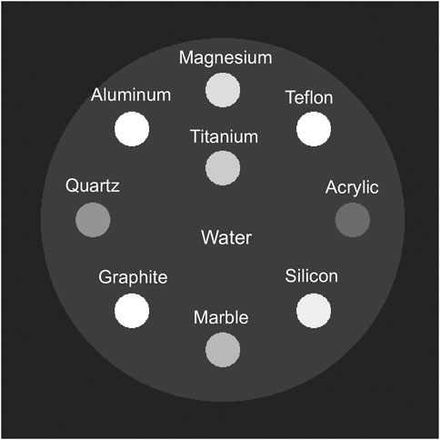
FIGURE 1. Virtual phantom representing a cylinder of water (diameter of 25.2 cm) and 9 cylindrical rods (diameter of 2.4 cm).

A noise-free monoenergetic step-and-shoot acquisition of the virtual phantom at 83 keV was simulated by using the geometry of the medical CT scanner Siemens SOMATOM Definition AS+ 128: two flying focal spots, a detector grid with dimensions 736 pixels × 32 pixels, with a detector pixel size in z of 1.2 mm (longitudinal direction), and 2,304 projections.

The convergence trend of the reconstruction was tuned by the reconstruction parameters: number of iterations, number of subsets, final number of subsets, and initial image; regularization parameters also play an important role in decreasing the overall noise and controlling the spatial resolution: number of gradient steps and strength of regularization Matenine et al. (2015b).

A high number of subsets, equivalent to one quarter of the number of projections, can be used to achieve faster calculations Beekman and Kamphuis (2001). The number of subsets can be progressively reduced in order to reduce the bias in the final image.

Different combinations of reconstruction parameters were used to assess the convergence for both the matched and the unmatched cases: 9 iterations for all cases; 576 (1/4 projections) and 1152 (1/2 projections) subsets. A total of 4 reconstructions were performed (2 × 2), to sample the convergence parameter space, with the regularization constant and gradient steps fixed at 0.02 and 20, respectively. This combination in OSC-TV is known to enhance the spatial resolution of realistic features Matenine et al. (2015b), when compared to smoother combinations, such as setting the regularization constant to 0.2 Matenine et al. (2011).

In order to assess the convergence of the OSC-TV with a virtual phantom, the map of the percent error for each pair of pixels was used, defined by:

$\text{percent\hspace{0.17em}error\hspace{0.17em}}\left(\%\right)=\frac{x^{\mathit{pred}}-x^{\mathit{true}}}{x^{\mathit{true}}}\times 100\%,(4)$

where x^true is the ground truth image, which for the virtual phantom is the tabulated (NIST) linear attenuation coefficient of each material at 83 keV. This particular energy was chosen as it coincides with the effective energy of the X-ray spectral response of the system at a tube voltage of 140 kVp Di Schiavi Trotta et al. (2022). Finally, x_pred is the reconstructed image obtained with OSC-TV.

The root-mean-square deviation (RMSE), defined as:

$\mathrm{R}\mathrm{M}\mathrm{S}\mathrm{E}=\sqrt{\frac{{\sum }_{i=0}^{n_{\mathit{voxels}}-1}{\left(x_i^{\mathit{true}}-x_i^{\mathit{pred}}\right)}^2}{n_{\mathit{voxels}}}},(5)$

where n_voxels is the number of voxels, was used to evaluate the convergence of the reconstruction of the virtual phantom. For a single slice, the RMSE is computed for each material of the virtual phantom as well as for all the materials (including water). Voxels at the edges are also included in the calculation, which may increase the RMSE due to partial-volume averaging and blurring on material boundaries.

The mean absolute percent error (MAPE) from a certain region of the image can be obtained from:

$\text{MAPE\hspace{0.17em}}\left(\%\right)=\frac{1}{N}{\displaystyle \sum _{i=1}^N}\frac{|x_i^{\mathit{pred}}-x_i^{\mathit{true}}|}{x_i^{\mathit{true}}}\times 100\%,(6)$

where N is the number of pixels, and its used to evaluate how close a reconstructed image of a homogeneous sample is to the correspondent tabulated linear attenuation coefficient evaluated at the effective energy of the associated X-ray spectrum.

The beam-hardening ratio (BHR), defined as Ying et al. (2006); Di Schiavi Trotta et al. (2022):

$BHR=\frac{\left|P_{\mathit{edge}}-P_{\mathit{center}}\right|}{P_{\mathit{edge}}}\times 100\%,(7)$

is used to evaluate cupping artifacts on reconstructed images of both preprocessed, and neutral projections.

3.3 Scanning protocols

In order to compare the Siemens reconstruction algorithm with our in-house code, 6 samples were scanned (see Figure 2): a water phantom, (a) an aluminum cylinder, (b) a jar of water with an oblique aluminum bar, two mineral samples, namely, (c) chalcopyrite, and (d) almandine, and one rock sample, a homogeneous medium to coarse-grained sandstone, henceforth referred to as sandstone (Table 2).

FIGURE 2

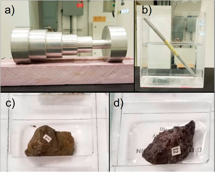
FIGURE 2. Scanned samples: (A) aluminum cylinder, (B) jar of water with oblique aluminum cylinder (Water+Al), (C) chalcopyrite, (D) almandine. The water phantom and the sandstone used can be seen in Figures 3A, D of our previous work Di Schiavi Trotta et al. (2022).

Different scan protocols were used depending on the sample size and X-ray absorption properties. The sequential acquisition mode was used due to its simplicity over the helicoidal mode for in-house iterative reconstruction algorithms (see Table 1).

TABLE 1

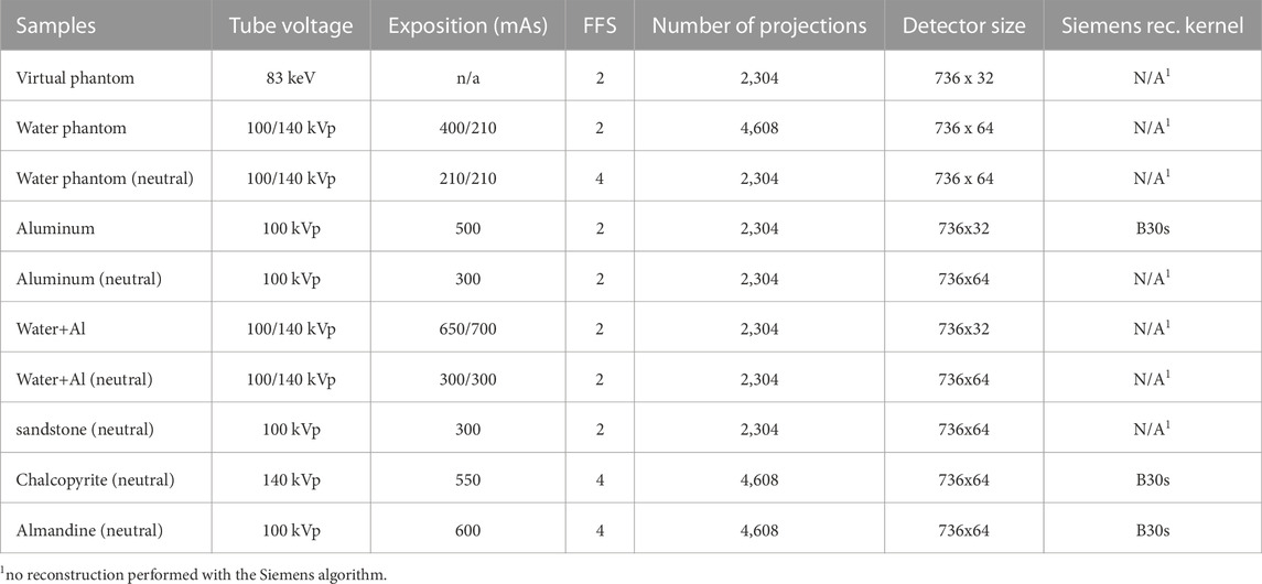
TABLE 1. Acquisition parameters for the samples using the Siemens SOMATOM Definition AS+ 128, including the number of FFS used in the scanning process. Neutral projections are obtained by neutralizing proprietary beam-hardening preprocessing.

The water phantom was scanned with two different tube voltages, 100 kVp and 140 kVp, with and without the proprietary BHC preprocessing. The case without the proprietary BHC is henceforth defined as neutralized projections (neutral). This allows us to both calibrate the system (see Section 3.4) and to assess the impact of the preprocessing on the reconstructed image.

A homogeneous aluminum cylinder with a diameter of 75 mm was also scanned at 100 kVp, with and without proprietary BHC, to assess beam-hardening artifacts, where a custom beam-hardening correction algorithm was also applied. A jar was filled with water and a small aluminum cylinder was submerged obliquely and scans at 100 and 140 kVp were also performed, with and without BHC preprocessing, to analyse the profile of the projections at a specific angle, so the effect of beam-hardening preprocessing on different materials can be appreciated on the projection.

The three smaller samples, sandstone, almandine, and chalcopyrite, were scanned with neutral BHC. Their size allows us to explore truncation artifacts, which can be reduced through the iterative reconstruction of a region-of-interest, and the effect of different backprojection techniques. For chalcopyrite, ray-driven backprojection with multiple rays per detector was also used, as well as the custom beam-hardening correction algorithm. This highly attenuating sample allow us to appreciate the correction of cupping artifacts.

3.4 Conversion calibration

Tomographic reconstructions performed by the OSC-TV algorithm are inherently in units of linear attenuation (cm⁻¹), while the ones obtained with the Siemens algorithm are in Hounsfield units (HU). The relation between these quantities is given by:

$\mu =\left(\frac{HU}{1000}+1\right)\times {\mu }_{\mathit{water}}(8)$

hence, given the attenuation of water, one can easily calculate the attenuation map from the images in HU units. Reconstructions of the water phantom, at 100 kVp and 140 kVp, were performed with OSC-TV, and the mean value in a 200 pixels × 200 pixels square ROI of each case was calculated. The average of the results obtained from the preprocessed projections provides an estimation of the μ_water value used in the proprietary conversion process. This value is independent of the tube voltage, for the projections are always normalized for water, so HU is always close to 0 (proprietary preprocessing of raw data). Thus, the images provided by the Siemens system in HU units can now be easily converted to attenuation values through Eq. 8. This conversion allows us to compare the accuracy of the reconstructions obtained with each method.

3.5 Reconstruction of raw data using OSC-TV

Numerical experiments have guided the choice of the reconstruction parameters used in the real samples. All samples were reconstructed with 9 iterations and 228 subsets, with 29 final number of subsets (1/10th), except for the smaller samples, i.e., chalcopyrite and almandine. These small samples were reconstructed with the same number of iterations, but with 72 subsets and 8 final number of subsets (see Table 2).

TABLE 2

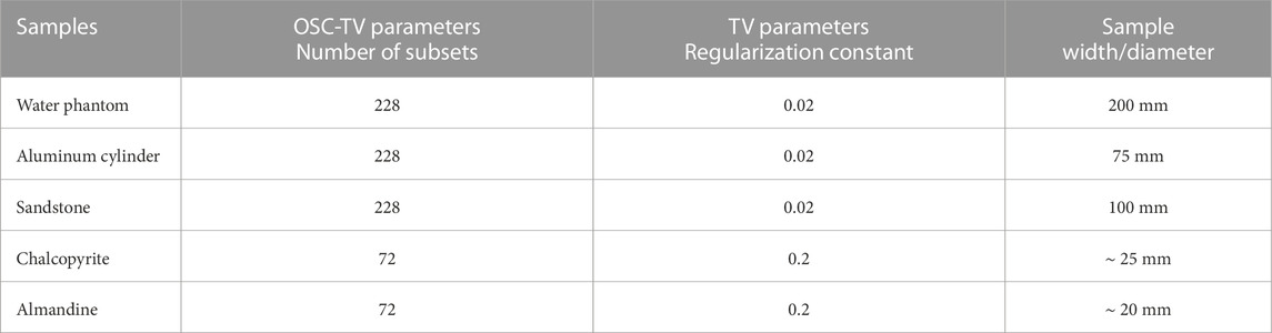
TABLE 2. Reconstruction parameters for the samples with OSC-TV and its variations. All samples are reconstructed with 9 iterations.

As we aim to compare the Siemens images with the images obtained with our in-house code (OSC-TV), voxel sizes were set to the same value in both cases. At the same time, truncation artifacts are to be avoided, hence, a larger grid was used in some cases (water phantom and aluminum cylinder) so all scanned objects, including the CT table, are present in the reconstruction matrix grid Ziegler et al. (2008) (see Table 3). A modified technique to reconstruct a region-of-interest through an iterative reconstruction algorithm (IR ROI) was applied to mitigate artifacts on reconstructions with small field-of-view (FOV) (see Section 3.6).

TABLE 3

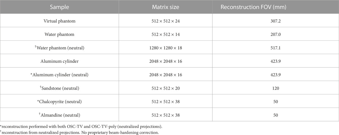
TABLE 3. Reconstruction matrix size and FOV defined for the OSC-TV algorithm.

3.6 Small ROI reconstruction

The voxel size is ultimately constrained in our algorithms by the fact that all objects that participate in the X-ray absorption process should be included in the FOV to mitigate truncation artifacts. Hence, even if small samples are scanned (e.g., 5 cm, 10 cm, etc.), the entire FOV (50 cm) shall be reconstructed so that the CT table is included in the reconstruction matrix. For that, either a larger voxel size is used or a larger grid size (e.g., 1024 × 1024, 2048 × 2048, etc.), where the latter increases substantially the reconstruction time.

In order to remove the effect of the CT table in imaging small samples (small FOV), a technique based on the work of Ziegler et al. (2008) was implemented to mitigate truncation artifacts. The modified technique works as follows: (i) a reconstruction using the iterative code, OSC-TV, with a voxel size of 0.977 × 0.977 × 1.2 mm³, with a reconstruction matrix size of 512 pixels × 512 pixels is performed. In this step, the voxel-driven backprojection with bilinear interpolation was chosen. This reconstruction is henceforth defined as OSC-TV low (low resolution). With such a configuration, a reconstruction of the entire FOV is obtained (500 mm). In order to accelerate this step, a fraction of the projections were used, either 1/4 or 1/8 depending on the scan configuration, totaling 576 projections; (ii) a square ROI containing the object in the reconstructed image is set to zero; (iii) this image is now forward projected (FP) with GPU-acceleration using Siddon’s algorithm Siddon (1985); (iv) these projections are then subtracted from the original sinogram; (v) the region outside the ROI in this sinogram is set to zero to further reduce truncation artifacts on the final reconstruction; (vi) the result is finally reconstructed with the IR algorithm. Differently from what was proposed in Ziegler et al. (2008), no transition region was used, as the main objective of the applications of such technique was to remove the table interference, not to select a ROI within the scanned sample itself.

3.7 Custom beam-hardening correction

With proprietary beam-hardening corrections neutralized, one is able to apply custom methods to mitigate such artifacts and take into account the properties of various materials for the correction (such as dense minerals and metals). Here, the method developed by Trotta et al. (2022) Di Schiavi Trotta et al. (2022), OSC-TV-poly, was applied to show how images with reduced artifacts can be obtained (see Table 4). The calibration curve, bowtie filter model, X-ray spectra and detector response were the same as in the cited paper for the case where the tube voltage was set at 140 kVp Di Schiavi Trotta et al. (2022). For the 100 kVp case, a new calibration curve was developed with the correspondent X-ray spectrum and detector response (Supplementary Figure S2).

TABLE 4

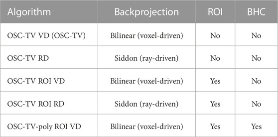
TABLE 4. Acronyms of the reconstruction strategies based on OSC-TV. Siddon-based ray-driven forward projection (RD) is used in all algorithms, while voxel-driven backprojection with bilinear interpolation (VD) is employed in all algorithms except OSC-TV RD, and OSC-TV ROI RD.

Table 4 summarizes acronyms used to refer to implementation strategies and the different algorithm combinations (forward projection, backprojection, IR ROI technique, BHC).

Iterative reconstruction algorithms are computationally intensive Després and Jia (2017), hence, reconstructions with OSC-TV were performed on a NVIDIA DGX™ A100, which is equipped with 8 x NVIDIA A100 Tensor Core GPUs with 40 GB of RAM, with 6912 cores each. For benchmarking purposes, some reconstructions were performed with 8 GPUs.

In our MultiGPU approach, at each subset Matenine et al. (2015b), the different projections are processed (estimated image is forward- and backprojected) simultaneously by the different GPUs. The result is then copied from all the GPUs to the main GPU, and finally, the image is updated. After all subsets are processed, the image is regularized using only the main GPU.

4 Results

4.1 Convergence of OSC-TV for a virtual phantom: matched and mismatched projector/backprojector pair

The visual representation of the convergence of the OSC-TV algorithm for the virtual phantom in terms of the number of subsets and for the matched/unmatched cases is depicted in Figure 3, while the RMSE of each material as a function of these parameters are shown in Figure 4.

FIGURE 3

FIGURE 3. Percent error maps of the reconstruction of the virtual phantom with OSC-TV in terms of the number of subsets. Two cases are shown: matched (ray-driven/ray-driven) and unmatched projector/backprojector pair (ray-driven/voxel-driven), reconstructed with 9 iterations and initial number of subsets of 576 and 1152.

FIGURE 4

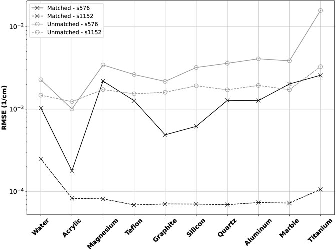
FIGURE 4. Convergence of OSC-TV for each material in the virtual phantom in terms of the RMSE.

RMSE is in the order of 10^–3 for all materials in the virtual phantom even when 576 subsets are used (9 iterations), except for titanium, which presents an important density and atomic number.

4.2 Calibration: Water phantom

An average value μ_water = 0.192 cm⁻¹ was obtained from the measurements in the central slice of the water phantom images, reconstructed with OSC-TV, from preprocessed projections, at 100 kVp and 140 kVp. These measurements allow the scaling from HU to linear attenuation coefficient (see Figure 5).

FIGURE 5

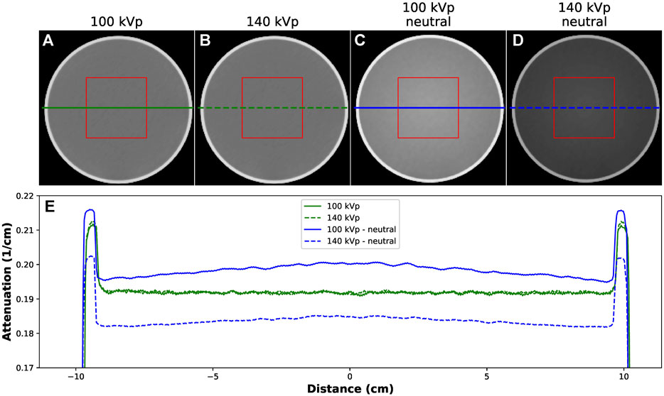
FIGURE 5. Water phantom reconstructed with OSC-TV from different acquisition protocols: (A) 100 kVp with preprocessing, (B) 140 kVp with preprocessing, (C) 100 kVp neutral, (D) 140 kVp neutral, (E) plot of the line profile. Window: [0.17:0.22]. In (A) and (B) the proprietary preprocessing is present, so attenuation values are the same. For (D) and (E), where the preprocessing was removed, attenuation values reflect the X-ray spectra, and capping artifacts are observed due to the bowtie filter.

4.3 Proprietary preprocessing

The first projection of four different acquisitions of the jar of water with an aluminum bar (Water+Al) are shown in Figure 6, as well as the respective line profiles. In (a) and (b), it is shown how the proprietary preprocessing for beam-hardening correction normalized all projection values for water, despite the different tube voltage. On the other hand, in (c) and (d), where also the pairs 100 kVp and 140 kVp were used, projection values for water are different, and so reflect more closely the X-ray spectrum properties of each tube voltage. Furthermore, the projection values for aluminum are also more distant, showing that such corrections affect different materials.

FIGURE 6

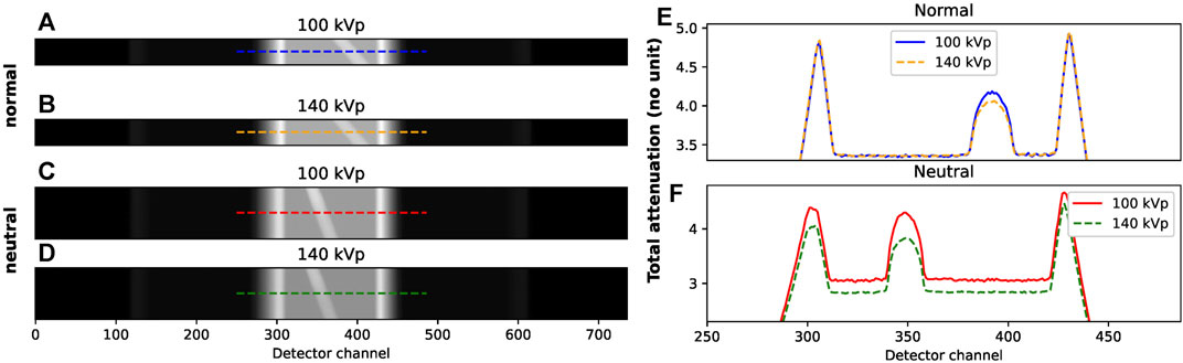
FIGURE 6. Jar of water with oblique aluminum bar (Water+Al): (A, B) projection of Water+Al for the angle 270^o at 100 kVp and 140 kVp, (C, D) projection of Water+Al for the angle 270^o at 100 kVp and 140 kVp, where a different detector grid is used and proprietary BHC is neutralized, (E) line profile of Water+Al projections, 100 kVp and 140 kVp, (F) line profile of Water+Al projections, 100 and 140 kVp, with proprietary BHC neutralized. For (C) and (D), where BHC preprocessing is removed, total attenuation reflects X-ray spectra, and the X-ray absorption properties of the scanned materials. Window [0.00:5.00] (no unit).

4.4 Small ROI reconstruction: OSC-TV ROI

The importance of the backprojection technique for artifact mitigation and the IR ROI technique for removing truncation artifacts is shown in Figure 7. In (a) and (b), the CT table was not included in the reconstruction matrix, hence, the IR algorithm, through the forward- and backprojection, tries to reproduce the raw projection by updating an image where no table is being reconstructed. Artifacts appear in the reconstructed image, identified as the four bright spots on the image and 2 lines joining them, reflecting the presence of the table in projection data (but not in the reconstructed FOV). It is worth noting that the setup uses a custom table capable of supporting heavy samples but associated with a higher attenuation than a medical one. Secondly, in (c), the image is reconstructed using ray-driven backprojection (Siddon based) and the IR ROI technique.

FIGURE 7

FIGURE 7. Sandstone scanned at 100 kVp, reconstructed with OSC-TV: (A) ray-driven backprojection (RD), (B) voxel-driven backprojection with bilinear backprojection (VD), (C) RD backprojection and ROI technique, (D) VD backprojection and ROI technique. Window [0.5:0.6] cm⁻¹. In (A) and (B) the CT couch outside the FOV produces artifacts in the reconstructed image (cross-like pattern), while in (C) and (D) such effect is removed, since the table was removed from projection data.

In Figure 8, the reconstruction of a small sample of almandine (5 cm) is shown with different techniques: (a) Siemens with the B30s kernel (smooth); (b) OSC-TV with ray-driven backprojection; (c) OSC-TV with voxel-driven backprojection; (d): OSC-TV with the ROI IR technique, and voxel-driven backprojection. As a smooth kernel was selected for the Siemens reconstruction, the OSC-TV images appear sharper (better spatial resolution).

FIGURE 8

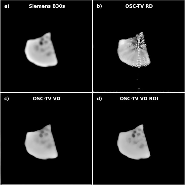
FIGURE 8. Almandine scanned at 100 kVp: (A) reconstruction with Siemens algorithm (kernel B30s), (B) reconstruction performed with OSC-TV and ray-driven (RD) backprojection, (C) reconstruction performed with OSC-TV and voxel-driven (VD) backprojection, (D) reconstruction performed with OSC-TV, voxel-driven (VD) backprojection and region-of-interest strategy, Window [1.0:1.8] cm⁻¹.

The effect of increasing the number of rays per detector bin with a ray-driven approach regarding the artifacts in the images is visible with the chalcopyrite samples (see Supplementary Figure S3). Voxel-driven backprojection with no sub-voxels (1x1) is sufficient to avoid the artifact present in the case of the ray-driven backprojection with no sub-pixels (1x1), where it requires 16x16 rays per detector in order to reduce the artifact.

4.5 Comparing Siemens and OSC-TV: custom beam-hardening corrections

Images reconstructed with the Siemens algorithm (kernel B30s), OSC-TV VD (OSC-TV), and OSC-TV-poly, is shown in Figure 9, along with the plot of line profiles.

FIGURE 9

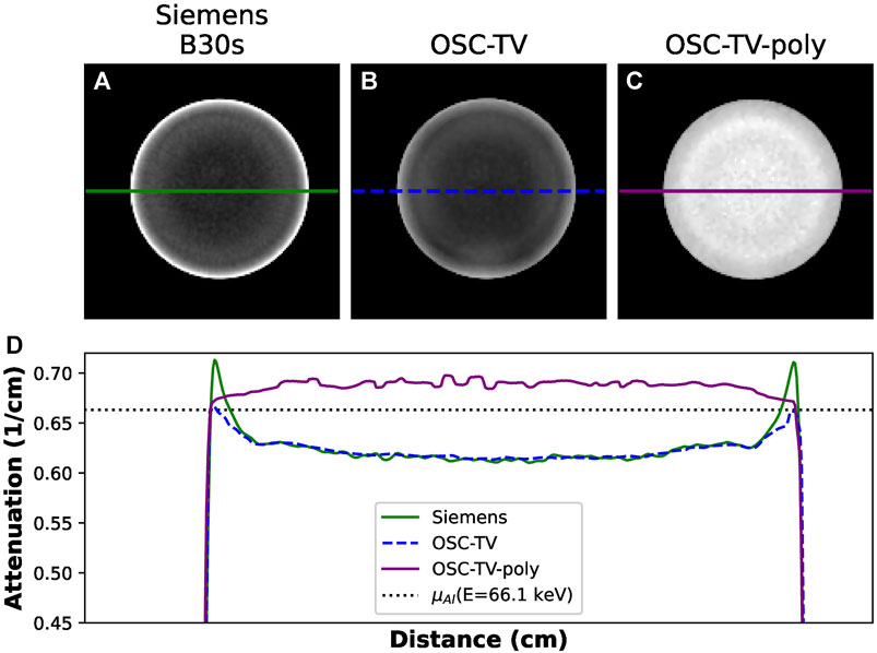
FIGURE 9. Aluminum cylinder scanned at 100 kVp, from preprocessed and neutral projections: (A) reconstruction with the Siemens algorithm (preprocessed, kernel B30s), (B) reconstruction performed with OSC-TV (preprocessed), (C) reconstruction performed with OSC-TV-poly (neutral), (D) plot of the line profiles of Siemens, OSC-TV, and OSC-TV-poly. Window [0.60:0.70] cm⁻¹.

Applying OSC-TV-poly (modeling beam hardening in the reconstruction algorithm), along with ROI reconstruction strategies and the voxel-driven backprojection (VD), cupping artifacts, even in a small and dense object, were reduced when compared to the ordinary OSC-TV and Siemens images (see Figure 10). In (b) and (c), where IR ROI and voxel-driven technique were applied, the reconstructed image is not deteriorated by truncation artifacts due to the CT table and artifacts from the ray-driven backprojection implementation.

FIGURE 10

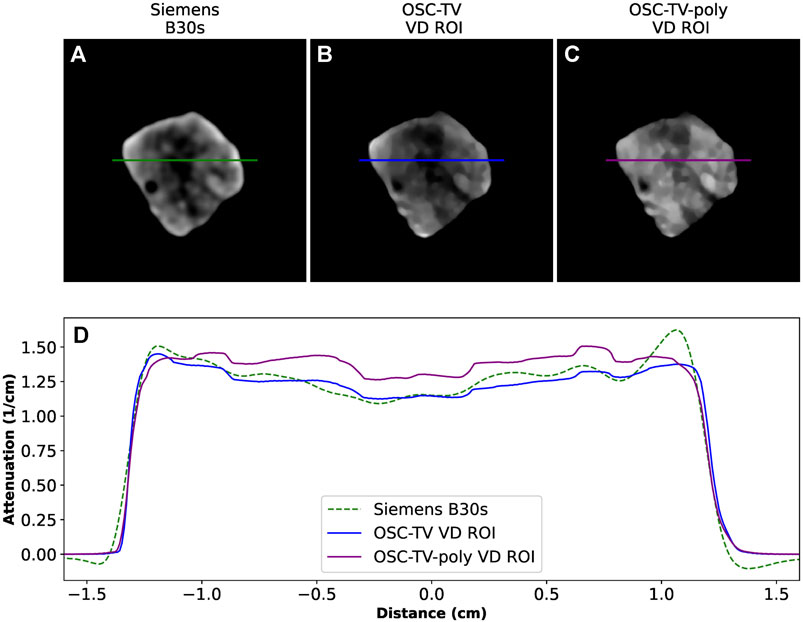
FIGURE 10. Chalcopyrite scanned at 140 kVp: reconstructions with (A) Siemens algorithm (kernel B30s), (B) OSC-TV ROI algorithm, (C) OSC-TV-poly ROI, (D) corresponding line profiles. Window [1.1:1.7] cm⁻¹.

4.6 Processing time

Reconstruction time may vary substantially depending on the reconstruction algorithm (as well as reconstructions parameters) and the forward- and backprojection methods Geyer et al. (2015), even when using GPU acceleration Després and Jia (2017). The iterative reconstruction of a region-of-interest requires an additional reconstruction (OSC-TV low) and an additional forward projection (FP) step before a final reconstruction of the ROI is performed (OSC-TV RD ROI or OSC-TV VD ROI). These extra steps increase the overall processing time (OSC-TV low + FP + OSC-TV ROI RD/VD), as outlined below.

Two samples were used to compare reconstruction times, sandstone (FOV=12 cm) and chalcopyrite (FOV=5 cm), where the latter uses twice the number of projections, and an initial number of subsets of 72, instead of 288. Reconstruction grid sizes are 512 pixels × 512 pixels × 20 pixels for the sandstone and 512 pixels × 512 pixels × 38 pixels for chalcopyrite. The initial reconstruction of the entire FOV (OSC-TV low) takes 6 s for all the samples, while the forward projection time takes approximately 1 s for these two cases. Hence, less than 7 extra seconds are required to perform the reconstruction of a ROI, as summarized in Table 5.

TABLE 5

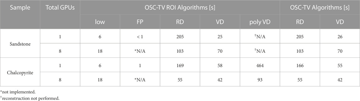
TABLE 5. Comparison of reconstruction time using a NVIDIA A100 Tensor Core GPU 40 GB (1 and 8 GPUs). Sandstone and chalcopyrite samples are reconstructed with 9 iterations, an initial number of subsets of 288 and 72, with a grid size of 512 × 512 × 20 and 512 × 512 × 38, respectively.

5 Discussion

Regarding the assessment of the convergence of the OSC-TV algorithm using the virtual phantom, depicted in Figure 3, it becomes evident that 576 subsets is insufficient (1/4 of the number of projections) even when 9 iterations are performed, giving rise to beam-hardening-like artifacts, which are more important in the matched case. As those images were reconstructed from monochromatic projections (83 keV), such artifacts were not expected. By increasing the number of subsets to 1152 (half the number of projections), such artifacts are decreased, and the convergence for the rods (denser materials) are more acceptable, where RMSE is an order of magnitude lower for some materials (see Figure 4), mainly for the matched case. Materials with high-density and atomic number tend to present higher RMSE, and hence, slower convergence. The RMSE of water on the other hand is highly affected by the materials rods (transition zones between water and rods).

Moreover, the percent error for these materials is lower than 0.05% in these cases, which can be considered high accuracy in many applications, such as in material characterization and identification Landry et al. (2013); Bourque et al. (2014); Azevedo et al. (2016); Paziresh et al. (2016); Martini et al. (2021), where errors are much higher due to beam-hardening artifacts. Hence, this set of parameters could be employed for reconstructing homogeneous samples; it was observed that a high number of subsets is required when reconstructing highly attenuating samples. Otherwise, the convergence rate is low and many iterations are required.

Even though a mismatched projector/backprojector pair was used in this work, no convergence problem was observed in any studied case (RMSE decreases as the number of iterations increases), except for acrylic in the unmatched case, which presents higher RMSE when a higher number of initial subsets is used. Moreover, the use of such combinations in iterative reconstruction algorithms (e.g., ASIRT, additive simultaneous iterative reconstruction techniques), has been shown to present more accurate reconstructed images when compared to the ones produced with matched operators Guedouar and Zarrad (2010). Other works have demonstrated otherwise, where the coupling between such operators is crucial for achieving more accuracy for this class of algorithms Zeng and Gullberg (2000). Meanwhile, other suggests that the use of mismatched projector/backprojector pairs can achieve solutions closer to the true image, when compared to the matched case Zeng (2019).

Regarding the measurements conducted in the water phantom for the conversion calibration, as beam-hardening preprocessing was not neutralized, the mean value is independent of the tube voltage (so HU=0 for all tube voltages), and so can be used to convert HU to cm⁻¹ regardless of the tube voltage and either or not the beam-hardening preprocessing was used on the target projection (see Supplementary Table S1, where tabulated linear attenuation values of water for the effective energy of the X-ray spectra correspondents to the tube voltages of 100 kVp and 140 kVp are also shown). In summary, with beam-hardening preprocessing, pixel values for water are always the same, so the same μ_water is used by the manufacturer to perform the conversion from linear attenuation coefficient to HU for all tube voltages.

For the case where neutralized projections were used, and reconstruction performed with OSC-TV, distinct mean attenuation values were obtained, with a higher value for the 100 kVp setting, hence, reflecting the X-ray absorption properties of the water phantom (Supplementary Table S1 reports tabulated vs. measured μ values). A capping artifact is observed on neutralized images (Figure 5), which is caused by the bowtie filter Di Schiavi Trotta et al. (2022).

The neutralization of the preprocessing step, depicted in Figures 5, 6, therefore allows the application of custom energy-dependent beam-hardening correction techniques, since data directly reflect the X-ray spectrum and the absorption properties of the scanned materials Alvarez and Macovski (1976); Man et al. (2001); Ying et al. (2006); Champley and Bremer (2014); Azevedo et al. (2016); Paziresh et al. (2016); Di Schiavi Trotta et al. (2022).

Due to the small size of the sandstone and the small voxel sizes used in the respective tomographic reconstructions (Figure 7), the separation of adjacent rays is large compared to the voxel size Hahn et al. (2016), so some voxels are missed during the raytracing in the backprojection. As not all voxels are incremented by the correspondent detector read, more artifacts arise, producing a poor quality image, however, with no truncation artifacts Trotta et al. (2022), whereas (b) suffers from both artifacts. Finally, in (d), both IR ROI and voxel-driven with bilinear interpolation are combined. These two techniques are capable of mitigating both artifacts: truncation and streaks caused by an insufficient number of rays used during backprojection.

For the tomographic reconstructions of almandine (Figure 8), image (b) suffers from the inherent problem of the ray-driven backprojection, where some voxels are not properly incremented by the backprojection and Moiré patterns arise at the center of the image. The contrast in image (c) is degraded compared to image (d), the result of the CT couch being smeared across the reconstructed volume. From a qualitative point of view, such effect can be observed on the black spots of image (d), which are more contrasted. The white line observed at the edges of the sample in (a) is less important on the OSC-TV reconstructions in general (b,c, and d), indicating less beam-hardening artifacts.

When comparing properties of images obtained with proprietary (Siemens) and in-house (OSC-TV) algorithms (Figure 9), one can note that in the aluminum cylinder, even though proprietary beam-hardening correction is applied to all projections, cupping artifacts are still present, because such corrections are optimized for water. However, such artifacts are less important in the OSC-TV image, with lower pixel values at the edges. This effect is further reduced with OSC-TV-poly, that reconstructs the aluminum cylinder from neutral projections. The BHR is reduced from 14%, obtained with Siemens, to 8% with OSC-TV, and then to only 3% with OSC-TV-poly.

Reference attenuation values for aluminum, evaluated at the estimated effective energy of the 100 kVp beam, are represented by the dotted line in Figure 9, which are closer to the ones reconstructed by OSC-TV-poly. The mean absolute percent error evaluated for this line profile for the proprietary (Siemens) reconstruction is 6.2%, for OSC-TV is 6.0%, and for OSC-TV poly is 3.7%. Hence, this algorithm has the potential to reconstruct images closer to the effective energy of the beam.

Given the variety of geological samples and associated properties (e.g., shape, porosity, density, mixtures of materials with low/high atomic numbers), it is not trivial to find generic regularization parameters. From our observations, we found the a value 0.2 (20 gradient steps) yields high-quality images in terms of spatial resolution and noise for small FOV (small samples). On the other hand, samples that are highly heterogeneous yield better images with lower regularization parameters, hence the choice of 0.02 (and 20 gradient steps). It is difficult to define a quantitative quality metrics and some experiments with reconstruction parameters are recommended.

In regard to the evaluation of the processing times for the two presented cases, sandstone (FOV=12 cm) and chalcopyrite (FOV=5 cm), the reconstruction with the ray-based technique took longer than the voxel-driven one, mainly for the sandstone, which was approximately 8x slower. That can be explained by the higher number of subsets used in the reconstruction, which implies more memory transfers between CPU and GPU, and between GPUs, and more calls to the CUDA kernels responsible for the forward- and the backprojection.

By using multiple GPUs in parallel, similar computation time was observed for these techniques. It is clear with the voxel-driven technique that the poor speed gain is related to the limitation of memory bandwidth, as the data of all the GPUs have to be transferred to the main GPU after a subset is processed, increasing processing time.

In some cases, as for the OSC-TV low, the use of multiple GPUs actually increases the computation time. This counter-intuitive result is due to the problem being limited by memory bandwidth capacity, not by computing power capacity (time taken to copy data to GPU devices longer than actual calculations).

The use of more rays per detector bin has the potential to decrease streak artifacts typical of ray-driven projectors. However, adequate strategies must be employed to reap the full potential of GPUs, for example, by coalescing operations so that one thread block can be used to compute multiple adjacent rays Chou et al. (2011). For our approach, which assigns one ray (which is divided into sub-rays for defining sub-pixels) for each CUDA thread, it took 670 min for 256 rays (16 x 16), against only 2 min and 46 s when compared to a single ray.

Finally, for the chalcopyrite (512 pixels × 512 pixels × 38 pixels), on which both ROI and BHC are applied, it takes 8 times longer to perform the reconstruction when compared to the case where no beam-hardening corrections are applied, totalling 8 min. However, when a set of 8 GPUs are used, the difference drops to less than 1 min. This processing time could be much higher (e.g., a few hours) if a larger grid (e.g., 2048 pixels × 2048 pixels) were used to compensate for the voxel size and the truncation-induced artifacts Di Schiavi Trotta et al. (2022), showing the importance of the IR ROI technique for both mitigating artifacts, and reducing processing time.

6 Conclusion

Noise-free simulation results showed that, in our framework, the use of a ray-driven matched projector/backprojector pair outperforms the unmatched voxel-driven backprojector, with a ray-driven forward-projector.

The framework presented in this work, relying on raw data obtained through vendor-provided binaries, allows the development of custom tomographic reconstruction approaches, adapted to non-medical use of CT scanner (e.g., dense samples), capable of producing images with better quantitative properties. This framework was used here to evaluate a small ROI reconstruction method where truncation artifacts are mitigated, and also to assess the relative merit of two backprojection methods (ray-driven and voxel-driven), with a ray-driven forward-projector. Faster processing times were obtained for the unmatched case, which provided sharper and artifact-free images of small samples, when compared to the matched case.

These strategies, when combined with a custom BHC, yield better images of high-density samples (with reduced cupping when compared to the ones provided by the manufacturer and adapted for human imaging). Further processing acceleration is obtained with the ROI technique and the use of multiple GPUs, when compared to former works.

Data availability statement

The raw data supporting the conclusion of this article will be made available by the authors, without undue reservation.

Author contributions

LD: Conceptualization, Data curation, Formal Analysis, Investigation, Methodology, Software, Validation, Visualization, Writing–original draft, Writing–review and editing. DM: Software, Writing–review and editing. YL: Writing–review and editing. MM: Resources, Writing–review and editing. KS: Writing–review and editing, Software. MR: Writing–review and editing, Investigation. PL: Investigation, Writing–review and editing. PF: Investigation, Writing–review and editing, Conceptualization, Funding acquisition, Methodology, Resources, Supervision. PD: Software, Writing–review and editing, Conceptualization, Data curation, Funding acquisition, Investigation, Methodology, Project administration, Resources, Supervision.

Funding

The author(s) declare financial support was received for the research, authorship, and/or publication of this article. This research was supported by the Sentinel North program of Université Laval, made possible by the Canada First Research Excellence Fund. This work was also supported by a grant from Fonds de recherche du Québec - Nature et technologies (2018-PR-206076), and in part by the NSERC CREATE in Responsible Health and Healthcare Data Science.

Acknowledgments

We would like to thaank Jérôme Landry and Pascal Bourgault for the essential help in setting the foundation of the algorithms used in this work, and Stéphanie Larmagnat for providing rock samples.

Conflict of interest

KS is an employee of Siemens Healthcare GmbH, Forchheim, Germany.

The remaining authors declare that the research was conducted in the absence of any commercial or financial relationships that could be construed as a potential conflict of interest.

Publisher’s note

All claims expressed in this article are solely those of the authors and do not necessarily represent those of their affiliated organizations, or those of the publisher, the editors and the reviewers. Any product that may be evaluated in this article, or claim that may be made by its manufacturer, is not guaranteed or endorsed by the publisher.

Supplementary material

The Supplementary Material for this article can be found online at: https://www.frontiersin.org/articles/10.3389/feart.2023.1287059/full#supplementary-material

References

Alvarez, R. E., and Macovski, A. (1976). Energy-selective reconstructions in X-ray computerised tomography. Phys. Med. Biol. 21, 733–744. doi:10.1088/0031-9155/21/5/002

PubMed Abstract | CrossRef Full Text | Google Scholar

Azevedo, S. G., Martz, H. E., Aufderheide, M. B., Brown, W. D., Champley, K. M., Kallman, J. S., et al. (2016). System-independent characterization of materials using dual-energy computed tomography. IEEE Trans. Nucl. Sci. 63, 341–350. doi:10.1109/TNS.2016.2514364

CrossRef Full Text | Google Scholar

Barrett, J. F., and Keat, N. (2004). Artifacts in CT: recognition and avoidance. Radiographics 24, 1679–1691. doi:10.1148/rg.246045065

PubMed Abstract | CrossRef Full Text | Google Scholar

Beekman, F. J., and Kamphuis, C. (2001). Ordered subset reconstruction for x-ray CT. Phys. Med. Biol. 46, 1835–1844. doi:10.1088/0031-9155/46/7/307

PubMed Abstract | CrossRef Full Text | Google Scholar

Bourque, A. E., Carrier, J.-F., and Bouchard, H. (2014). A stoichiometric calibration method for dual energy computed tomography. Phys. Med. Biol. 59, 2059–2088. doi:10.1088/0031-9155/59/8/2059

PubMed Abstract | CrossRef Full Text | Google Scholar

Champley, K. M., and Bremer, T. (2014). Efficient and accurate correction of beam hardening artifacts. Livermore, CA (United States): Lawrence Livermore National Lab. Tech. Rep. LLNL-CONF-649613.

Google Scholar

Chou, C.-Y., Chuo, Y.-Y., Hung, Y., and Wang, W. (2011). A fast forward projection using multithreads for multirays on GPUs in medical image reconstruction. Med. Phys. 38, 4052–4065. doi:10.1118/1.3591994

PubMed Abstract | CrossRef Full Text | Google Scholar

De Chiffre, L., Carmignato, S., Kruth, J. P., Schmitt, R., and Weckenmann, A. (2014). Industrial applications of computed tomography. CIRP Ann. 63, 655–677. doi:10.1016/j.cirp.2014.05.011

CrossRef Full Text | Google Scholar

Després, P., and Jia, X. (2017). A review of GPU-based medical image reconstruction. Phys. Med. 42, 76–92. doi:10.1016/j.ejmp.2017.07.024

PubMed Abstract | CrossRef Full Text | Google Scholar

Di Schiavi Trotta, L., Matenine, D., Martini, M., Stierstorfer, K., Lemaréchal, Y., Francus, P., et al. (2022). Beam-hardening corrections through a polychromatic projection model integrated to an iterative reconstruction algorithm. NDT E Int. 126, 102594. doi:10.1016/j.ndteint.2021.102594

CrossRef Full Text | Google Scholar

Feldkamp, L. A., Davis, L. C., and Kress, J. W. (1984). Practical cone-beam algorithm. J. Opt. Soc. Am. A 1, 612. doi:10.1364/JOSAA.1.000612

CrossRef Full Text | Google Scholar

Fortin, D., Francus, P., Gebhardt, A. C., Hahn, A., Kliem, P., Lisé-Pronovost, A., et al. (2013). Destructive and non-destructive density determination: method comparison and evaluation from the Laguna Potrok Aike sedimentary record. Quat. Sci. Rev. 71, 147–153. doi:10.1016/j.quascirev.2012.08.024

CrossRef Full Text | Google Scholar

Geyer, L. L., Schoepf, U. J., Meinel, F. G., Nance, J. W., Bastarrika, G., Leipsic, J. A., et al. (2015). State of the art: iterative CT reconstruction techniques. Radiology 276, 339–357. doi:10.1148/radiol.2015132766

PubMed Abstract | CrossRef Full Text | Google Scholar

Guedouar, R., and Zarrad, B. (2010). A comparative study between matched and mis-matched projection/back projection pairs used with ASIRT reconstruction method. Nucl. Instrum. Methods Phys. Res. Sect. A Accel. Spectrom. Detect. Assoc. Equip. 619, 225–229. doi:10.1016/j.nima.2010.02.077

CrossRef Full Text | Google Scholar

Hahn, K., Schöndube, H., Stierstorfer, K., Hornegger, J., and Noo, F. (2016). A comparison of linear interpolation models for iterative CT reconstruction. Med. Phys. 43, 6455–6473. doi:10.1118/1.4966134

PubMed Abstract | CrossRef Full Text | Google Scholar

Hipsley, C. A., Aguilar, R., Black, J. R., and Hocknull, S. A. (2020). High-throughput microCT scanning of small specimens: preparation, packing, parameters and post-processing. Sci. Rep. 10, 13863. doi:10.1038/s41598-020-70970-7

PubMed Abstract | CrossRef Full Text | Google Scholar

Kaick, G. v., and Delorme, S. (2005). Computed tomography in various fields outside medicine. Eur. Radiol. Suppl. 15, d74–d81. doi:10.1007/s10406-005-0138-1

CrossRef Full Text | Google Scholar

Kibria, G., Hossain, M. S., and Ali, A. (2014). Innovative approach to soil characterization using X-ray computed Tomography. Atlanta, GE: CT, 1557–1566. doi:10.1061/9780784413272.152

CrossRef Full Text | Google Scholar

Kruth, J. P., Bartscher, M., Carmignato, S., Schmitt, R., De Chiffre, L., and Weckenmann, A. (2011). Computed tomography for dimensional metrology. CIRP Ann. 60, 821–842. doi:10.1016/j.cirp.2011.05.006

CrossRef Full Text | Google Scholar

Landry, G., Seco, J., Gaudreault, M., and Verhaegen, F. (2013). Deriving effective atomic numbers from DECT based on a parameterization of the ratio of high and low linear attenuation coefficients. Phys. Med. Biol. 58, 6851–6866. doi:10.1088/0031-9155/58/19/6851

PubMed Abstract | CrossRef Full Text | Google Scholar

Larmagnat, S., Des Roches, M., Daigle, L.-F., Francus, P., Lavoie, D., Raymond, J., et al. (2019). Continuous porosity characterization: metric-scale intervals in heterogeneous sedimentary rocks using medical CT-scanner. Mar. Petroleum Geol. 109, 361–380. doi:10.1016/j.marpetgeo.2019.04.039

CrossRef Full Text | Google Scholar

Man, B. D., Nuyts, J., Dupont, P., Marchal, G., and Suetens, P. (2001). An iterative maximum-likelihood polychromatic algorithm for CT. IEEE Trans. Med. Imaging 20, 999–1008. doi:10.1109/42.959297

PubMed Abstract | CrossRef Full Text | Google Scholar

Martini, M., Francus, P., Di Schiavi Trotta, L., and Després, P. (2021). Identification of common minerals using stoichiometric calibration method for dual-energy CT. Geochem. Geophys. Geosystems 22, e2021GC009885. doi:10.1029/2021GC009885

CrossRef Full Text | Google Scholar

Matenine, D. (2011). Reconstruction itérative sur matériel graphique en tomodensitométrie. Master’s thesis. Montréal, QC: Université de Montréal.

Google Scholar

Matenine, D., Goussard, Y., and Després, P. (2015a). “Evaluation of the OSC-TV reconstruction algorithm for optical cone-beam computed tomography,” in Proceedings of the IUPESM 2015 world congress on medical physics and biomedical engineering. Editor D. Jaffray (Springer International Publishing), 51, 236–239.

CrossRef Full Text | Google Scholar

Matenine, D., Goussard, Y., and Després, P. (2015b). GPU-accelerated regularized iterative reconstruction for few-view cone beam CT. Med. Phys. 42, 1505–1517. doi:10.1118/1.4914143

PubMed Abstract | CrossRef Full Text | Google Scholar

Matenine, D., Hissoiny, S., and Després, P. (2011). “Gpu-accelerated few-view ct reconstruction using the osc and tv techniques,” in Proceedings of the 11th International Meeting on Fully Three-Dimensional Image Reconstruction in Radiology and Nuclear Medicine, Germany (Potsdam, Germany: Potsdam).

Google Scholar

Matenine, D., Mascolo-Fortin, J., Goussard, Y., and Després, P. (2015c). Evaluation of the OSC-TV iterative reconstruction algorithm for cone-beam optical CT. Med. Phys. 42, 6376–6386. doi:10.1118/1.4931604

PubMed Abstract | CrossRef Full Text | Google Scholar

Mizutani, R., and Suzuki, Y. (2012). X-ray microtomography in biology, 43. Oxford, England: Micron, 104–115. doi:10.1016/j.micron.2011.10.002

CrossRef Full Text | Google Scholar

Park, H.-G., Shin, Y.-G., and Lee, H. (2015). A fully GPU-based ray-driven backprojector via a ray-culling scheme with voxel-level parallelization for cone-beam CT reconstruction. Technol. Cancer Res. Treat. 14, 709–720. doi:10.7785/tcrt.2012.500429

PubMed Abstract | CrossRef Full Text | Google Scholar

Paziresh, M., Kingston, A. M., Latham, S. J., Fullagar, W. K., and Myers, G. M. (2016). Tomography of atomic number and density of materials using dual-energy imaging and the Alvarez and Macovski attenuation model. J. Appl. Phys. 119, 214901. doi:10.1063/1.4950807

CrossRef Full Text | Google Scholar

Périard, Y., Gumiere, S. J., Long, B., Rousseau, A. N., and Caron, J. (2016). Use of X-ray CT scan to characterize the evolution of the hydraulic properties of a soil under drainage conditions. Geoderma 279, 22–30. doi:10.1016/j.geoderma.2016.05.020

CrossRef Full Text | Google Scholar

Siddon, R. L. (1985). Fast calculation of the exact radiological path for a three-dimensional CT array. Med. Phys. 12, 252–255. doi:10.1118/1.595715

PubMed Abstract | CrossRef Full Text | Google Scholar

Sidky, E. Y., Kao, C.-M., and Pan, X. (2006). Accurate image reconstruction from few-views and limited-angle data in divergent-beam CT. X-ray Sci. Tech. 14, 119–139. doi:10.48550/arXiv.0904.4495

CrossRef Full Text | Google Scholar

Suplee, C. (2009). XCOM: photon cross sections database.

Google Scholar

Trotta, L. D. S., Matenine, D., Martini, M., Lemaréchal, Y., Francus, P., and Després, P. (2022). “On the use of voxel-driven backprojection and iterative reconstruction for small ROI CT imaging,” in 7th International Conference on Image Formation in X-Ray Computed Tomography (Bellingham, WA: SPIE), 647–653. doi:10.1117/12.264701212304

CrossRef Full Text | Google Scholar

Ying, Z., Naidu, R., and Crawford, R. (2006). Dual energy computed tomography for explosive detection. J. X-Ray Sci. Technol. 14, 235–256.

Google Scholar

Zeng, G., and Gullberg, G. (2000). Unmatched projector/backprojector pairs in an iterative reconstruction algorithm. IEEE Trans. Med. Imaging 19, 548–555. doi:10.1109/42.870265

PubMed Abstract | CrossRef Full Text | Google Scholar

Zeng, G. L. (2019). Counter examples for unmatched projector/backprojector in an iterative algorithm. Chin. J. Acad. radiology 1, 13–24. doi:10.1007/s42058-019-00006-1

CrossRef Full Text | Google Scholar

Zhuang, W., Gopal, S., and Hebert, T. (1994). Numerical evaluation of methods for computing tomographic projections. IEEE Trans. Nucl. Sci. 41, 1660–1665. doi:10.1109/23.322963

CrossRef Full Text | Google Scholar

Ziegler, A., Nielsen, T., and Grass, M. (2008). Iterative reconstruction of a region of interest for transmission tomography. Med. Phys. 35, 1317–1327. doi:10.1118/1.2870219

PubMed Abstract | CrossRef Full Text | Google Scholar