Seabed classification of multibeam echosounder data into bedrock/non-bedrock using deep learning

The accurate mapping of seafloor substrate types plays a major role in understanding the distribution of benthic marine communities and planning a sustainable exploitation of marine resources. Traditionally, this activity has relied on the efforts of marine geology experts, who accomplish it manually by examining information from acoustic data along with the available ground-truth samples. However, this approach is challenging and time-consuming. Hence, it is important to explore automatic methods to replace this manual process. In this study, we investigated the potential of deep learning (U-Net) for classifying the seabed as either “bedrock” or “non-bedrock” using bathymetry and/or backscatter data, acquired with multibeam echosounders (MBES). Slope and hillshade data, derived from the bathymetry, were also included in the experiment. Several U-Net models, taking as input either one of these datasets or a combination of them, were trained using an expert delineated map as reference. The analysis revealed that U-Net has the ability to map bedrock and non-bedrock areas reliably. On our test set, the models using either bathymetry or slope data showed the highest performance metrics and the best visual match with the reference map. We also observed that they often identified topographically rough features as bedrock, which were not interpreted as such by the human expert. While such discrepancy would typically be considered an error of the model, the scale of the expert annotations as well as the different methods used by the experts to manually generate maps must be considered when evaluating the predictions quality. While encouraging results were obtained here, further research is necessary to explore the potential of deep learning in mapping other seabed types and evaluating the models’ generalization capabilities on similar datasets but different geographical locations.

1 Introduction

Seafloor sediment mapping is a requirement in various applications (e.g., defence/naval, environmental, maritime industry) (Mayer et al., 2018). Specifically, the delineation of seafloor sediment types is crucial to the definition of the spatial distribution of benthic marine communities (Siwabessy et al., 2018) and to the sustainable exploitation of marine resources and infrastructures planning (Li et al., 2016). Creating sediment maps relies on two types of data: acoustic remote-sensing data (most often, bathymetry and backscatter from multibeam echosounders, or MBES) and in situ ground-truthing (photo, video, or physical sampling). Traditionally, this task is performed by expert geologists, who use their experience to interpret and combine information from the available data. However, since seabed sediment mapping demands a significant investment of time from highly specialised experts, many methods have been proposed to automate this process. Promising results have been reported using unsupervised methods (e.g., clustering techniques) (Lathrop et al., 2006; Brown and Collier, 2008; Brown et al., 2012), and supervised methods (e.g., Bayesian decision rules, k-Nearest neighbour, decision trees, Random Forest, artificial Neural Networks) (Brown et al., 2011; Ierodiaconou et al., 2011; Stephens and Diesing, 2014). In particular, the machine learning algorithm Random Forest is widely used as it has often been found to outperform other algorithms in comparative studies (Li et al., 2016; Diesing et al., 2020). Despite this, the routine production of seabed sediments maps is still often performed manually by geosciences experts, indicating that there is still much progress to be made to design alternative automated methods (Diesing et al., 2014; Buhl-Mortensen et al., 2015).

Machine learning methods have evolved significantly in recent years. In particular, deep learning networks such as convolutional neural networks (CNNs), have proven to greatly outperform traditional machine learning approaches in common computer vision tasks, including the semantic segmentation of images (Lateef and Ruichek, 2019). This has sparked interest in the marine scientific community to explore the potential of CNNs for marine habitat mapping (Cui et al., 2021; Qin et al., 2021; Anokye et al., 2023). The most-commonly used CNN for semantic segmentation in many fields is the U-Net network (Ronneberger et al., 2015; Leclerc et al., 2019) and its modified versions. In the marine environment it has been successfully applied to underwater images for the study of the behaviour of marine sponges (Harrison et al., 2021), for the segmentation of fish species (Nezla et al., 2021), underwater mineral images (Wang et al., 2022) and underwater litter (Wei et al., 2022). Notably, recent research has demonstrated the potential of U-Net for deriving seabed morphological classes, including a hard-substrate class comprising bedrock outcrops, using high-resolution bathymetric data alone and a limited amount of labelled data (Arosio et al., 2023). This network has also been tested for onshore bedrock mapping using a digital elevation model (DEM) and cloud-based Landsat 8 data (Ganerød et al., 2023). Given the promising outcomes, it is logical to investigate further the capability of U-Net for the task of seabed sediments classification.

A crucial difference between traditional machine learning algorithms (e.g., Random Forests), and deep learning networks (e.g., U-Net) is that the former relies on a manual feature engineering process to ensure the extraction of relevant features from the data (Janiesch et al., 2021), while the latter does not. Deep learning minimizes the need for extensive feature engineering by automatically learning hierarchical representations from raw data. The trade-off is that training a CNN will often require a much larger dataset (typically of the order of 10³ training instances or more) compared to traditional machine learning methods (typically using 10¹–10² training instances). As a result, while traditional machine learning methods can use in situ data as ground-truth, such an amount of data may be insufficient for training a complex network like U-Net. Given that the objective is to generate seafloor sediment maps that closely resemble those produced by human experts, we suggest that it is possible to use such expert-created maps as ground-truth. This approach ensures that the Deep learning model has access to a sufficiently large and diverse training dataset. Despite these maps are manually generated and might encompass inaccuracies arising from the personal assessments of the experts, they still provide the most accurate representation of the seabed sediments for specific study areas.

In this article, we evaluate the potential of U-Net for the purpose of mapping seabed sediments from MBES data, using maps produced by geoscience experts as a reference. As a first step we classify the seabed sediment types as either bedrock or non-bedrock with the objective to assess the effectiveness of U-Net in replicating the sediment classification performed by an expert geologist. To our knowledge, the use of a human generated map as a ground-truth for training DL models has only been explored in remote sensing applications for onshore bedrock mapping (Ganerød et al., 2023), therefore we present a potentially novel method for sediment classification in offshore settings. With this work we aim to support development of automated tools for seafloor classification and ocean exploration which can provide rapid, accurate and consistent maps of the seabed to be incorporated into seabed mapping routines to support geology and geophysics specialists.

2 Materials and methods

2.1 Area of study and source dataset

The study site is a 576 km² area spanning over five nearshore marine municipalities in the Søre Sunnmøre region of Norway: Hareid, Ulstein, Herøy, Sande and Vanylven (Figure 1). The experimental data consists of high-resolution bathymetry grids and backscatter mosaics, obtained from multiple MBES surveys, as well as a multi-class seabed sediment map of the area. The map used for this project was created by the Geological Survey of Norway (NGU) in 2019, and shows details at a 1:20,000 scale (Elvenes et al., 2019). At the time of our study, this map was the most accurate one published for the area. However, a revised version of it was published in late 2021. The updated map, focusing mainly on improving the representation of non-bedrock areas, can be freely downloaded or viewed online¹,².

Figure 1

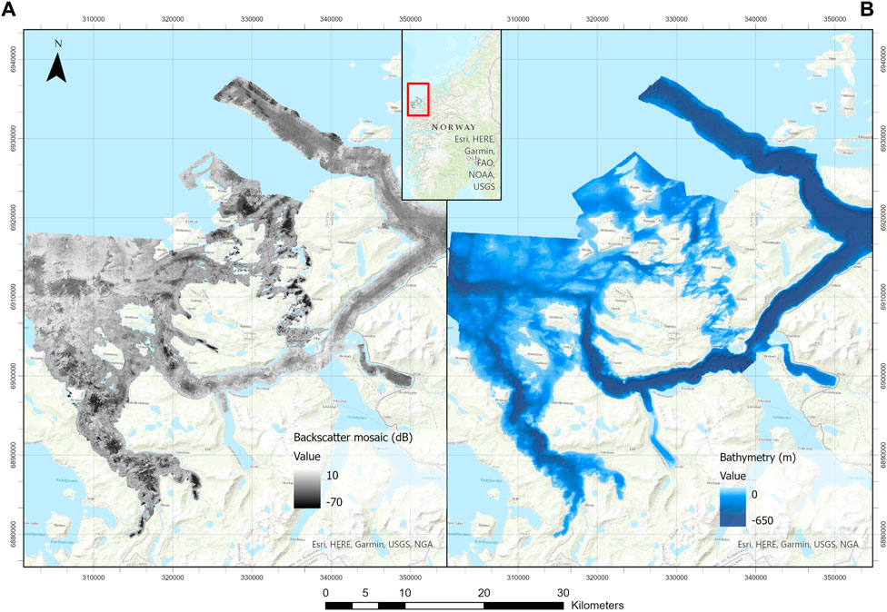
Figure 1. Overview of the study site and experimental data in the Søre Sunnmøre region of Norway. (A) MBES backscatter mosaic, (B) MBES bathymetry grid.

The MBES data was collected over 38 surveys taking place between 2006 and 2012 using four different MBES systems (Kongsberg Maritime models EM 710, EM1002, EM 3000 and EM 3002D), which covered a depth range of 0–636 m (Elvenes et al., 2019). The acoustic data were processed and gridded into a single digital bathymetry model (DBM) and a single backscatter mosaic, both of 1 m x 1 m horizontal resolution. A seabed sediment-type map of 25 classes was generated by a marine geology expert using manual digitization. The interpretation was based on the bathymetry grid (with overlaid hillshade), a slope raster (derived from the bathymetry grid), the backscatter mosaic, and shapefiles representing the classified sediment samples and towed video footage acquired over the area (Elvenes et al., 2019).

2.2 Data pre-processing

Since the marine geology expert also used the hillshade and slope for their interpretation, we also included these bathymetry derivatives to quantify their relevance. Slope and hillshade are related variables that emphasize the local morphology, while bathymetry display only allows visualizing the general depth trend. Slope is the measure (in degree units) of the maximum steepness for each cell of the bathymetry raster relative to its neighbour cells, while hillshade is a grayscale 3D representation of the morphology resulting from the simulation of a light source located at a given azimuth and direction relative to the site. We derived these two layers from the bathymetry grid using the “Slope”³ and “Hillshade”⁴ tools available in ArcGIS Pro (Figure 2). We utilized the “Hillshade” tool in ArcGIS Pro with its default parameters, configuring the “azimuth” to 315° from the northwest and “the altitude” to 45° above the horizon. The backscatter mosaic, the bathymetry, hillshade and slope layers were normalized to the 0–1 range and used as input features to the U-Net (Figure 3). The original 25-classes seabed map was simplified into “bedrock” and “non-bedrock” as described in Table 1 (Figure 4). This modified reference map was used as the U-Net’s target variable.

Figure 2

Figure 2. Illustration of the input features in our dateset: (A) Bathymetry grid (m) shown over the hillshade layer to highligth seabed topography, (B) Backscatter mosaic (dB), (C) Slope layer, (D) Hillshade layer.

Figure 3

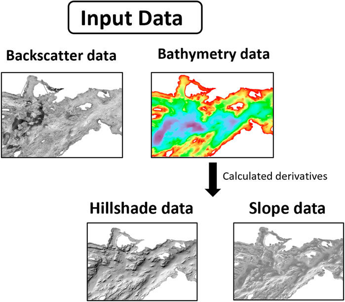
Figure 3. Input data layers: backscatter mosaic, bathymetry grid, and the hillshade and slope layers derived from the bathymetry grid.

Table 1

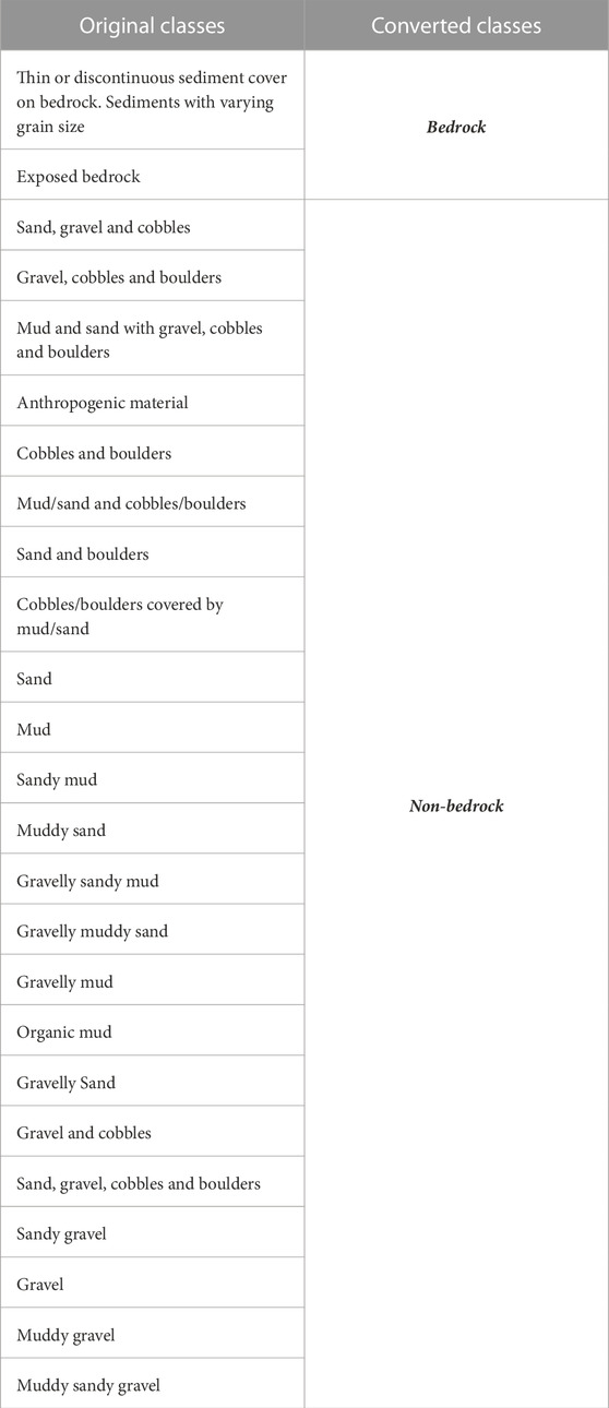
Table 1. Sediment classes conversion from the original NGU map for DL network training purposes.

Figure 4

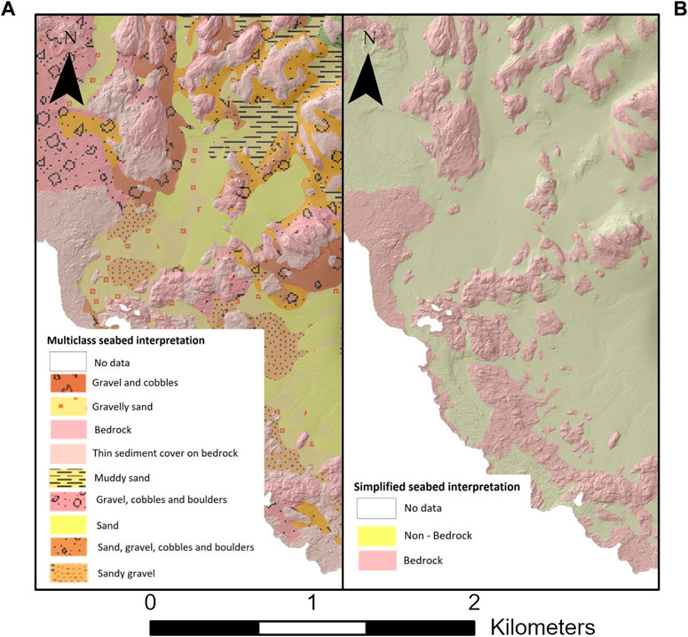
Figure 4. Extract of the original 25-classes seafloor sediment map, and the simplified binary bedrock/non-bedrock map. (A) Original multi-class sediment map, (B) Simplified sediment map.

For the generation of the training, validation and test datasets, we sampled the entire source dataset ensuring to spatially cover as much data as possible while also reducing the amount of no-data locations. This process resulted in 24 manually generated rectangular regions of variable dimensions (Figure 5). The regions without rectangles indicate locations where either some of the input data was missing, the expert map was unavailable, or the quality of the input data was inadequate. Figure 6A shows an area omitted from training due to local lack of data in the backscatter mosaic. Artifacts appeared frequently in our backscatter data, and although efforts were made to remove them from the training and validation dataset, a few still remained within the rectangular regions. Examples of typical artifacts characterizing our data are visible in Figures 6B, C.

Figure 5

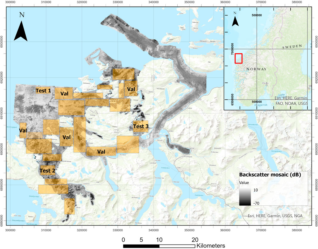
Figure 5. Location of the sampling rectangles over the study area overlaid on the backscatter mosaic. Rectangles labeled with “Test” were used as testing rectangles, rectangles labeled as “Val” were used as validation rectangles.

Figure 6

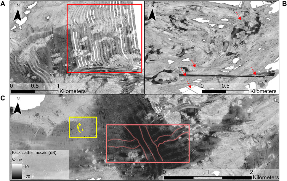
Figure 6. Examples of artifacts in the backscatter mosaic. (A) In the red rectangle is displayed an area of the mosaic excluded from training due to local lack of data, (B) Example of backscatter artifacts indicated by the red arrows, (C) The yellow frame include linear artifacts visible across the backscatter data, the orange frame shows the result of merging backscatter data acquired along different directions.

Each of the 24 rectangles was allocated either for training, validation or testing, with the split realized to ensure that the class frequencies across the three subsets were comparable and representative of the entire dataset (Figure 7). Across all subsets, the bedrock and the non-bedrock classes made up respectively 20%–25% and 55%–60% of all pixels, while the rest of the pixels belonged to the no-data/background class, which was used as a third class in models training but excluded from the network’s inferring and evaluation.

Figure 7

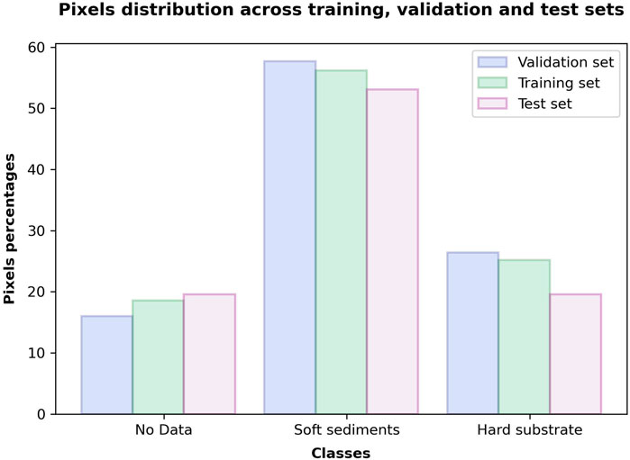
Figure 7. Class frequencies for the training, validation and test subsets.

To avoid artificially-improved classification performance, poor model generalization, and biased predictions due to spatial autocorrelation (Roberts et al., 2017; Schratz et al., 2019; Karasiak et al., 2022), we calculated the covariance function for both our testing and training data using ArcGIS Pro. By measuring the strength of statistical correlation as a function of distance, the covariance function quantifies the concept that close objects are more similar compared to those at greater distances⁵. Hence, by evaluating the covariance function we ensured a 1,000 m buffer distance between the training and the testing rectangles. This distance was selected according to the point at which the covariance function approached a value of 0 for all our data.

2.3 Models training, inferring and evaluation

Once the study area was sampled by extracting rectangles of data (bathymetry, backscatter, hillshade and slope), each rectangle was further divided into patches of 256 m x 256 m, with a 50% overlap between consecutive patches both along the X-axis and Y-axis. This resulted in approximately 22,000 patches of each MBES data type for training. We used the modified light-weight U-Net network described in Leclerc et al. (2019). U-Net is a convolutional neural network architecture known for its U-shaped architecture that combines contracting and expanding pathways by the mean of skip connections, the key component of the network aimed to merge encoder and decoder features (Ronneberger et al., 2015). The encoder consists of a contracting patch compressing the input data for feature extraction. The decoder involves an expanding path which uses upsampling and convolutional layers that, by recovering spatial details potentially lost during the downsampling, generate the segmented output map (Ronneberger et al., 2015; Leclerc et al., 2019).

We trained four models using a single data source in input (single-input models): either backscatter (M_B), depth (M_D), slope (M_S), or hillshade (M_H), and six models using two data sources (multiple-input models): backscatter and depth (M_BD), backscatter and hillshade (M_BH), backscatter and slope (M_BS), depth and slope (M_DS), depth and hillshade (M_DH), and slope and hillshade (M_SH) (Figure 8).

Figure 8

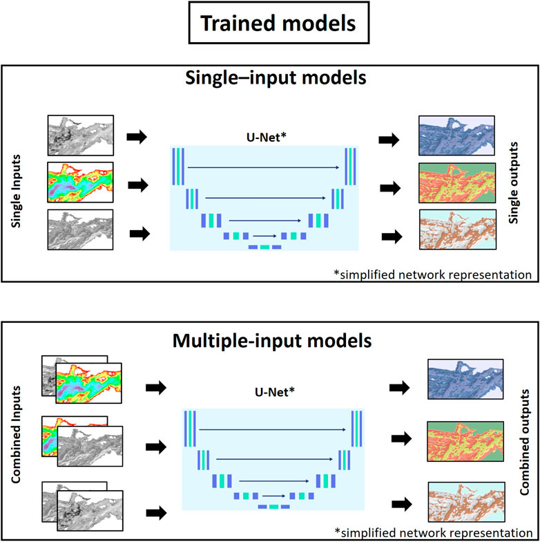
Figure 8. Summary of the U-Net models generated. Single feature models are models trained using single inputs (e.g., backscatter data, or slope data, or bathymetry data, etc.). Two-layers models were generated by inputting the network with two layers at the same time (e.g., backscatter + slope data, or depth data + hillshade data, etc.).

The trained models were used to infer predictions on the 50% overlapping consecutive 256 m x 256 m patches produced from the testing rectangles. In order to obtain a cohesive and smooth prediction for any given testing rectangle, the prediction patches were merged back together using an algorithm⁶ that blends overlapping data with a window function. This function assigns different weights to the pixels according to their position within each overlapping patch (pixels at the edge of a patch are given less weight than the pixels located at the centre of a patch).

The generalization performance of the trained models was evaluated by calculating the Dice Score (DS) coefficient (Milletari et al., 2016), the overall accuracy (Acc), the Kappa coefficient (Kappa) and the user’s and the producer’s accuracy for each class (class UAcc and PAcc) (Congalton, 1991). All these metrics, derived from the models’ confusion matrices and available as Supplemental Material, were calculated on the testing dataset for the predicted classes bedrock/non-bedrock and excluding the no-data class. The DS, is the most commonly used performance metric for semantic segmentation using Deep Learning (Bertels et al., 2019), the remaining metrics were added to encompass global and class-specific accuracy measurements, as suggested by Strahler et al. (2006). These represent the most common metrics used in the seabed classification literature (Li et al., 2016; Siwabessy et al., 2018; Turner et al., 2018), specifically, Liu et al. (2007) emphasize the importance of UAcc, PAcc and Acc as primary accuracy measures. The DS, Acc and Kappa are global metrics. The DS is a quantity ranging between 0 and 1 which measures the overlap among the models’ predictions and the reference annotations. The Acc metric is the ratio between the number of pixels correctly classified and the total number of classified pixels (Devaram et al., 2019). The kappa metric quantifies the level of agreement between two sets of categorical data by taking into account the agreement that could arise by chance, beyond what would be expected due to random concordance (Congalton, 1991; Warrens, 2015). PAcc and UAcc are both class-specific metrics, the first provides a measure of the pixels correctly classified in a particular category, as a percentage of the total number of pixels actually belonging to that category, the second informs that for all the areas classified as a certain category, a certain percentage are actually correct (Congalton, 1991).

In a post-processing stage, we also tested various values for the “decision threshold” parameter. Deep learning trained models provide the user with a measure of the certainty or uncertainty of the predictions in term of probabilities and sometimes the default threshold parameter (0.5) might be not optimal to represent correctly the distribution of the segmented classes of interest and the model might commit an error of misclassification towards certain classes (Fernández et al., 2018).

Finally, to gain insight in the sources of discrepancies between the model predictions and the reference map in the testing dataset, we calculated the percentage of pixels predicted as bedrock. This analysis was conducted to evaluate the accuracy of the predictions in relation to the original sediment classifications outlined in the reference map.

3 Results

Based on their inference on the test set, the models scored DS values ranging in 0.69–0.80 and Acc values ranging in 0.77–0.85 (Table 2). Among the single-input models, M_D and M_S consistently displayed the highest values for the majority of the metrics, while M_B exhibited the lowest performance. The results for the multiple-input models confirmed the higher predictive power of the depth and slope over backscatter, as all the multiple-input models incorporating backscatter data (M _BD, M _BH and M _BS) consistently showed lower performance metrics than the corresponding single-input models without backscatter data (respectively, M _D, M _H, and M _S). Noticeably, no multiple-input models outperformed the best single-input models.

Table 2

Table 2. Overview of the metrics calculated for both the single-layer and two-layers models.

Figure 9 illustrates the differences between the expert annotations and the predictions of the models which consistently scored high metrics (M_D and M_S) or low metrics values (M_B, M_BD), over a portion of the test set representative of topographically complex areas in our dataset. Overall, Figures 9B–E demonstrates that predictions from M_D and M_S more closely resemble the human interpretations, while M_B and M_BD deviates more. Furthermore, models trained using inputs from the same data source resulted in similar predictions (e.g.,.M_D and M_S or M_B and M_BD). This can be observed in Figure 10 where predictions from M_D and M_S are compared and almost perfectly overlap both for the bedrock class (Figure 10A) and for the non-bedrock class (Figure 10B). This figure shows that predictions from M_D and M_S overlap in almost every region of the seabed. Only a few differences between the models occur, and these are highlighted by the green areas, corresponding to pixels predicted as bedrock by the M_D model and by the orange areas, corresponding to pixels predicted as bedrock by the M_S model.

Figure 9

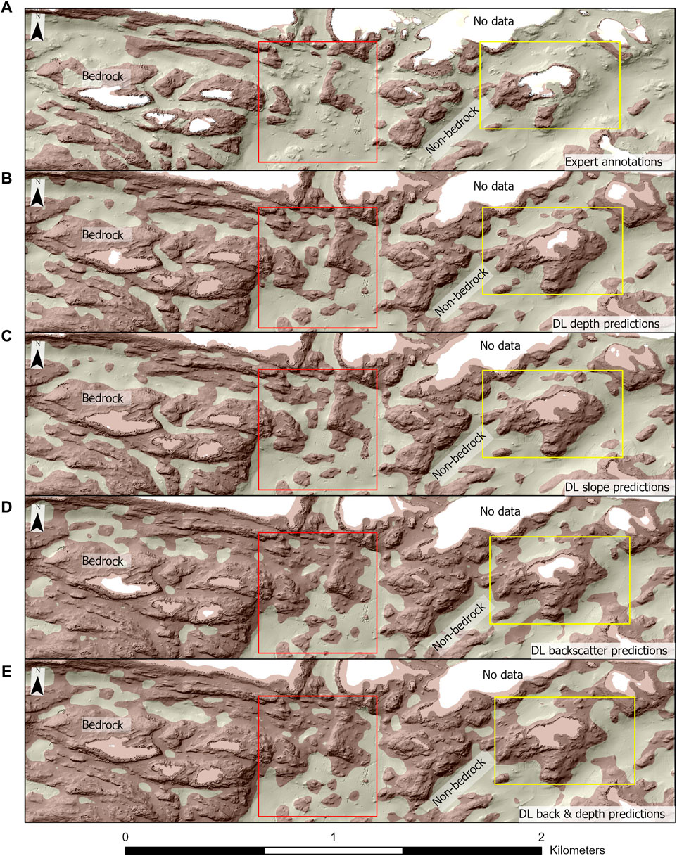
Figure 9. Comparison among the DL outputs and the original expert annotation. The area chosen to visualize the predictions belongs to one of the test rectangles used as test dataset. Red and yellow rectangles highlight areas of interest (see text). To better enhance the underling topography, predictions/annotations are shown over the hillshade layer. (A) Expert annotations, (B) M_B predictions, (C) M_D predictions, (D) M_S predictions, (E) M_BD predictions.

Figure 10

Figure 10. Comparison among the best performing DL outputs: the depth and the slope models. Both predictions are superimposed on the hillshade layer, which was selected for its ability to accentuate the topography. The area chosen to visualize the predictions belongs to one of the test rectangles used as test dataset. (A) The figure shows the slope and depth models’ predictions for the bedrock class. Here the background class encompasses the no-data and the non-bedrock areas. (B) The figure shows the slope and depth models’ predictions for the non-bedrock class. Here the background class encompasses the no-data and the bedrock areas.

An in-depth comparison of the maps in Figures 9B–E shows that all models tend to predict any seafloor area showing a complex bathymetric relief as bedrock, whether or not it was annotated as such by the expert. This observation is confirmed by the results listed in Table 2 where the PAcc values for the bedrock class for all the models are higher than the corresponding UAcc ones. This indicates an over-prediction of the bedrock class compared to the expert’s interpretation. Moreover, Figures 9B–E shows that both M_B and M_BD appear to have a more pronounced tendency to predict the bedrock class in flat areas compared to M_D and M_S.

While the models generally over-predict the bedrock class, as seen from the higher PAcc values compared to the corresponding UAcc values (Table 2) and from Figure 9, instances of underprediction are also evident. In Figure 11, model M_D, taken here as an example, fails to recognize expert-annotated bedrock regions in flat seabed areas. The tendency of locally failing to predict the bedrock class in flat seafloor areas, compared to the expert annotations, is a trend observed not just in M_D, but across all models.

Figure 11

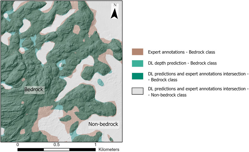
Figure 11. Example of under-prediction of the bedrock class for the model M_D. The predictions from the DL model M_D, are overlaid onto the expert annotations for a selected test rectangle. This illustration emphasizes the discrepancy between the expert annotations and the model predictions. While the expert includes flat areas of the seabed in their definition of bedrock, the DL model predominantly identifies bedrock in regions of the seafloor characterized by rough topographic features.

To gain insight into the relationship between the DL bedrock predictions and the original expert-annotated sediment classes within the testing rectangles, we conducted an analysis focusing on quantifying the degree of over-prediction for the bedrock class. The over-prediction, expressed as percentage, was calculated by dividing the number of pixels of each original class predicted as bedrock, by the total number of pixels predicted as bedrock. The findings are summarized in Table 3, which includes results from the models that consistently achieved high metrics or low metric values (M_D and M_S), M_B, and M_BD, and whose predictions were visualized in Figure 9. This table presents the original expert-annotated sediment classes, their corresponding converted classes used for the DL network training, and a column that shows the percentage of pixels for each of the original expert-annotated sediment classes in the testing dataset. In addition, for each considered model, we included a column showing the percentage of pixels from the original classes that were predicted as bedrock, out of the total number of pixels predicted as bedrock. As an example of the table interpretation, for the original class “exposed bedrock” and for the model M_D, 19.95% of the totality of pixels predicted as bedrock, corresponds to the original class “exposed bedrock”. The largest group of pixels misclassified as bedrock occurs for the original class “Sand, gravel, cobbles and boulders”, which is also the non-bedrock class most frequently mapped by the expert (11.66% of all pixels). Other pixels misclassified as bedrock belong to the classes “Sand, gravel, and cobbles” for M_D, M_S, and M_BD (over 3.68% of pixels misclassified as bedrock) and “Cobbles and boulders” for M_BD (2.82% of pixels misclassified as bedrock). These two classes are also among the most frequent non-bedrock classes in the expert map (respectively 6.76% and 6.66% of all pixels in the testing rectangles). While pixels from finer-grained sediment classes are also predicted as bedrock across the considered models, the percentage of such misclassified pixels is relatively lower. For instance, “Sandy mud” (the second most frequent non-bedrock class constituting 8.90% of all pixels) accounts for the 0.72%–0.78% of pixels predicted as bedrock by models M_D, M_S, and M_BD, and the 0.98% of pixels predicted as bedrock by model M_B.

Table 3

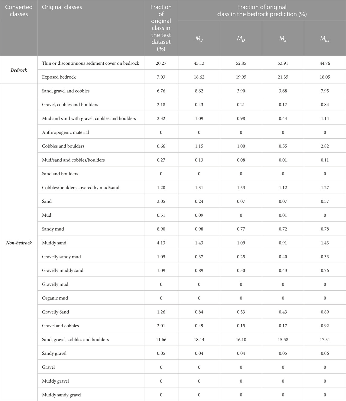
Table 3. The table analyzes the over-prediction of the bedrock class resulting in pixels predicted as bedrock even if belonging to a different original sediment class. The over-prediction of the bedrock was quantified by dividing the number of pixels of each original class predicted as bedrock, by the total number of pixels predicted as bedrock. These results are displayed respectively for the backscatter, depth, slope and the backscatter and depth models in the column “Fraction of original class in the bedrock prediction (%)”. A column showing the fraction of original sediment classes in the test dataset (%) has also been added. To be noted that the sum of percentages in this column adds up to 80.37%, the remaining 19.63% belongs the background class, not included in the calculation.

In an effort to mitigate the bedrock over-prediction, we tried increasing the ‘decision threshold’ parameter from its default value of 0.5. Threshold values between 0.7 and 0.8 yielded predictions similar to the default threshold. Threshold value of 0.9 marginally improved bedrock delineation in specific areas. Since we did not observe any consistent improvement with higher threshold values, we decided to use the default one of 0.5.

4 Discussion

The analysis conducted on the trained models reveals valuable insights about the DL models’ ability to classify the bedrock/non-bedrock classes from MBES data. The backscatter model shows the lowest performance metrics compared to the rest of the trained models. Conversely, all the models trained with bathymetry/bathymetry-derived data demonstrate consistently high comparable metrics. The visual assessment of the models’ predictions aligns with these findings. Predictions from M_D and M_S tend to follow the rough bathymetric relief more closely than M_B and M_BD. This is evident from the clear boundaries and sharp edges observed in the topographically rough areas mapped as bedrock (red and yellow rectangles in Figures 9C, D). In contrast, predictions from M_B and M_BD (Figure 9B, E) often lacked precision in delineating with detail bedrock areas that often appeared clustered together. The superior performance of models trained using bathymetry data can be attributed to their ability to recognize the locally complex morphology of the seabed as a distinctive feature of bedrock areas. This mirrors the practice of marine geology experts, who mainly rely on bathymetry data when delineating bedrock outcrops, while they use backscatter data primarily for distinguishing between several finer grained-sediment types (Elvenes et al., 2019). A likely factor contributing to the lower performance of backscatter models compared to bathymetry models, is the heterogeneous nature of the MBES data in our study, since it was collected across 38 surveys using 4 different MBES systems. In this heterogeneous dataset, different acquisition and processing parameters may have been applied, introducing misfits when generating a composite backscatter mosaic (Figure 6). These artifacts might have affected the recognizability of relevant backscatter acoustic patterns, making it difficult for the network to reliably predict the classes of interest. An attempt to re-process the available data might help unveil whether the low performances can be mainly attributed to the nature of the data. Another possible reason for the weak performance of the models using backscatter is that the backscatter strength from bedrock may vary considerable, due to variations in roughness both on micro and macro scale. Furthermore, MBES systems with different frequencies may respond differently. The MBES system EM710 uses frequencies between 70 and 100 kHz, while the EM 3000 and EM3002D systems use frequencies in the 300 kHz band. These findings strongly indicate that for this particular experiment, backscatter data might have limited relevance, compared to the bathymetry data, for effectively classifying bedrock/non-bedrock classes.

Our results also showed that the combination of two data sources for training did not enhance the seabed classification quality compared to the use of any single data source. In general, combining different data sources is expected to enhance deep learning models’ predictive capability by capturing complementary information and patterns within the data. However, we found that multiple-input models using depth and depth derived data (M_DH, M_DS, M_SH) did not achieve a higher performance than the single-input models (Table 2). All these models share the common characteristics of learning features from the same data source, namely, the bathymetry. It can be thus inferred that U-Net can effectively generate all the necessary data representations from the bathymetry data alone. These findings differ from those presented in the study conducted by (Arosio et al., 2023) where a combination of bathymetry and hillshade data sources yielded DL models with the best performance. This difference in results may stem from the specific classification tasks of each study, in fact while Arosio et al. (2023) aimed to identify various seabed morphological classes, including distinct rock textures, we focused solely on bedrock/non-bedrock separation. Furthermore, our study utilized a high-resolution, expert-generated map for annotation, in contrast to the limited annotated data employed by Arosio et al. (2023). Although the disparities in our classification objectives and available data may account for our differing results, further research is essential to fully unravel the underlying causes of these discrepancies.

Despite the different nature of the backscatter and depth/depth derivatives data, the combination of these data sources did not improve our DL models’ performance either. M_BD, M_BH and M_BS showed a varied range of performance, but it was in each case lower compared to the corresponding single-layer model without the backscatter layer (Table 2). Apart from the already discussed backscatter data limitations, the observed performance degradation may indicate that the available data might not be sufficient for effectively training the combined-layers models. Further research aimed to test the use of augmentation techniques to artificially increase the size of the training data, might enable the models to learn more efficiently the backscatter acoustic patterns that characterise bedrock/non-bedrock and improve their generalization performance.

The over-prediction of the bedrock class plays an important role in our experiment as it results in pixels predicted as bedrock even if belonging to a different original sediment class. For all the models, the largest group of pixels misclassified as bedrock occurs for the original classes “Sand, gravel, cobbles and boulders”, “Sand, gravel, and cobbles”, and “Cobbles and boulders” (Table 3). For these classes, the seabed surface characteristics from bathymetry data may resemble those of bedrock, making it difficult for the network to differentiate between these sediments and the bedrock classes. Similarly, the backscatter response of these sediments can, under specific circumstances, show similarities to the backscatter response of bedrock. One such scenario might occur when the “Sand, gravel, and cobbles” class is found in close proximity to bedrock outcrops, resulting in a highly complex seabed surface. The presence of transitional features in the backscatter data can lead to ambiguous acoustic patterns that can be challenging to distinguish. Hence, this can lead to errors of misclassifications or less accurate predictions for both the “Sand, gravel, and cobbles” class and bedrock class in such areas. Finally, it can be observed that pixels belonging to finer grained sediments fractions are also misclassified as bedrock. Factors contributing to pixels’ misclassifications for these classes might include variability within the sediment classes (making it difficult for the network to differentiate among similar classes), quality of the training samples, and potential limitations in data resolution. The latter, in particular, can affect the ability of the models to capture subtle differences between sediment types. Overall, despite the error in overpredicting the bedrock class, when occurring for well-performing models such as M_D and M_S, the over-prediction could provide valuable insights for advancing research in seabed classification using deep learning. Indeed, areas where over-prediction occurs could be considered indicators of geologically heterogeneous/complex areas of the seabed that necessitate further investigations to gain a deeper understanding of the factors contributing to the models’ errors.

While the over-prediction of bedrock is a significant factor, it is important to note that under-prediction of the bedrock class also plays a crucial role in our experiment. We observed instances where the expert-annotated bedrock extended beyond areas characterized by topographic roughness, as shown in Figure 11. Conversely, the DL network predominantly predicted bedrock in seabed areas with distinct rough topographic features. While it may be challenging to definitively determine whether the DL model or the annotator’s interpretation is correct for the areas in which under-prediction occurs, several factors such as the scale at which the interpretation is performed and the subjective nature of manual mapping could contribute to the differences between expert annotations and DL predictions. To address these disparities, for example, collaborative efforts involving expert geologists in establishing annotation guidelines for sediment classes, including bedrock, could lead to the creation of standardized criteria for identifying bedrock, potentially improving the accuracy of DL predictions.

The decision threshold experiment, aimed to minimize the bedrock’s over-prediction, showed no consistently improved performance metrics over the test set. Future research might reveal if the manual tuning of this parameter could be a valuable technique for expert users that could leverage their interpretative skills and understanding of the data to arbitrarily match predictions with the seabed topography when desired. This prospect of combining DL predictions and human input, as the research in this field progresses, could enable a faster and more efficient approach to seabed sediment mapping than simply relying on either one.

Overall, the misclassification error should also be analysed by considering the inherent nature of manual and automatic methods for seabed mapping. When manually generating maps of the seabed, the experts leverage their experience of sediment characteristics for identifying and extracting relevant seabed features to be used for seabed classification (Diesing et al., 2014; Janiesch et al., 2021). Therefore, experts generated maps provide us with a wide comprehension of the spatial distribution of sediments and the best representation of the seabed sediments distribution. This stands in contrast to situations where sediments information is only limited to sparse ground-truth locations, resulting in an incomplete representation of the sediment distribution across the seabed. However, different experts may interpret the data in different ways and factors such as sparse ground-truth samples locations might affect the quality of the interpreted map. As a consequence, the process of manual mapping unavoidably introduces a certain level of uncertainty. In comparison, DL algorithms, if trained with sufficient amount of data and reliable annotations, can automatically learn relevant seabed features from the data. This reduces subjectivity in feature engineering and can yield predictions that are potentially more reliable and consistent than those generated by humans.

As briefly introduced when discussing the under-prediction of the bedrock class, the scale of interpretation at which the mapping is conducted, is another factor posing a challenge for the DL models. During the manual generation of seabed sediments maps, expert geologists can contextualize any pixel using its neighboring region, at any desirable scale. In comparison, our models operated on a fixed scale, 256 m x 256 m patches of data, which limits the geological and geographical context of the pixels. Further investigations aimed to explore the limitations of the geographical scale and methods to incorporate information among overlapping patches would contribute to improving the reliability and performance of our models. In addition, the scale also contributes to the misclassification error. The reference map was generated at a 1:20,000 scale (Elvenes et al., 2019). Consequently, given the MBES data resolution of 1 m x 1 m, the DL models could have generated predictions with a higher level of detail compared to the reference map. As a result, the mismatch between the predictions and the ground truth led to a misclassification error.

Finally, it is important to consider that our DL models were both trained and assessed using a manually delineated map as the ground-truth. However, using experts’ generated maps as a reference for training, even though they provide the most accurate representation of seabed sediments, introduces the risk of inheriting limitations and biases present in the manual interpretation process. As a consequence, the quality of the models’ predictions might be affected. All the metrics were evaluated based on the comparison between the DL and the human generated maps disregarding any potential sources of error or subjectivity that could be inherent to the latter. This is also true for the visual assessment of our DL predictions. In summary, we used an evaluation approach that focused on assessing how closely our DL models resembled the expert-generated map, rather than directly measuring the models accuracy in predicting seafloor types.

We currently cannot assess whether our models outperform human interpreters and whether the predicted maps are more accurate than the manually annotated ones. In fact, while we can evaluate the goodness of our predictions by comparing them to the human-generated map, this method leaves us with uncertainties regarding the objective performance of our models. To gain a more comprehensive understanding of their accuracy in predicting seafloor types, further investigations are necessary. Further evaluations comparing predictions against additional ground-truth data or maps produced by other experts could be conducted. Additionally, seeking opinions from third-party expert evaluators could provide valuable insights and support in discerning the potential strengths and limitations of both our approach and human interpretation. Such efforts would contribute to a more robust assessment of our models’ performance and their capabilities in predicting seafloor types accurately.

Utilizing a human-generated map as the ground truth for training deep learning models represents a novel approach. To our knowledge, this technique has solely been tested in remote-sensing applications to map the bedrock in onshore areas (Ganerød et al., 2023). Therefore, we could not directly compare the outcome of our research to other studies. Nevertheless, the promising results achieved through this technique underscore its potential to provide a novel perspective for conducting seabed classification in both onshore and offshore settings.

4.1 Final remarks and future directions

This study evaluated the potential of the Deep Learning network U-Net in classifying the seabed sediments into either bedrock and non-bedrock, using MBES bathymetry and backscatter data. Deep learning models showed great promise in seabed sediments classification. Results showed that the models utilizing bathymetry and bathymetry-derived data achieved better separation of the classes and were able to reliably generate predicted seabed sediment maps comparable to a manually-generated seabed map. Noticeably, all the generated models showed the tendency to overpredict the bedrock class. As they were all trained and evaluated using a manually generated map, it could not be determined whether the models yielded more accurate predictions of the seafloor sediments than the expert ones. Further work should include an inter-observer analysis to shed light on the level of subjectiveness of an expert map, and to evaluate the maps produced by the models against the ground-truth (e.g., video footage). Until then, the models with the highest accuracy could represent a valuable aid to the human experts who could use the predicted maps and modify them according to their discretion and expertise.

Although a widely-accepted standard of automatic method for seabed classification has not been established yet, the findings in this paper offer assistance in expediting the process. In future research, it would be valuable to produce models trained over more than the two classes used in the current study. In addition, as a requirement for establishing a model for actual use, it would be necessary to test the best-performing models on a new, independent set of MBES data, acquired in a distinct geographical area, yet characterized by similar geological properties. A positive outcome from these analyses would help to understand if U-Net models have the ability to leverage the acquired knowledge to predict comparable datasets with limited or no re-training. This finding has the potential to be a significant advancement that could also make the way for real-time mapping applications.

Data availability statement

The datasets presented in this article are not readily available because raw MBES data were provided by NGU. Seabed sediment maps of the studied area are free to access to and can be found at www.mareano.no and www.ngu.no. Requests to access the datasets should be directed to TT, Senior Marine Geologist at NGU (terje.thorsnes@ngu.no).

Author contributions

RG: Conceptualization, Data curation, Investigation, Methodology, Project administration, Software, Visualization, Writing–original draft, Writing–review and editing. TB: Conceptualization, Methodology, Supervision, Validation, Writing–review and editing. AS: Conceptualization, Methodology, Supervision, Validation, Writing–review and editing. MD: Supervision, Validation, Writing–review and editing. TT: Supervision, Validation, Writing–review and editing. LL: Conceptualization, Methodology, Supervision, Validation, Writing–review and editing.

Funding

The author(s) declare financial support was received for the research, authorship, and/or publication of this article. This study was funded by grants from the Centre for Innovative Ultrasound Solutions (CIUS) at Norwegian University of Science and Technology (NTNU). CIUS is a centre of excellence for research-based innovations supported by the Research Council of Norway, NTNU and industrial and clinical partners. The study was further supported by the NTNU industrial partner Kongsberg Discovery, and the Geological Survey of Norway (NGU) through the MAREANO programme (www.mareano.no).

Acknowledgments

We extend our appreciation to Sigrid Elvenes from the Geological Survey of Norway (Trondheim, Norway) and Frank Tichy from Kongsberg Discovery (Horten, Norway) for their valuable support and suggestions during the preparation of this paper.

Conflict of interest

The authors declare that the research was conducted in the absence of any commercial or financial relationships that could be construed as a potential conflict of interest.

Publisher’s note

All claims expressed in this article are solely those of the authors and do not necessarily represent those of their affiliated organizations, or those of the publisher, the editors and the reviewers. Any product that may be evaluated in this article, or claim that may be made by its manufacturer, is not guaranteed or endorsed by the publisher.

Supplementary material

The Supplementary Material for this article can be found online at: https://www.frontiersin.org/articles/10.3389/feart.2023.1285368/full#supplementary-material

Footnotes

¹https://www.ngu.no/.

²https://www.mareano.no/.

³https://pro.arcgis.com/en/pro-app/latest/tool-reference/spatial-analyst/slope.htm.

⁴https://pro.arcgis.com/en/pro-app/latest/help/analysis/raster-functions/hillshade-function.htm.

⁵https://pro.arcgis.com/en/pro-app/latest/help/analysis/geostatistical-analyst/semivariogram-and-covariance-functions.htm.

⁶https://github.com/Vooban/Smoothly-Blend-Image-Patches.

References

Anokye, M., Cui, X., Yang, F., Fan, M., Luo, Y., and Liu, H. (2023). CNN multibeam seabed sediment classification combined with a novel feature optimization method. Math. Geosci., 1–24. doi:10.1007/s11004-023-10079-5

CrossRef Full Text | Google Scholar

Arosio, R., Hobley, B., Wheeler, A. J., Sacchetti, F., Conti, L. A., Furey, T., et al. (2023). Fully convolutional neural networks applied to large-scale marine morphology mapping. Front. Mar. Sci. 10. doi:10.3389/fmars.2023.1228867

CrossRef Full Text | Google Scholar

Bertels, J., Eelbode, T., Berman, M., Vandermeulen, D., Maes, F., Bisschops, R., et al. (2019). “Optimizing the dice score and jaccard index for medical image segmentation: theory and practice,” in Medical Image Computing and Computer Assisted Intervention–MICCAI 2019: 22nd International Conference, Shenzhen, China, October 13–17, 92–100.

CrossRef Full Text | Google Scholar

Brown, C. J., and Collier, J. S. (2008). Mapping benthic habitat in regions of gradational substrata: an automated approach utilising geophysical, geological, and biological relationships. Estuar. Coast. Shelf Sci. 78, 203–214. doi:10.1016/j.ecss.2007.11.026

CrossRef Full Text | Google Scholar

Brown, C. J., Sameoto, J. A., and Smith, S. J. (2012). Multiple methods, maps, and management applications: purpose made seafloor maps in support of ocean management. J. Sea Res. 72, 1–13. doi:10.1016/j.seares.2012.04.009

CrossRef Full Text | Google Scholar

Brown, C. J., Smith, S. J., Lawton, P., and Anderson, J. T. (2011). Benthic habitat mapping: a review of progress towards improved understanding of the spatial ecology of the seafloor using acoustic techniques. Estuar. Coast. Shelf Sci. 92, 502–520. doi:10.1016/j.ecss.2011.02.007

CrossRef Full Text | Google Scholar

Buhl-Mortensen, L., Buhl-Mortensen, P., Dolan, M. F., and Holte, B. (2015). The MAREANO programme–a full coverage mapping of the Norwegian off-shore benthic environment and fauna. Mar. Biol. Res. 11, 4–17. doi:10.1080/17451000.2014.952312

CrossRef Full Text | Google Scholar

Congalton, R. G. (1991). A review of assessing the accuracy of classifications of remotely sensed data. Remote Sens. Environ. 37, 35–46. doi:10.1016/0034-4257(91)90048-b

CrossRef Full Text | Google Scholar

Cui, X., Yang, F., Wang, X., Ai, B., Luo, Y., and Ma, D. (2021). Deep learning model for seabed sediment classification based on fuzzy ranking feature optimization. Mar. Geol. 432, 106390. doi:10.1016/j.margeo.2020.106390

CrossRef Full Text | Google Scholar

Devaram, R. R., Allegra, D., Gallo, G., and Stanco, F. (2019). “Hyperspectral image classification via convolutional neural network based on dilation layers,” in Image Analysis and Processing–ICIAP 2019: 20th International Conference, Trento, Italy, September 9–13, 2019, 378–387.

CrossRef Full Text | Google Scholar

Diesing, M., Green, S. L., Stephens, D., Lark, R. M., Stewart, H. A., and Dove, D. (2014). Mapping seabed sediments: comparison of manual, geostatistical, object-based image analysis and machine learning approaches. Cont. Shelf Res. 84, 107–119. doi:10.1016/j.csr.2014.05.004

CrossRef Full Text | Google Scholar

Diesing, M., Mitchell, P. J., O’Keeffe, E., Gavazzi, G. O., and Bas, T. L. (2020). Limitations of predicting substrate classes on a sedimentary complex but morphologically simple seabed. Remote Sens. 12, 3398. doi:10.3390/rs12203398

CrossRef Full Text | Google Scholar

Elvenes, S., Bøe, R., Lepland, A., and Dolan, M. (2019). Seabed sediments of Søre Sunnmøre, Norway. J. Maps 15, 686–696. doi:10.1080/17445647.2019.1659865

CrossRef Full Text | Google Scholar

Fernández, A., García, S., Galar, M., Prati, R. C., Krawczyk, B., and Herrera, F. (2018). Learning from imbalanced data sets. Berlin, Germany: Springer.

Google Scholar

Ganerød, A. J., Bakkestuen, V., Calovi, M., Fredin, O., and Rød, J. K. (2023). Where are the outcrops? automatic delineation of bedrock from sediments using deep-learning techniques. Appl. Comput. Geosciences 18, 100119. doi:10.1016/j.acags.2023.100119

CrossRef Full Text | Google Scholar

Harrison, D., De Leo, F. C., Gallin, W. J., Mir, F., Marini, S., and Leys, S. P. (2021). Machine learning applications of convolutional neural networks and U-Net architecture to predict and classify demosponge behavior. Water 13, 2512. doi:10.3390/w13182512

CrossRef Full Text | Google Scholar

Ierodiaconou, D., Monk, J., Rattray, A., Laurenson, L., and Versace, V. (2011). Comparison of automated classification techniques for predicting benthic biological communities using hydroacoustics and video observations. Cont. Shelf Res. 31, S28–S38. doi:10.1016/j.csr.2010.01.012

CrossRef Full Text | Google Scholar

Janiesch, C., Zschech, P., and Heinrich, K. (2021). Machine learning and deep learning. Electron. Mark. 31, 685–695. doi:10.1007/s12525-021-00475-2

CrossRef Full Text | Google Scholar

Karasiak, N., Dejoux, J.-F., Monteil, C., and Sheeren, D. (2022). Spatial dependence between training and test sets: another pitfall of classification accuracy assessment in remote sensing. Mach. Learn. 111, 2715–2740. doi:10.1007/s10994-021-05972-1

CrossRef Full Text | Google Scholar

Lateef, F., and Ruichek, Y. (2019). Survey on semantic segmentation using deep learning techniques. Neurocomputing 338, 321–348. doi:10.1016/j.neucom.2019.02.003

CrossRef Full Text | Google Scholar

Lathrop, R. G., Cole, M., Senyk, N., and Butman, B. (2006). Seafloor habitat mapping of the New York Bight incorporating sidescan sonar data. Estuar. Coast. Shelf Sci. 68, 221–230. doi:10.1016/j.ecss.2006.01.019

CrossRef Full Text | Google Scholar

Leclerc, S., Smistad, E., Pedrosa, J., Østvik, A., Cervenansky, F., Espinosa, F., et al. (2019). Deep learning for segmentation using an open large-scale dataset in 2d echocardiography. IEEE Trans. Med. imaging 38, 2198–2210. doi:10.1109/tmi.2019.2900516

PubMed Abstract | CrossRef Full Text | Google Scholar

Li, J., Tran, M., and Siwabessy, J. (2016). Selecting optimal random forest predictive models: a case study on predicting the spatial distribution of seabed hardness. PloS one 11, e0149089. doi:10.1371/journal.pone.0149089

PubMed Abstract | CrossRef Full Text | Google Scholar

Liu, C., Frazier, P., and Kumar, L. (2007). “Comparative assessment of the measures of thematic classification accuracy,” in Remote sensing of environment. Elsevier, 107 (4), 606–616.

CrossRef Full Text | Google Scholar

Mayer, L., Jakobsson, M., Allen, G., Dorschel, B., Falconer, R., Ferrini, V., et al. (2018). The nippon foundation—GEBCO seabed 2030 project: the quest to see the world’s oceans completely mapped by 2030. Geosciences 8, 63. doi:10.3390/geosciences8020063

CrossRef Full Text | Google Scholar

Milletari, F., Navab, N., and Ahmadi, S.-A. (2016). V-net: fully convolutional neural networks for volumetric medical image segmentation. 2016 fourth Int. Conf. 3D Vis. 3DV, 565–571.

CrossRef Full Text | Google Scholar

Nezla, N., Haridas, T. M., and Supriya, M. (2021). “Semantic segmentation of underwater images using unet architecture based deep convolutional encoder decoder model,” in 2021 7th International Conference on Advanced Computing and Communication Systems (ICACCS) (IEEE), Coimbatore, India, 19-20 March 2021, 28–33.

CrossRef Full Text | Google Scholar

Qin, X., Luo, X., Wu, Z., and Shang, J. (2021). Optimizing the sediment classification of small side-scan sonar images based on deep learning. IEEE Access 9, 29416–29428. doi:10.1109/access.2021.3052206

CrossRef Full Text | Google Scholar

Roberts, D. R., Bahn, V., Ciuti, S., Boyce, M. S., Elith, J., Guillera-Arroita, G., et al. (2017). Cross-validation strategies for data with temporal, spatial, hierarchical, or phylogenetic structure. Ecography 40, 913–929. doi:10.1111/ecog.02881

CrossRef Full Text | Google Scholar

Ronneberger, O., Fischer, P., and Brox, T. (2015). “U-net: Convolutional networks for biomedical image segmentation,” in International Conference on Medical image computing and computer-assisted intervention, Vancouver, BC, Canada, October 8–12, 2015, 234–241

CrossRef Full Text | Google Scholar

Schratz, P., Muenchow, J., Iturritxa, E., Richter, J., and Brenning, A. (2019). Hyperparameter tuning and performance assessment of statistical and machine-learning algorithms using spatial data. Ecol. Model. 406, 109–120. doi:10.1016/j.ecolmodel.2019.06.002

CrossRef Full Text | Google Scholar

Siwabessy, P. J. W., Tran, M., Picard, K., Brooke, B. P., Huang, Z., Smit, N., et al. (2018). Modelling the distribution of hard seabed using calibrated multibeam acoustic backscatter data in a tropical, macrotidal embayment: Darwin harbour, Australia. Mar. Geophys. Res. 39, 249–269. doi:10.1007/s11001-017-9314-7

CrossRef Full Text | Google Scholar

Stephens, D., and Diesing, M. (2014). A comparison of supervised classification methods for the prediction of substrate type using multibeam acoustic and legacy grain-size data. PloS one 9, e93950. doi:10.1371/journal.pone.0093950

PubMed Abstract | CrossRef Full Text | Google Scholar

Strahler, A. H., Boschetti, L., Foody, G. M., Friedl, M. A., Hansen, M. C., Herold, M., et al. (2006). Global land cover validation: recommendations for evaluation and accuracy assessment of global land cover maps. European Communities, Luxembourg.51 (4), 1–16.

Google Scholar

Turner, J. A., Babcock, R. C., Hovey, R., and Kendrick, G. A. (2018). Can single classifiers be as useful as model ensembles to produce benthic seabed substratum maps? Estuar. Coast. Shelf Sci. 204, 149–163. doi:10.1016/j.ecss.2018.02.028

CrossRef Full Text | Google Scholar

Wang, H., Dong, L., Song, W., Zhao, X., Xia, J., and Liu, T. (2022). Improved U-Net-based novel segmentation algorithm for underwater mineral image. Intelligent Automation Soft Comput. 32, 1573–1586. doi:10.32604/iasc.2022.023994

CrossRef Full Text | Google Scholar

Warrens, M. J. (2015). Five ways to look at cohen’s kappa. J. Psychol. Psychotherapy 5. doi:10.4172/2161-0487.1000197

CrossRef Full Text | Google Scholar

Wei, L., Kong, S., Wu, Y., and Yu, J. (2022). Image semantic segmentation of underwater garbage with modified u-net architecture model. Sensors 22, 6546. doi:10.3390/s22176546

PubMed Abstract | CrossRef Full Text | Google Scholar