Tropical cyclone intensity estimation through convolutional neural network transfer learning using two geostationary satellite datasets

Accurate prediction and monitoring of tropical cyclone (TC) intensity are crucial for saving lives, mitigating damages, and improving disaster response measures. In this study, we used a convolutional neural network (CNN) model to estimate TC intensity in the western North Pacific using Geo-KOMPSAT-2A (GK2A) satellite data. Given that the GK2A data cover only the period since 2019, we applied transfer learning to the model using information learned from previous Communication, Ocean, and Meteorological Satellite (COMS) data, which cover a considerably longer period (2011–2019). Transfer learning is a powerful technique that can improve the performance of a model even if the target task is based on a small amount of data. Experiments with various transfer learning methods using the GK2A and COMS data showed that the frozen–fine-tuning method had the best performance due to the high similarity between the two datasets. The test results for 2021 showed that employing transfer learning led to a 20% reduction in the root mean square error (RMSE) compared to models using only GK2A data. For the operational model, which additionally used TC images and intensities from 6 h earlier, transfer learning reduced the RMSE by 5.5%. These results suggest that transfer learning may represent a new breakthrough in geostationary satellite image–based TC intensity estimation, for which continuous long-term data are not always available.

1 Introduction

Tropical cyclones (TCs), some of the most powerful and destructive natural phenomena, result in a significant number of fatalities and have adverse social and economic effects. To minimize the damage that they cause, it is necessary to accurately analyze and predict their intensity (maximum sustained wind speed). Because obtaining observational data over the sea is arduous, satellite image data are important for estimating TC intensity. The fundamental concept behind using satellite images for this purpose is that TC intensity is closely related to the cloud patterns in the images (Chen et al., 2018; Lee et al., 2021; Kim et al., 2022). A widely used method for applying this idea is the Dvorak technique, which estimates TC intensity based on the manual recognition of cloud patterns observed in geostationary satellite infrared (IR) imagery (Dvorak, 1975; Dvorak, 1984). Several upgraded versions of this technique have been proposed, including the digital Dvorak method, the objective Dvorak technique (ODT), and the advanced ODT. These upgraded techniques have reduced the uncertainty and variability of TC intensity estimations compared to the traditional Dvorak technique (Tan et al., 2022).

One of the reasons for the success of the Dvorak technique is that IR brightness temperature can be used as an indicator of important structural properties of a TC. Since the development of the Dvorak technique, studies have estimated TC intensity using parameters calculated based on IR brightness temperature. For example, the deviation angle variance technique estimates TC intensity by quantifying TCs’ axisymmetry by calculating the slope of the IR brightness temperature (Pineros et al., 2008; Ritchie et al., 2014). Another study (Sanabia et al., 2014) estimated TC intensity by analyzing the radial profile of the IR brightness temperature. Other studies have used traditional machine learning for TC intensity estimations (Piñeros et al., 2011; Liu et al., 2015; Zhao et al., 2016).

A convolutional neural network (CNN), an artificial intelligence technique, is similar to the Dvorak technique in that it identifies key patterns in images. Many researchers have proposed models based on deep CNNs to estimate TC intensity and demonstrated that the feature maps of CNNs show the key patterns of TCs (the distinct eyes of TCs, central dense overcast, and upper curvature of TC structures) well (Pradhan et al., 2018; Chen and Yu, 2021; Wang et al., 2022). The data used to train such models are either single-channel (Chen et al., 2019b; Chen et al., 2020; Tian et al., 2020; Zhang et al., 2021) or multi-channel satellite images (Pradhan et al., 2018; Lee et al., 2019a; Jiang and Tao, 2022; Tan et al., 2022; Tian et al., 2022; Zhang et al., 2022). Lee et al. (2019a) showed that using multichannel images achieved better performance (by ∼35%) than using single-channel images. Recently, substantial research has been conducted to improve CNN algorithms. Tan et al. (2022) embedded both residual learning and attention mechanisms in a CNN model to optimize its structure and improve its feature extraction ability. Zhang et al. (2022) devised a spatiotemporal encoding module (called STE-TC) and DenseConvMixer to improve the estimation performance of CNN models.

Data generated by Korea’s first geostationary satellite, the Communication, Ocean, and Meteorological Satellite (COMS), has been used in various research (Baek and Choi, 2012; Cho and Suh, 2013; Choi et al., 2014; Baik and Choi, 2015; Lee et al., 2019b; Yeom et al., 2019), including studies on TC intensity and size (Kwon, 2012; Lee and Kwon, 2015; Lee et al., 2019a; Lee et al., 2020; Baek et al., 2022). COMS was launched in 2010 and provided data for about 9 years, from April 2011 to March 2020, consisting of one visible channel and four IR channels. Its successor, Geo-KOMPSAT-2A (GK2A), launched in December 2018, has been collecting data since July 2019. GK2A currently has about 4 years’ worth of data and consists of four visible channels, two near-IR channels, and 10 IR channels. Although GK2A has higher spatial and temporal resolution than COMS, the data that it has accumulated thus far are not adequate for estimating TC intensity using these data alone. Therefore, in this study, we employed transfer learning techniques to use both COMS and GK2A data.

Transfer learning is a machine learning technique in which a learning model developed for a first learning task is reused as the starting point for another learning model to perform a second task (Taherkhani et al., 2020). Due to the difficulty of achieving high accuracy in computer vision and other domains when using finite training datasets, deep learning models often require vast datasets (Cao et al., 2016; Gorban et al., 2020; Li et al., 2020). Transfer learning offers a viable solution to this issue by transferring knowledge from the source domain to the target domain and enhancing the accuracy of deep learning models (Pan et al., 2011; Yang et al., 2017; Liu et al., 2018; Jiang et al., 2019). Transfer learning techniques can be used to expedite training, improve generalization, and compensate for data shortages (Pan and Yang, 2010; Deo et al., 2017). Combinido et al. (2018) used CNN transfer learning to estimate TC intensity solely based on grayscale IR images of TCs. Using the Visual Geometry Group 19-layer (VGG19) model to estimate TC intensity, they found that retraining only the last convolutional layer on TC images yielded modest performance. Pang et al. (2021) proposed a new detection framework for TCs (NDFTC) based on meteorological satellite images by combining a deep convolutional generative adversarial network (DCGAN) and the You Only Look Once (YOLO) v3 model through deep transfer learning. Such a model achieved better stability and accuracy than the model without transfer learning. Transfer learning has also been used in the fields of agriculture, industry, medicine, and natural science, showing improved performance over models without it (Deepak and Ameer, 2019; Ham et al., 2019; Imoto et al., 2019; Rahman et al., 2020; Aslan et al., 2021; Hassan et al., 2021).

In this study, we applied various transfer learning techniques to four COMS and GK2A IR channels to identify the optimal technique for both datasets and investigate its TC intensity estimation performance. Since the technique to be chosen depends on the nature of the data used, we conducted sensitivity experiments on three techniques: frozen, fine-tuning, and frozen–fine-tuning. This is the first study to use transfer learning techniques to estimate TC intensity using the COMS and GK2A datasets. We applied the selected techniques to (i) a model that estimates TC intensity using only current satellite images and (ii) an operational model that aims to estimate TC intensity in real time using all available data, including satellite images and TC intensity information from 6 h earlier in addition to current satellite images. We developed the latter based on the fact that the Dvorak method and TC prediction centers use all available past TC information to predict the current TC intensity.

The rest of this paper is organized as follows. Section 2 provides information of the dataset. Section 3 describes the method. Section 4 discusses the results of the model. Section 5 presents a discussion and conclusion.

2 Data

2.1 Best-track data

In this study, we used the TC intensity provided by TC best tracks as label data. Since the model that we aimed to develop was intended to estimate TC intensity using best-track data from the Korea Meteorological Administration (KMA), we tried to use only these data for TC intensity. However, KMA best-track data are not available for the period before 2015. Therefore, we also used best-track data from the Regional Specialized Meteorological Center Tokyo (RSMC Tokyo), which, like the KMA, uses 10-min average maximum sustained winds. To ensure data uniformity, we used RSMC Tokyo best-track data for COMS and KMA best-track data for GK2A. It should be noted that the RSMC Tokyo best-track records a maximum sustained wind speed of zero for tropical depressions with intensities below 35 knots (Huang et al., 2021), while KMA best-track data provide specific values below 35 knots. For consistency, we replaced the zero values in the RSMC Tokyo data with the minimum value (22 knots) of the KMA data for tropical depressions. Label data on TC intensity from 6 h earlier are not available for the first occurrence of a TC. For these cases, we used the initial intensity value of a TC as its intensity 6 h previously.

2.2 Geostationary meteorological satellite sensor data

The COMS meteorological imager (MI) consisted of sensor, power, and electronic modules and included five central wavelength channels: visible (0.67 μm), shortwave IR (SWIR, 3.7 μm), water vapor (WV, 6.7 μm), and two IR channels (IR1, 10.8 μm; IR2, 12.0 μm). We used COMS extended Northern Hemisphere area images (see Figure 1A), which have a 15-min temporal resolution. The GK2A satellite has an advanced MI sensor, four visible reflectance wavelengths (0.47, 0.51, 0.64, and 0.85 μm), and two near-IR channels (1.3 μm and 1.6 μm). Its 10 IR channels are created by splitting the center wavelength (3.8–13.3 μm) into ten. GK2A produces full-disk images with a temporal resolution of 10 min (see Figure 1A). For consistency, we used only 1-h-interval imagery from both GK2A and COMS, extracting only the TC areas from the original images using the TCs’ center positions in the best-track data (see Figure 1B). The satellite channels used in this study are summarized in Table 1.

FIGURE 1

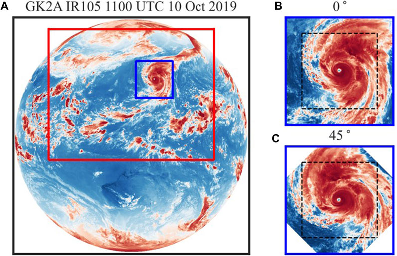
FIGURE 1. Example of extracting TC images from original satellite images to be used for model development. In (A), the black box is GK2A’s full disk area, the red box is COMS’s Northern Hemisphere area, and the blue box is the extracted TC area. In (B,C), the dashed black boxes represent the final images used for training, and the numbers at the top of the panels indicate the angles of rotation to the left. This image was taken at 11:00 UTC on 10 October 2019, using the GK2A IR105 channel.

TABLE 1

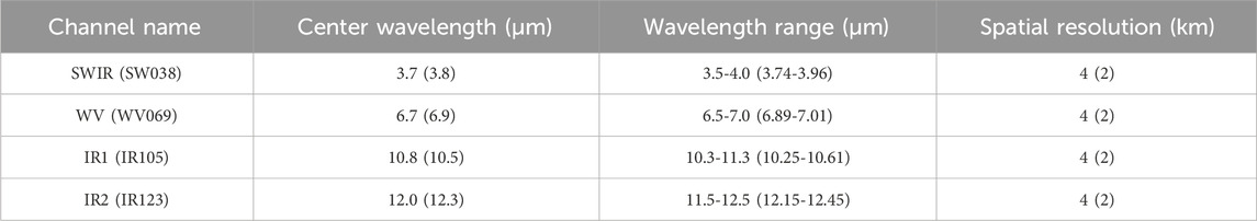
TABLE 1. Summary of the channels, center wavelengths, wavelength ranges, and spatial resolutions of the COMS and GK2A satellite imagery used in this study. The columns are arranged by COMS (GK2A) order.

The COMS data cover the period from April 2011 to June 2019, while the GK2A data used in this study cover the period from July 2019 to December 2021. We considered only TCs occurring in the western North Pacific during these periods. To prevent data leakage, different training and test datasets must be used (Kaufman et al., 2012). Accordingly, for the pre-trained model, we used the COMS data from April 2011 to December 2016 and from January 2017 to June 2019 as training and validation datasets, respectively, while for transfer learning, we used the GK2A 2019, 2020, and 2021 data as training, validation, and test datasets, respectively.

3 Materials and methods

3.1 Data preprocessing

Class imbalance, a situation in which one class has a significantly smaller volume of data than another, is considered one of the most formidable challenges in machine learning (Taherkhani et al., 2020). Buda et al. (2018) showed that data imbalance affected the performance of CNNs and used various data-based methods, such as oversampling, to tackle this problem. In this study, to balance the data, we divided the data into 10-knot intervals and ensured that the percentage of each bin is no more than 25% of the total data. In other words, if a particular bin is more than 25% of the total data, we randomly removed the excess. We also applied an oversampling method that increases the number of samples in a bin by rotating all images, ensuring that the number of all bins is close to twice the size of the largest bin. Bins with fewer data require more rotations at smaller angles. The smallest angle of rotation used is 1°.

To investigate the impact of rotation-based data augmentation on model performance, we compare the root mean square error (RMSE) for models trained on the original COMS data and augmented data, respectively, for GK2A validation data. The results showed that the model using the augmented COMS data had the RMSE of 13.67 knots, which was a 37.64% reduction compared to the model (21.92 knots) using the original data alone.

Because rotating TC images resulted in white space, as shown in Figure 1C, we needed to crop them to remove the white space. To crop to 303 × 303 pixels (black dashed line in Figures 1B, C), we needed to extract TCs with a minimum size of 429 × 429 pixels (blue line in Figure 1A) from the original satellite images. Since TC images are provided as digital counts, we converted them to brightness temperature using the brightness correction table provided by the National Meteorological Satellite Center.¹ Due to the different spatial resolutions of the two satellite datasets, we interpolated the GK2A data to make them equal to the COMS resolution.

After data balancing, the TC images become 303 × 303 pixels (i.e., 1,212 × 1,212 km), and then the image size becomes 101 × 101 pixels by upscaling with bilinear interpolation for computational efficiency. We combined the four infrared channels into one and normalized them using the maximum and minimum values within them. This method is helpful for CNN spatial pattern learning because it can capture the relative pattern distribution between channels. The data balancing, upscaling, and normalizing methods followed Lee et al. (2019a). We also normalized the label data from 0 to 1 (Baek et al., 2022) by dividing it by the maximum TC intensity (125 knots) among TCs that occurred from 2011 to 2020 to improve model convergence and generalization. To check that this maximum value is a reliable indicator even for future TCs with extreme intensities, we conducted sensitivity experiments in which we removed TC data with intensities above 120 knots from the train data and then estimated intensities of the removed TC data using different maximums (105, 119, 145 knots). The results show that the RMSEs for each experiment are 22.4, 15.44, and 24.13, respectively. This suggests that the choice of maximum value is sensitive to the performance of TC intensity estimation and the current method of using the true maximum in the data is the best way to estimate future extreme TCs.

Table 2 shows the numbers of COMS and GK2A images before and after data balancing. For the model to estimate TC intensity by learning additional data from 6 h earlier, the input data needed to include satellite imagery and TC intensity from 6 h earlier in addition to current satellite imagery. Due to computer memory issues, we reduced the augmentation of COMS data (parentheses in Table 2), as it would have otherwise doubled the amount of data compared to using current satellite data alone.

TABLE 2

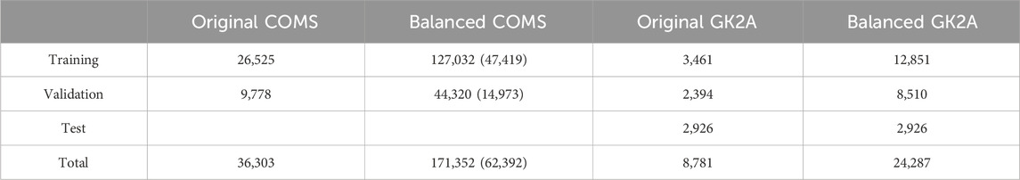
TABLE 2. Numbers of COMS and GK2A images used to develop the model. The numbers in parentheses represent operational models using information from 6 h earlier.

3.2 CNN model

CNNs are some of the most frequently used deep learning algorithms for many computer vision problems, such as digit identification and object recognition. A CNN consists of numerous processing layers to extract “features,” or increasingly abstract representations of input data, and fit them to target categories for classification tasks or to a target value for regression tasks (Chen et al., 2019a). The main advantage of CNNs is their weight-sharing feature, which reduces the number of trainable network parameters and subsequently aids in improving generalization and preventing overfitting (Alzubaidi et al., 2021).

The three main components of a CNN are convolutional layers, pooling layers, and the fully connected layer. Using a convolutional kernel in the convolutional layer reduces the number of parameters in the network and obviates the need to use a one-to-one connection between all pixel units (Hadji and Wildes, 2018). Pooling layers allow the detection of more abstract features and spatial contexts across scales and reduce the computational load and the risk of overfitting by reducing the number of model parameters (Kattenborn et al., 2021). The fully connected layers take in the mid- and low-level features and produce high-level abstraction, which corresponds to the final layers in a typical neural network (Alzubaidi et al., 2021).

The models for estimating TC intensity consisted of two to five convolutional blocks (CBs), including convolutional, activation, and pooling layers. The structure of each model is shown in Table 3. Sensitivity experiments showed that the optimal number of CBs was three. Figure 2 shows the structure of a model using only current satellite images and an operational model that additionally used satellite images and TC intensity information from 6 h earlier. For the former model, the input consisted of four-channel images, and the output was TC intensity. The latter consisted of three input layers (current four-channel images, images from 6 h earlier, and TC intensity from 6 h earlier) and one output layer (current TC intensity).

TABLE 3

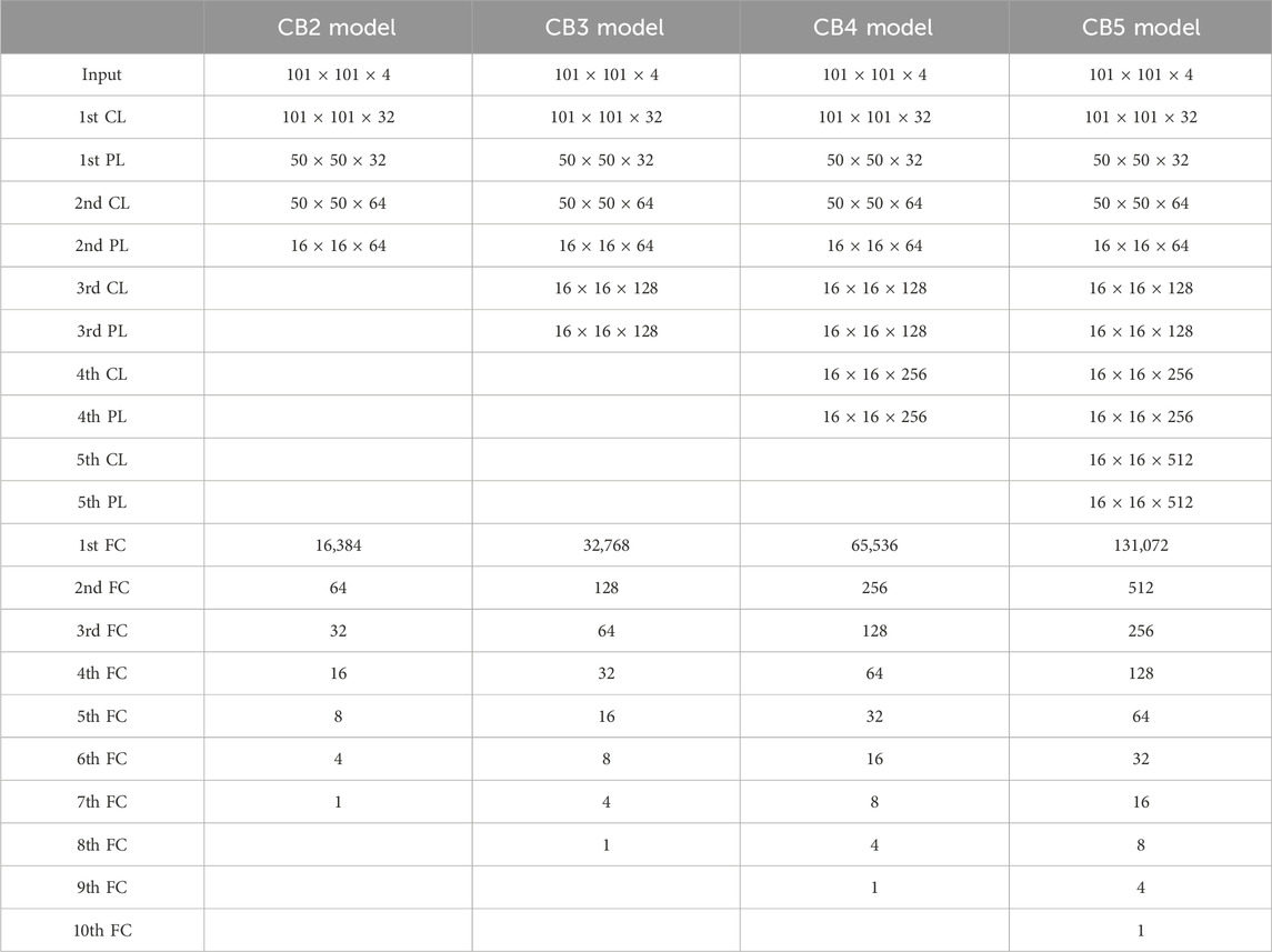
TABLE 3. Architectures of the CB2, CB3, CB4, and CB4 models, consisting of two, three, four, and five convolutional blocks (CBs), respectively. CL, PL, and FC represent the convolutional layer, the pooling layer, and the fully connected layer, respectively.

FIGURE 2

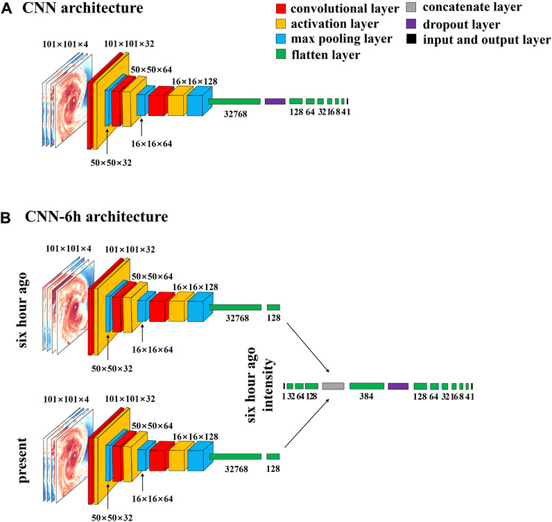
FIGURE 2. Architectures of (A) the CNN model using only current TC images and (B) the operational CNN model using TC images and intensity information from 6 h earlier as additional inputs. In (A), the current satellite images of four channels are inputted as a single input layer. In (B), the current four-channel satellite images and those from 6h earlier, along with TC intensity information from 6h earlier, are inputted through three separate input layers. The meanings of the colors in the layers are shown in the top right corner of the figure.

3.3 Transfer learning model and experimental design

CNNs learn domain-specific features at the top of the network and general features (such as colors and edges) at the bottom of the network (Karpathy et al., 2014). When applying transfer learning to a CNN, the bottom of the pre-trained model is frozen, while the top is trained in the target task. The layer to be trained with the target task (target layer) typically uses randomly initialized parameters (Yosinski et al., 2014). The parameters of the pre-trained model layers are either fine-tuned or frozen. Fine-tuning updates the parameters for new tasks, while frozen parameters are not updated. The choice between fine-tuned and frozen parameters depends on the size of the dataset and the number of parameters (Yosinski et al., 2014). If the target dataset is small and the number of parameters is large, keeping the features frozen is a better choice. On the other hand, if the target dataset is large or the number of parameters is small—and, thus, overfitting is not a concern—performance can be improved by fine-tuning the parameters for new tasks.

Since effective transfer learning methods differ depending on the nature of the data, we conducted sensitivity experiments on three transfer learning methods: fine-tuning, frozen, and frozen–fine-tuning. In the fine-tuning and frozen methods, the parameters of the target layer were randomly initialized. In the frozen–fine-tuning method, the parameters of the pre-trained model were frozen, and the target layers were fine-tuned. The aim of the latter was to examine whether it would be helpful to use the parameters of a model pre-trained with COMS as initial values for the target layer.

We conducted sensitivity experiments to determine the optimal number of CBs for the three transfer learning methods. The transfer learning experiments are denoted by the first two letters of the model’s name (TL), and frozen–fine-tuning, frozen, and fine-tuning are labeled “FFT,” “F,” and “FT,” respectively. The number of CBs used in each model is indicated at the end of the model’s name. The operational models, which additionally used satellite images and TC intensity information from 6 h ago, are indicated by “-6h” at the end of each model’s name. GK2A-only experiments without transfer learning, which were conducted to compare the performance of models with and without transfer learning, are labeled “GO.”

In the transfer learning experiments, we increased the number of layers by one to determine up to which layer it was most effective to keep the parameters of the pre-trained model frozen or fine-tune them. The sensitivity experiments are summarized in Table 4.

TABLE 4

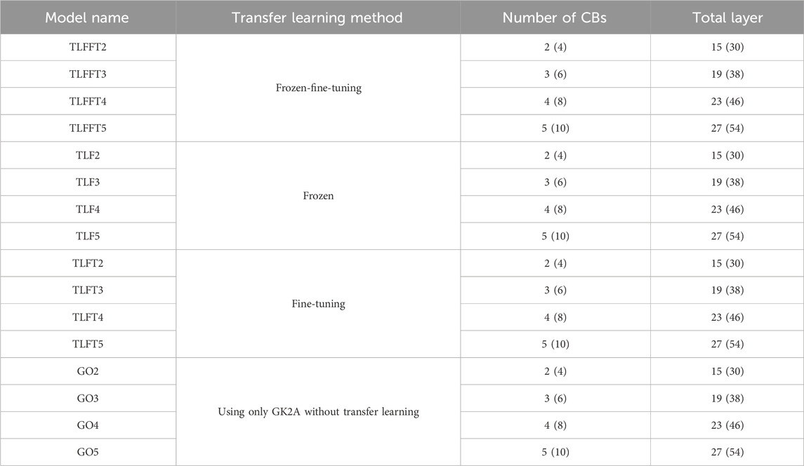
TABLE 4. Summary of the sensitivity experiments conducted in this study. For each experiment, the models’ names and numbers of CB layers and total layers are shown separately for the original models and the operational models using TC information from 6 h earlier (the latter are indicated in parentheses). The experimental names of the operational models are not indicated, but they can be recreated by adding “-6h” to the end of the model names in the first column. For example, TLFFT2 becomes TLFFT2-6h in the operational model experiment.

3.4 Hyperparameter tuning

Finding a suitable set of hyperparameters, such as the size and number of filters in the convolutional layers and the depth of the CBs, is important because it has a significant impact on the performance of machine learning algorithms (Li et al., 2018). We optimized the number of CBs, kernel size, dropout rate, and learning rate by performing hyperparameter tuning. As the depth of the CBs increases, the number of hyperparameters and the weights increase, which can lead to model overfitting, while a shallower depth can lead to underfitting (Baek et al., 2022). Compared to large filters, small filters in a model are better able to capture the local features of an input image, while large filters are better able to extract an input image’s general pattern. Although a small filter may extract a great deal of information from the input data, it may be necessary for the model to learn through a deeper convolutional layer, as it slows down the rate at which the dimensions are reduced (LeCun et al., 1989; Lee et al., 2019a; Baek et al., 2022). Dropout is a widely used technique for generalizing a model by randomly dropping neurons during each training epoch. Adjusting the learning rate values can reduce loss, improve accuracy, and control the total time required for network training (Ismail et al., 2019).

All models used in this study have the same range of hyperparameter tuning. The ranges of the number of CBs, filter size, learning rate, and dropout rate were [2, 3, 4, 5], [3, 5, 7, 9], [10⁻³, 10⁻⁴, 10⁻⁵, 10⁻⁶], and [0.25, 0.5, 0.75], respectively. The sensitivity experiments (see Section 4.1) showed that models with three CBs performed the best. For this reason, Table 5 shows only the hyperparameters of these models (i.e., TLFFT3, TLFFT3-6h, GO3, and GO3-6h). The convolutional layers of all models used the same padding and ReLU activation function. The adaptive momentum gradient descent optimizer and the mean squared error loss function were used for model training and optimization. The total number of training epochs was 50, and the number of early stopping epochs was 20, which helped reduce overfitting. The experiments were conducted using tensorflow as the deep learning framework.

TABLE 5

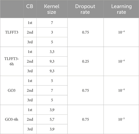
TABLE 5. Optimal kernel size, dropout rate, and learning rate used for the best-performing models with (TFFFT3 and TLFFT3-6h) and without (GO3 and GO3-6h) transfer learning. TLFFT3-6h and GO3-6h represent operational models using TC images and intensities from 6h earlier as additional inputs. The kernel size is shown for the first, second, and third convolutional blocks (CBs), and the number after the comma is the kernel size for the CB using 6 h earlier image as input.

4 Results

4.1 Sensitivity experiments

In this subsection, we present the results of the sensitivity experiments conducted to select the optimal transfer learning method, number of CBs, and number of frozen or fine-tuned layers. Model performance was evaluated based on the GK2A validation data using correlation coefficients (r), mean absolute error (MAE), RMSE, and bias. Among all possible experimental combinations, the frozen–fine-tuning model with three CBs and eight frozen layers (TLFFT3) showed the best performance. As an example, Figure 3 compares the performance of the three transfer learning methods (frozen–fine-tuning, fine-tuning, and frozen) as a function of the number of frozen or fine-tuned layers for models with three CBs. The frozen–fine-tuning method (black lines) exhibited the best overall performance and produced the best results when up to eight layers of the model were frozen (yellow symbol). The frozen–fine-tuning method relies more heavily on the parameters of the pre-trained model than the other methods because it uses them as initial values for all layers. Therefore, this result suggests that the pre-trained model’s task and the new target task (i.e., the COMS and GK2A data) were similar.

FIGURE 3

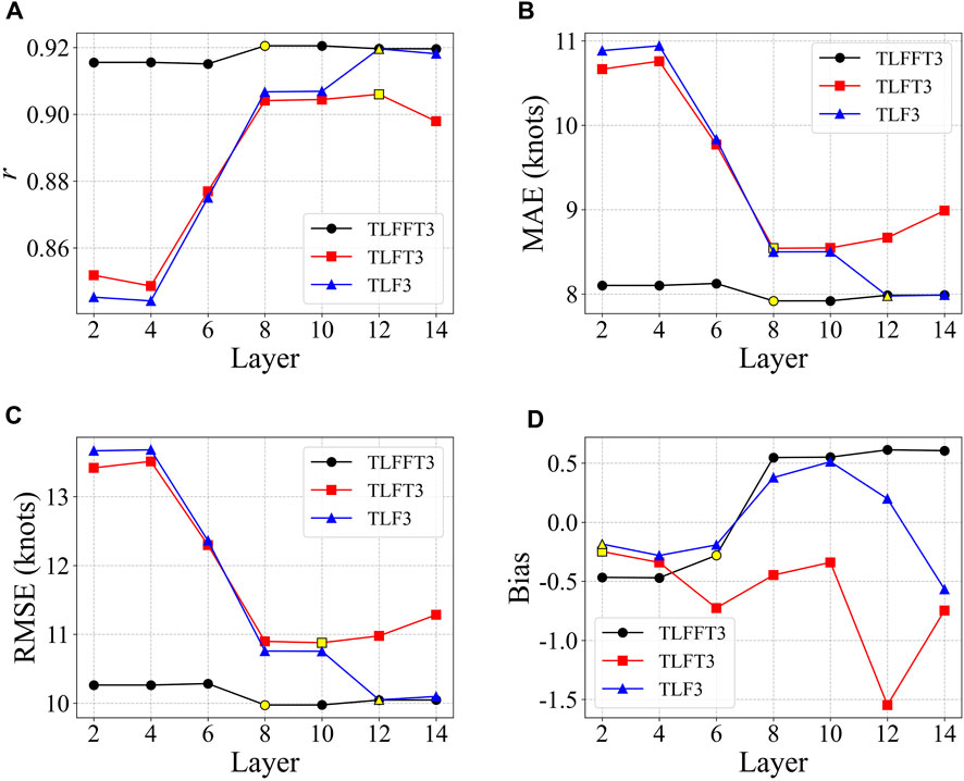
FIGURE 3. Comparison of the performance of the three transfer learning methods (TLFFT3, frozen–fine-tuning; TLFT3, fine-tuning; and TLF3, frozen) in terms of (A) correlation coefficients (r), (B) mean absolute error (MAE), (C) root mean square errors (RMSE), and (D) bias. Performance was evaluated based on the number of frozen (or fine-tuned) layers for models with three CBs. The yellow symbols indicate the best performance in each experiment.

Figure 3 also shows that TLFFT3 exhibited relatively little variation in r, MAE, and RMSE according to the number of frozen or fine-tuned layers compared to the fine-tuning (TLFT3) and frozen (TLF3) models, suggesting that it had consistently good performance. In the TLFFT3, TLFT3, and TLF3 experiments, the best performance was achieved when 8–12 layers were frozen or fine-tuned, suggesting that freezing or fine-tuning the layers of the pre-trained model up to at least the third CB (eighth layer) is helpful for TC intensity estimation. In the TLFT3 experiment, the RMSE tended to increase as the number of fine-tuned layers increased (10–14 layers). This is likely due to the limited size of the GK2A dataset used, which may result in overfitting if too many layers of the pre-trained model are fine-tuned.

Figure 4 compares the performance of the best transfer learning model (i.e., frozen–fine-tuning) as a function of the number of frozen layers and the number of CBs. Using three CBs (red lines) achieved the best performance, suggesting that too few CBs can prevent the network from learning sufficient data, while too many CBs can lead to overfitting. In all CB sensitivity experiments, the best performance (yellow symbols) was achieved when freezing layers up to (and including) the last CB of each model (i.e., the second, third, fourth, and fifth CBs of the CB2, CB3, CB4, and CB5 models, respectively), except for bias.

FIGURE 4

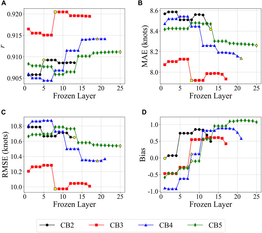
FIGURE 4. Comparison of performance as a function of the number of convolutional blocks (CBs) in terms of (A) correlation coefficients (r), (B) mean absolute error (MAE), (C) root mean square errors (RMSE), and (D) bias. Performance was evaluated based on the number of frozen layers in the frozen–fine-tuning model. The yellow symbols indicate the best performance in each experiment. CB2, CB3, CB4, and CB5 represent models with two, three, four, and five CBs and 15, 19, 23, and 27 layers, respectively.

4.2 Effect of using transfer learning

In this subsection, we compare the performance of the best-performing models with and without transfer learning (TLFFT3 and GO3, respectively) using GK2A validation and test data (Figure 5). TLFFT3 consistently outperformed GO3 in all evaluation metrics in both the validation and test datasets, with its RMSEs being lower by 23.54% and 20.16% than those of GO3 in the validation and test datasets, respectively.

FIGURE 5

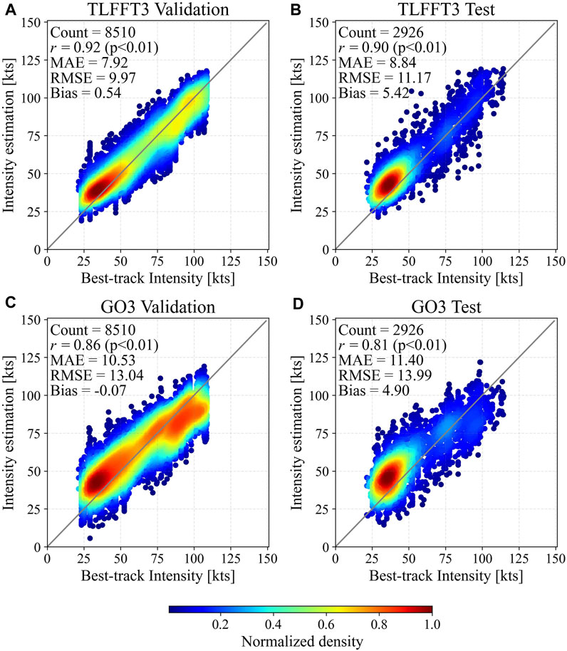
FIGURE 5. Density scatter plots of TC intensity estimation for GK2A validation (A,C) and test (B,D) data using the TLFFT3 (A,B) and GO3 models (C,D). In each panel, the x-axis shows the best-track TC intensity, and the y-axis shows the intensity predicted by the models. The upper left corner of each panel shows the number of data (Count), correlation coefficient (r), mean absolute error (MAE), root mean square error (RMSE), and bias.

We evaluated the stability and performance of the two models (TLFFT3 and GO3) based on the changes in loss and R² during the training and validation iterations (Figure 6). Loss measures the difference between the values predicted by the model and the actual data, while R² quantifies how well a regression model fits the data by indicating the proportion of the dependent variable’s variance explained by the model’s independent variables. In GO3, as the epochs increased, the validation loss became considerably greater than the training loss (solid and dashed red lines in Figure 6A). Moreover, the training loss of GO3 was considerably smaller than that of TLFFT3, but its validation loss was significantly larger. In contrast, TLFFT3 showed a small difference between validation and training losses in all epochs (solid and dashed black lines in Figure 6B), which did not change considerably as the epochs increased. A similar pattern was observed in R² (Figure 6B). These results suggest that the TLFFT3 model was stable and performed well, while the GO3 model was characterized by overfitting.

FIGURE 6

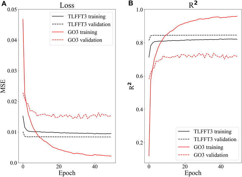
FIGURE 6. Comparison between the TLFFT3 and GO3 models in terms of (A) loss and (B) R² for the training and validation data. The black and red lines represent TLFFT3 and GO3, respectively, and the solid and dashed lines indicate the training and validation data, respectively.

A time series comparing the estimates of the two models with the best-track data for three TC cases also showed that the model with transfer learning (TLFFT3) outperformed the model without transfer learning (GO3) (Figure 7). For example, the intensities of In-Fa (2,106) and Chanthu (2,114) estimated by GO3 were frequently significantly higher or lower than the best-track values (Figures 7A, B). This seems to have been the result of overfitting. In contrast, TLFFT3 provided relatively consistent intensity estimates for both TCs. On the other hand, both models estimated the intensity of Mindulle (Figure 7C) more consistently than in the case of the other two TCs, with no significant difference in performance between them.

FIGURE 7

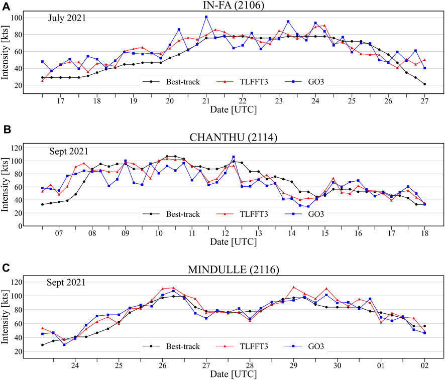
FIGURE 7. Time series of TC intensity estimated by the TLFFT3 and GO3 models, along with KMA best-track data for the 2021 TCs (A) In-Fa, (B) Chanthu, and (C) Mindulle. In each graph, the black line represents the best-track data, the red line indicates the intensity estimated by the TLFFT3 model, and the blue line shows the intensity estimated by the GO3 model. The month and year in which each TC occurred are shown in the upper left corner of each panel. The x-axis in each plot is marked with lines indicating 12-h intervals, and dates are shown at 00:00 UTC points.

4.3 Performance of operational models

For operational models, we compared the performance of the best-performing models with and without transfer learning (TLFFT3-6h and GO3-6h, respectively) to evaluate the impact of transfer learning on TC intensity estimates (Figure 8). Both operational models showed a significant performance improvement over the respective original models (TLFFT3 and GO3), which used only current TC images. Notably, both models showed r values exceeding 0.98 and MAEs lower than 3.24 in all training and validation periods, which represent considerably better performance than that of original models (compare Figures 5, 8). This suggests that using information from 6 h earlier in operational models is very helpful in estimating current TC intensity, which tends to vary over time.

FIGURE 8

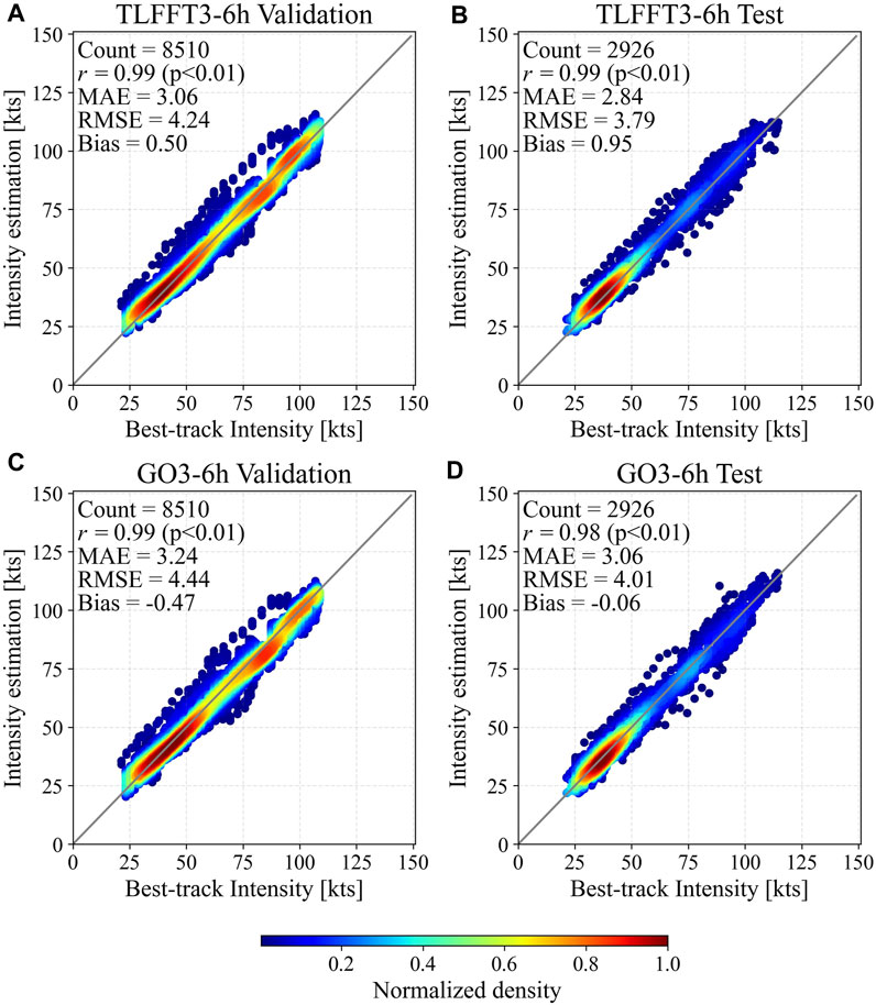
FIGURE 8. Density scatter plots of TC intensity estimation for GK2A validation (A, C) and test (B, D) data using the TLFFT3-6h (A, B) and GO3-6h models (C, D). In each panel, the x-axis shows the best-track TC intensity, and the y-axis shows the intensity predicted by the models. The upper left corner of each panel shows the number of data (Count), correlation coefficient (r), mean absolute error (MAE), root mean square error (RMSE), and bias.

A comparison between TLFFT3-6h and GO3-6h showed that the former outperformed the latter in all evaluation metrics, with RMSEs lower by 5.49% and 4.5% for the test and validation data, respectively. This suggests that the transfer learning technique was still effective in the operational TLFFT3 model (TLFFT3-6h). It should be noted that the reduction in RMSE through transfer learning was considerably smaller in the operational model (5.49%) than in the original model (20.16%) for the test data, but this difference is attributed to the inherently lower error of the GO3-6h model itself making further improvement difficult.

In general, validation performance is better than the test as seen in the most cases in Figure 5. Because the model’s hyperparameters will have been tuned specifically for the validation dataset. However, Figure 8 shows the opposite results. This is because if there is not enough data for testing, there may be bias in the data, which can sometimes lead to test results performing better than validation. In fact, other studies have also reported that test results sometimes perform better than validation (Baek et al., 2022; Tong et al., 2023). Our data was divided by year to avoid data leakage and, due to the limited number of available data, the sample size of the test dataset is small (only 1 year). Since characteristics of TCs vary from year to year, tests using only 1 year’s data may be biased.

5 Discussion and conclusion

GK2A, the successor of COMS (Korea’s first geostationary satellite), was launched in July 2019 and has therefore not accumulated sufficient data. To address this problem, we applied the transfer learning method to models pre-trained on COMS data to estimate TC intensity. To our knowledge, no other study has applied transfer learning to TC intensity estimation using these data. To select a suitable transfer learning method, we evaluated the performance of several methods based on GK2A validation data. The frozen–fine-tuning method, which freezes the parameters of the pre-trained model and fine-tunes the subsequent layers, showed the best performance. This suggests that using the parameters of the pre-trained model as a starting point in all layers is advantageous for TC intensity estimation. The sensitivity experiments conducted to determine the optimal number of CBs showed that the use of three CBs was the most appropriate. When tested using 2021 TC data, the TLFFT3 model, which had both frozen and fine-tuned parameters and three CBs, yielded an RMSE lower by 20.16% than that of the model using GK2A data alone (GO3). In the operational model using additional satellite images and TC intensity information from 6 h earlier, transfer learning further reduced the RMSE by 5.49%. Our results show that the use of transfer learning for GK2A and COMS data can enhance TC intensity estimations based on CNNs. Specifically, the findings suggest that the frozen–fine-tuning method is the most suitable. However, this conclusion relies heavily on the similarity between the two datasets used. To check the similarity of the COMS and GK2A data, we calculated the r values and mean absolute difference (MAD) of the brightness temperatures of two datasets for a TC at 08:00 UTC on 2 October 2019 (Figure 9). All data from the four channels (IR1, IR2, SWIR, and WV) showed high correlations (more than 0.97) between the two datasets and low MADs (2.95, 3.34, 2.45, and 6.68 K, respectively), indicating that the two datasets are very similar.

FIGURE 9

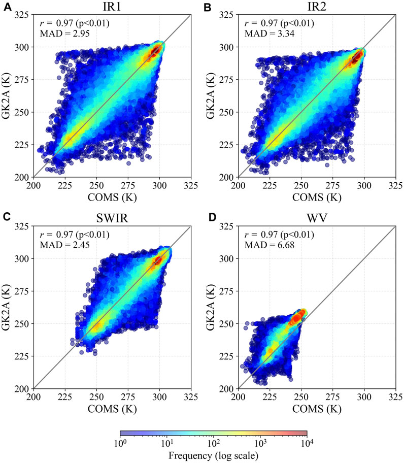
FIGURE 9. Scatter plots of brightness temperatures frequency for (A) IR1, (B) IR2, (C) SWIR, and (D) WV channels of COMS and GK2A, including data distribution information. The units are in Kelvins. Correlation coefficient (r) and mean absolute difference (MAD) are shown in the upper left corner of the figure.

Since the two data sets are very similar, we investigated the difference in performance when using transfer learning and when training a model on the combined COMS and GK2A datasets. In this experiment, we compared the performance using the original data without data augmentation due to computer memory issues. The results show that in GK2A validation data, the RMSE for the combined-data model was 18.86 knots, while for the transfer learning model it was 15.68 knots. The error of the transfer learning model was 16.6% lower than that of the combined-data model. This indicates that transfer learning model performs better than the combined-data model.

Although the GK2A and COMS datasets differ in terms of the sensors, resolutions, and algorithms used, the fact that data from similar channels exhibit a high degree of similarity is of great importance. This is because the developed approach can be applied to other satellite data with similar characteristics, such as Geostationary Operational Environmental Satellites (GOES), Himawari satellites, and geostationary meteorological satellites (Meteosat). Transfer learning is a powerful tool because it leverages information learned from pre-trained models, which helps conserve computer resources, prevent overfitting, and overcome data scarcity. Given that currently operational geostationary satellites have a lifespan of approximately 10 years, transfer learning may represent a new breakthrough in satellite utilization research by enabling the use of diverse satellite data to overcome data scarcity.

Data availability statement

The original contributions presented in the study are included in the article, further inquiries can be directed to the corresponding author.

Author contributions

HJ: Conceptualization, Data curation, Formal Analysis, Investigation, Methodology, Validation, Writing–original draft, Writing–review and editing. Y-HB: Data curation, Formal Analysis, Writing–review and editing, Methodology. I-JM: Conceptualization, Formal Analysis, Investigation, Methodology, Data curation, Supervision, Writing–review and editing, Resources. JL: Methodology, Conceptualization, Data curation, Formal Analysis, Writing–review and editing. E-HS: Funding acquisition, Project administration, Writing–review and editing.

Funding

The author(s) declare financial support was received for the research, authorship, and/or publication of this article. This work was funded by the Korea Meteorological Administration’s Research and Development Program “Technical Development on Weather Forecast Support and Convergence Service using Meteorological Satellites“ under Grant (KMA2020-00120) and Korea Institute of Marine Science and Technology Promotion(KIMST) funded by the Korea Coast Guard(RS-2023-00238652, Integrated Satellite-based Applications Development for Korea Coast Guard).

Conflict of interest

The authors declare that the research was conducted in the absence of any commercial or financial relationships that could be construed as a potential conflict of interest.

The author(s) declared that they were an editorial board member of Frontiers, at the time of submission. This had no impact on the peer review process and the final decision.

Publisher’s note

All claims expressed in this article are solely those of the authors and do not necessarily represent those of their affiliated organizations, or those of the publisher, the editors and the reviewers. Any product that may be evaluated in this article, or claim that may be made by its manufacturer, is not guaranteed or endorsed by the publisher.

Footnotes

¹Online. [Available]: http://nmsc.kma.go.kr/html/homepage/ko/main.do

References

Alzubaidi, L., Zhang, J., Humaidi, A. J., Al-Dujaili, A., Duan, Y., Al-Shamma, O., et al. (2021). Review of deep learning: concepts, CNN architectures, challenges, applications, future directions. J. Big Data 8, 53–74. doi:10.1186/s40537-021-00444-8

PubMed Abstract | CrossRef Full Text | Google Scholar

Aslan, M. F., Unlersen, M. F., Sabanci, K., and Durdu, A. (2021). CNN-based transfer learning–BiLSTM network: a novel approach for COVID-19 infection detection. Appl. Soft Comput. 98, 106912. doi:10.1016/j.asoc.2020.106912

PubMed Abstract | CrossRef Full Text | Google Scholar

Baek, J.-J., and Choi, M.-H. (2012). Availability of land surface temperature from the COMS in the Korea Peninsula. J. Korea Water Resour. Assoc. 45, 755–765. doi:10.3741/JKWRA.2012.45.8.755

CrossRef Full Text | Google Scholar

Baek, Y.-H., Moon, I.-J., Im, J., and Lee, J. (2022). A novel tropical cyclone size estimation model based on a convolutional neural network using geostationary satellite imagery. Remote Sens. 14, 426. doi:10.3390/rs14020426

CrossRef Full Text | Google Scholar

Baik, J., and Choi, M. (2015). Evaluation of geostationary satellite (COMS) based Priestley–Taylor evapotranspiration. Agric. Water Manag. 159, 77–91. doi:10.1016/j.agwat.2015.05.017

CrossRef Full Text | Google Scholar

Buda, M., Maki, A., and Mazurowski, M. A. (2018). A systematic study of the class imbalance problem in convolutional neural networks. Neural Netw. 106, 249–259. doi:10.1016/j.neunet.2018.07.011

PubMed Abstract | CrossRef Full Text | Google Scholar

Cao, J., Chen, Z., and Wang, B. (2016). “Deep convolutional networks with superpixel segmentation for hyperspectral image classification,” in 2016 IEEE International Geoscience and Remote Sensing Symposium (IGARSS), Beijing, China, 10-15 July 2016 (IEEE), 3310–3313. doi:10.1109/IGARSS.2016.7729856

CrossRef Full Text | Google Scholar

Chen, B., Chen, B.-F., and Lin, H.-T. (2018). “Rotation-blended CNNs on a new open dataset for tropical cyclone image-to-intensity regression,” in Proceedings of the 24th ACM SIGKDD International Conference on Knowledge Discovery and Data Mining, New York, NY, USA (ACM), 90–99. doi:10.1145/3219819.3219926

CrossRef Full Text | Google Scholar

Chen, B.-F., Chen, B., Lin, H.-T., and Elsberry, R. L. (2019a). Estimating tropical cyclone intensity by satellite imagery utilizing convolutional neural networks. Weather Forecast 34, 447–465. doi:10.1175/WAF-D-18-0136.1

CrossRef Full Text | Google Scholar

Chen, G., Chen, Z., Zhou, F., Yu, X., Zhang, H., and Zhu, L. (2019b). “A semisupervised deep learning framework for tropical cyclone intensity estimation,” in 2019 10th International Workshop on the Analysis of Multitemporal Remote Sensing Images (MultiTemp), Shanghai, China, 5-7 Aug. 2019 (IEEE), 1–4. doi:10.1109/Multi-Temp.2019.8866970

CrossRef Full Text | Google Scholar

Chen, Z., Chen, G., Zhou, F., Yang, B., Wang, L., Liu, Q., et al. (2020). “A novel general semisupervised deep learning framework for classification and regression with remote sensing images,” in IGARSS 2020 - 2020 IEEE International Geoscience and Remote Sensing Symposium, Waikoloa, HI, USA, 26 Sept.-2 Oct. 2020 (IEEE), 1323–1326. doi:10.1109/IGARSS39084.2020.9323932

CrossRef Full Text | Google Scholar

Chen, Z., and Yu, X. (2021). A novel tensor network for tropical cyclone intensity estimation. IEEE Trans. Geosci. Remote Sens. 59, 3226–3243. doi:10.1109/TGRS.2020.3017709

CrossRef Full Text | Google Scholar

Cho, A.-R., and Suh, M.-S. (2013). Evaluation of land surface temperature operationally retrieved from Korean geostationary satellite (COMS) data. Remote Sens. 5, 3951–3970. doi:10.3390/rs5083951

CrossRef Full Text | Google Scholar

Choi, Y.-Y., Suh, M.-S., and Park, K.-H. (2014). Assessment of surface urban heat islands over three megacities in East Asia using land surface temperature data retrieved from COMS. Remote Sens. 6, 5852–5867. doi:10.3390/rs6065852

CrossRef Full Text | Google Scholar

Combinido, J. S., Mendoza, J. R., and Aborot, J. (2018). “A convolutional neural network approach for estimating tropical cyclone intensity using satellite-based infrared images,” in 2018 24th International Conference on Pattern Recognition (ICPR), Beijing, China, 20-24 Aug. 2018 (IEEE), 1474–1480. doi:10.1109/ICPR.2018.8545593

CrossRef Full Text | Google Scholar

Deepak, S., and Ameer, P. M. (2019). Brain tumor classification using deep CNN features via transfer learning. Comput. Biol. Med. 111, 103345. doi:10.1016/j.compbiomed.2019.103345

PubMed Abstract | CrossRef Full Text | Google Scholar

Deo, R. V., Chandra, R., and Sharma, A. (2017). Stacked transfer learning for tropical cyclone intensity prediction. arXiv.org. Available at: 10.48550/arXiv.1708.06539 (Accessed August 16, 2023).

Google Scholar

Dvorak, V. F. (1975). Tropical cyclone intensity analysis and forecasting from satellite imagery. Mon. Weather Rev. 103, 420–430. doi:10.1175/1520-0493(1975)103<0420:TCIAAF>2.0.CO;2

CrossRef Full Text | Google Scholar

Dvorak, V. F. (1984). Tropical cyclone intensity analysis using satellite data, Vol. 11. Maryland: US Department of Commerce, National Oceanic and Atmospheric Administration, National Environmental Satellite, Data, and Information Service.

Google Scholar

Gorban, A. N., Mirkes, E. M., and Tyukin, I. Y. (2020). How deep should be the depth of convolutional neural networks: a backyard dog case study. Cogn. Comput. 12, 388–397. doi:10.1007/s12559-019-09667-7

CrossRef Full Text | Google Scholar

Hadji, I., and Wildes, R. P. (2018). What do we understand about convolutional networks? arXiv.org. Available at: https://arxiv.org/abs/1803.08834 (Accessed August 19, 2023).

Google Scholar

Ham, Y.-G., Kim, J.-H., and Luo, J.-J. (2019). Deep learning for multi-year ENSO forecasts. Nature 573, 568–572. doi:10.1038/s41586-019-1559-7

PubMed Abstract | CrossRef Full Text | Google Scholar

Hassan, S. M., Maji, A. K., Jasiński, M., Leonowicz, Z., and Jasińska, E. (2021). Identification of plant-leaf diseases using CNN and transfer-learning approach. Electronics 10, 1388. doi:10.3390/electronics10121388

CrossRef Full Text | Google Scholar

Huang, X., Peng, X., Fei, J., Cheng, X., Ding, J., and Yu, D. (2021). Evaluation and error analysis of official tropical cyclone intensity forecasts during 2005–2018 for the western North Pacific. J. Meteorol. Soc. Jpn. Ser. II 99, 139–163. doi:10.2151/jmsj.2021-008

CrossRef Full Text | Google Scholar

Imoto, K., Nakai, T., Ike, T., Haruki, K., and Sato, Y. (2019). A CNN-based transfer learning method for defect classification in semiconductor manufacturing. IEEE Trans. Semicond. Manuf. 32, 455–459. doi:10.1109/TSM.2019.2941752

CrossRef Full Text | Google Scholar

Ismail, A., Ahmad, S. A., Che Soh, A., Hassan, K., and Harith, H. H. (2019). Improving convolutional neural network (CNN) architecture (miniVGGNet) with batch normalization and learning rate decay factor for image classification. Int. J. Integr. Eng. 11, 51–59. doi:10.30880/ijie.2019.11.04.006

CrossRef Full Text | Google Scholar

Jiang, S., and Tao, L. (2022). Classification and estimation of typhoon intensity from geostationary meteorological satellite images based on deep learning. Atmos. (Basel). 13, 1113. doi:10.3390/atmos13071113

CrossRef Full Text | Google Scholar

Jiang, Y., Li, Y., and Zhang, H. (2019). Hyperspectral image classification based on 3-D separable ResNet and transfer learning. IEEE Geosci. Remote Sens. Lett. 16, 1949–1953. doi:10.1109/LGRS.2019.2913011

CrossRef Full Text | Google Scholar

Karpathy, A., Toderici, G., Shetty, S., Leung, T., Sukthankar, R., and Fei-Fei, L. (2014). “Large-scale video classification with convolutional neural networks,” in 2014 IEEE Conference on Computer Vision and Pattern Recognition, Columbus, OH, USA, 23-28 June 2014 (IEEE), 1725–1732. doi:10.1109/CVPR.2014.223

CrossRef Full Text | Google Scholar

Kattenborn, T., Leitloff, J., Schiefer, F., and Hinz, S. (2021). Review on convolutional neural networks (CNN) in vegetation remote sensing. ISPRS J. Photogramm. Remote Sens. 173, 24–49. doi:10.1016/j.isprsjprs.2020.12.010

CrossRef Full Text | Google Scholar

Kaufman, S., Rosset, S., Perlich, C., and Stitelman, O. (2012). Leakage in data mining. ACM Trans. Knowl. Discov. Data 6, 1–21. doi:10.1145/2382577.2382579

CrossRef Full Text | Google Scholar

Kim, M., Park, M.-S., Choi, Y., Kwon, M., and Jang, E. (2022). “CNN-based tropical cyclone intensity prediction using satellite inner-core feature extraction and reanalysis large-scale environment data,” in AGU fall meeting abstracts. Available at: https://ui.adsabs.harvard.edu/abs/2022AGUFM.A15E.04K/abstract (Accessed August 29, 2023).

Google Scholar

Kwon, M. (2012). Estimation and statistical characteristics of the radius of maximum wind of tropical cyclones using COMS IR imagery. Atmos. (Basel) 22, 473–481. doi:10.14191/Atmos.2012.22.4.473

CrossRef Full Text | Google Scholar

LeCun, Y., Boser, B., Denker, J., Henderson, D., Howard, R., Hubbard, W., et al. (1989). “Handwritten digit recognition with a back-propagation network,” in Advances in neural information processing systems. Available at: https://papers.nips.cc/paper/1989/hash/53c3bce66e43be4f209556518c2fcb54-Abstract.html (Accessed August 19, 2023).

Google Scholar

Lee, J., Im, J., Cha, D.-H., Park, H., and Sim, S. (2019a). Tropical cyclone intensity estimation using multi-dimensional convolutional neural networks from geostationary satellite data. Remote Sens. 12, 108. doi:10.3390/rs12010108

CrossRef Full Text | Google Scholar

Lee, J., Yoo, C., Im, J., Shin, Y., and Cho, D. (2020). Multi-task learning based tropical cyclone intensity monitoring and forecasting through fusion of geostationary satellite data and numerical forecasting model output. Korean J. Remote Sens. 36, 1037–1051. doi:10.7780/kjrs.2020.36.5.3.4

CrossRef Full Text | Google Scholar

Lee, Y., Jung, C., and Kim, S. (2019b). Spatial distribution of soil moisture estimates using a multiple linear regression model and Korean geostationary satellite (COMS) data. Agric. Water Manag. 213, 580–593. doi:10.1016/j.agwat.2018.09.004

CrossRef Full Text | Google Scholar

Lee, Y.-J., Hall, D., Liu, Q., Liao, W.-W., and Huang, M.-C. (2021). Interpretable tropical cyclone intensity estimation using Dvorak-inspired machine learning techniques. Eng. Appl. Artif. Intell. 101, 104233. doi:10.1016/j.engappai.2021.104233

CrossRef Full Text | Google Scholar

Lee, Y.-K., and Kwon, M. (2015). An estimation of the of tropical cyclone size using COMS infrared imagery. Atmos. (Basel) 25, 569–573. doi:10.14191/Atmos.2015.25.3.569

CrossRef Full Text | Google Scholar

Li, L., Jamieson, K., DeSalvo, G., Rostamizadeh, A., and Talwalkar, A. (2018). Hyperband: a novel bandit-based approach to hyperparameter optimization. J. Mach. Learn. Res. 18, 6765–6816. doi:10.48550/arXiv.1603.06560

CrossRef Full Text | Google Scholar

Li, Z., Guo, F., Li, Q., Ren, G., and Wang, L. (2020). An encoder–decoder convolution network with fine-grained spatial information for hyperspectral images classification. IEEE Access 8, 33600–33608. doi:10.1109/ACCESS.2020.2974025

CrossRef Full Text | Google Scholar

Liu, C.-C., Liu, C.-Y., Lin, T.-H., and Chen, L.-D. (2015). A satellite-derived typhoon intensity index using a deviation angle technique. Int. J. Remote Sens. 36, 1216–1234. doi:10.1080/01431161.2015.1009647

CrossRef Full Text | Google Scholar

Liu, X., Sun, Q., Meng, Y., Fu, M., and Bourennane, S. (2018). Hyperspectral image classification based on parameter-optimized 3D-CNNs combined with transfer learning and virtual samples. Remote Sens. 10, 1425. doi:10.3390/rs10091425

CrossRef Full Text | Google Scholar

Pan, S. J., Tsang, I. W., Kwok, J. T., and Yang, Q. (2011). Domain adaptation via transfer component analysis. IEEE Trans. Neural Netw. 22, 199–210. doi:10.1109/TNN.2010.2091281

PubMed Abstract | CrossRef Full Text | Google Scholar

Pan, S. J., and Yang, Q. (2010). A survey on transfer learning. IEEE Trans. Knowl. Data Eng. 22, 1345–1359. doi:10.1109/TKDE.2009.191

CrossRef Full Text | Google Scholar

Pang, S., Xie, P., Xu, D., Meng, F., Tao, X., Li, B., et al. (2021). NDFTC: a new detection framework of tropical cyclones from meteorological satellite images with deep transfer learning. Remote Sens. 13, 1860. doi:10.3390/rs13091860

CrossRef Full Text | Google Scholar

Pineros, M. F., Ritchie, E. A., and Tyo, J. S. (2008). Objective measures of tropical cyclone structure and intensity change from remotely sensed infrared image data. IEEE Trans. Geosci. Remote Sens. 46, 3574–3580. doi:10.1109/TGRS.2008.2000819

CrossRef Full Text | Google Scholar

Piñeros, M. F., Ritchie, E. A., and Tyo, J. S. (2011). Estimating tropical cyclone intensity from infrared image data. Weather Forecast 26, 690–698. doi:10.1175/WAF-D-10-05062.1

CrossRef Full Text | Google Scholar

Pradhan, R., Aygun, R. S., Maskey, M., Ramachandran, R., and Cecil, D. J. (2018). Tropical cyclone intensity estimation using a deep convolutional neural network. IEEE Trans. Image Process. 27, 692–702. doi:10.1109/TIP.2017.2766358

PubMed Abstract | CrossRef Full Text | Google Scholar

Rahman, T., Chowdhury, M. E. H., Khandakar, A., Islam, K. R., Islam, K. F., Mahbub, Z. B., et al. (2020). Transfer learning with deep convolutional neural network (CNN) for pneumonia detection using chest X-ray. Appl. Sci. 10, 3233. doi:10.3390/app10093233

CrossRef Full Text | Google Scholar

Ritchie, E. A., Wood, K. M., Rodríguez-Herrera, O. G., Piñeros, M. F., and Tyo, J. S. (2014). Satellite-derived tropical cyclone intensity in the North Pacific Ocean using the deviation-angle variance technique. Weather Forecast 29, 505–516. doi:10.1175/WAF-D-13-00133.1

CrossRef Full Text | Google Scholar

Sanabia, E. R., Barrett, B. S., and Fine, C. M. (2014). Relationships between tropical cyclone intensity and eyewall structure as determined by radial profiles of inner-core infrared brightness temperature. Mon. Weather Rev. 142, 4581–4599. doi:10.1175/MWR-D-13-00336.1

CrossRef Full Text | Google Scholar

Taherkhani, A., Cosma, G., and McGinnity, T. M. (2020). AdaBoost-CNN: an adaptive boosting algorithm for convolutional neural networks to classify multi-class imbalanced datasets using transfer learning. Neurocomputing 404, 351–366. doi:10.1016/j.neucom.2020.03.064

CrossRef Full Text | Google Scholar

Tan, J., Yang, Q., Hu, J., Huang, Q., and Chen, S. (2022). Tropical cyclone intensity estimation using Himawari-8 satellite cloud products and deep learning. Remote Sens. 14, 812. doi:10.3390/rs14040812

CrossRef Full Text | Google Scholar

Tian, W., Huang, W., Yi, L., Wu, L., and Wang, C. (2020). A CNN-based hybrid model for tropical cyclone intensity estimation in meteorological industry. IEEE Access 8, 59158–59168. doi:10.1109/ACCESS.2020.2982772

CrossRef Full Text | Google Scholar

Tian, W., Zhou, X., Huang, W., Zhang, Y., Zhang, P., and Hao, S. (2022). Tropical cyclone intensity estimation using multidimensional convolutional neural network from multichannel satellite imagery. IEEE Geosci. Remote Sens. Lett. 19, 1–5. doi:10.1109/LGRS.2021.3134007

CrossRef Full Text | Google Scholar

Tong, B., Fu, J., Deng, Y., Huang, Y., Chan, P., and He, Y. (2023). Estimation of tropical cyclone intensity via deep learning techniques from satellite cloud images. Remote Sens. 15, 4188. doi:10.3390/rs15174188

CrossRef Full Text | Google Scholar

Wang, C., Zheng, G., Li, X., Xu, Q., Liu, B., and Zhang, J. (2022). Tropical cyclone intensity estimation from geostationary satellite imagery using deep convolutional neural networks. IEEE Trans. Geosci. Remote Sens. 60, 1–16. doi:10.1109/TGRS.2021.3066299

CrossRef Full Text | Google Scholar

Yang, J., Zhao, Y.-Q., and Chan, J. C.-W. (2017). Learning and transferring deep joint spectral–spatial features for hyperspectral classification. IEEE Trans. Geosci. Remote Sens. 55, 4729–4742. doi:10.1109/TGRS.2017.2698503

CrossRef Full Text | Google Scholar

Yeom, J.-M., Park, S., Chae, T., Kim, J.-Y., and Lee, C. S. (2019). Spatial assessment of solar radiation by machine learning and deep neural network models using data provided by the COMS MI geostationary satellite: a case study in South Korea. Sensors 19, 2082. doi:10.3390/s19092082

PubMed Abstract | CrossRef Full Text | Google Scholar

Yosinski, J., Clune, J., Bengio, Y., and Lipson, H. (2014). “How transferable are features in deep neural networks?,” in Advances in neural information processing systems, 27, 3320–3328. Available at: https://arxiv.org/abs/1411.1792 (Accessed August 19, 2023).

Google Scholar

Zhang, C.-J., Wang, X.-J., Ma, L.-M., and Lu, X.-Q. (2021). Tropical cyclone intensity classification and estimation using infrared satellite images with deep learning. IEEE J. Sel. Top. Appl. Earth Obs. Remote Sens. 14, 2070–2086. doi:10.1109/JSTARS.2021.3050767

CrossRef Full Text | Google Scholar

Zhang, Z., Yang, X., Wang, X., Wang, B., Wang, C., and Du, Z. (2022). A neural network with spatiotemporal encoding module for tropical cyclone intensity estimation from infrared satellite image. Knowledge-Based Syst. 258, 110005. doi:10.1016/j.knosys.2022.110005

CrossRef Full Text | Google Scholar

Zhao, Y., Zhao, C., Sun, R., and Wang, Z. (2016). A multiple linear regression model for tropical cyclone intensity estimation from satellite infrared images. Atmos. (Basel). 7, 40. doi:10.3390/atmos7030040

CrossRef Full Text | Google Scholar