Joint inversion of gravity and gravity gradient data using smoothed L0 norm regularization algorithm with sensitivity matrix compression

Improving efficiency and accuracy are critical issues in geophysical inversion. In this study, a new algorithm is proposed for the joint inversion of gravity and gravity gradient data. Based on the regularization theory, the objective function is constructed using smoothed L₀ norm (SL0), then the optimal solution is obtained by the non-linear conjugate gradient method. Numerical modeling shows that our algorithm is much more efficient than the conventional SL0 based on the sparse theory, especially when inverting large-scale data, and also has better anti-noise performance while preserving its advantage of high accuracy. Compressing the sensitivity matrices has further improved efficiency, and introducing the data weighting and the self-adaptive regularization parameter has improved the convergence rate of the inversion. Moreover, the impacts of the depth weighting, model weighting, and density constraint are also analyzed. Finally, our algorithm is applied to the gravity and gravity gradient measurements at the Vinton salt dome. The inverted distribution range, thickness, and geometry of the cap rock are in good agreement with previous studies based on geological data, drilling data, seismic data, etc., validating the feasibility of this algorithm in actual geological conditions.

1 Introduction

Gravity and gravity gradient data are critical for investigation in geoscience. In comparison, gravity data contain more low-frequency information about deep structures, while gravity gradient data contain more high-frequency information and are sensitive to density non-uniformity of shallow structures (Zhang et al., 2000; Beiki, 2010; Ma et al., 2012). Consequently, joint inversion using gravity and gravity gradient data could improve the reliability of the results and has been widely applied in recent years (e.g., Wu et al., 2012; Capriotti and Li, 2014; Paoletti et al., 2016; Qin et al., 2016; Geng et al., 2017; Wang et al., 2017; Zhao et al., 2018; Capriotti and Li, 2022; Wang et al., 2022; Liu et al., 2023).

Geophysical inversion is usually solved based on the regularization theory (Tikhonov and Arsenin, 1977), such as the smoothest inversion with L₂ norm minimization (Li and Oldenburg, 1998; Lelievre and Farquharson, 2013; Tu et al., 2022), the focusing inversion with non-L₂ norm minimization (Portniaguine and Zhdanov, 1999; Zhdanov, 2009; Gebre and Lewi, 2023; Rezaie, 2023), the combination of them using mixed norm (Kowalski and Torrésani, 2009; Pérez et al., 2017; Zhao et al., 2023), and the Markov random field (MRF) method (Bhatt et al., 2014; Guo et al., 2017; 2020). Another method is the smoothed L₀ norm (SL0) inversion (Mohimani et al., 2009), which approximates the discontinuous L₀ norm by a suitable continuous function and performs minimization. Meng (2016) proposed the SL0 sparse recovery inversion based on the sparse theory and concluded that when compared with the smoothest and the focusing inversion based on the regularization theory, this algorithm could obtain more accurate results with relatively sharp edge information. However, the SL0 sparse recovery (from now on we refer to it as the conventional SL0) involves the calculation of matrix inverse which limits its capability of processing large-scale data. Additionally, it constructs the joint inversion by overlaying gravity and gravity gradient data and, therefore, is sensitive to noise. The challenging question is whether and how joint inversion of gravity and gravity gradient data could be conducted using SL0 based on the regularization theory to lower its memory cost as well as improve its efficiency and anti-noise performance while preserving its accuracy.

There are many studies on improving the capability of processing large-scale gravity and gravity gradient data in inversion (e.g., Chen et al., 2012; Jing et al., 2019; Yin et al., 2023). Yao et al. (2003) proposed the geometric trellis theory, which only needs to calculate one part of the trellises and then derive the others according to the equivalence of shift and symmetry reciprocation. It is shown to compress the sensitivity matrix to lower calculation and memory cost of gravity and gravity gradient data joint inversion (Qin and Huang, 2016; Zhang et al., 2021), and thus worthy to be applied on the subsequent algorithm we proposed for further improvement.

In this study, we construct the objective function with SL0 based on the regularization theory to conduct joint inversion of gravity and gravity gradient data and obtain the optimal solution using the non-linear conjugate gradient method. Moreover, a method similar to Qin and Huang (2016) is used to further compress the sensitivity matrices. Numerical modeling is adopted to verify the stability and efficiency of this algorithm by making a comparison between its inversion results and other algorithms; the impacts of the involving parameters, weighting, and constraint on the inversion results are also analyzed. Finally, this algorithm is applied to the joint inversion of the gravity and gravity gradient measurements at the Vinton salt dome, Louisiana, to validate its feasibility in actual geological conditions.

2 Materials and methods

2.1 Forward modeling and compression of the sensitivity matrix

When deriving expressions for gravity and gravity gradient, the subsurface three-dimensional domain is generally divided into a finite number of rectangular prisms with the same volume and constant density. In a Cartesian coordinate system with x-axis northwards, y-axis eastwards, and z-axis vertically downwards, for a prism with ρ as the residual density, its gravity and gravity gradient anomalies at the observation point (x₀, y₀, z₀) are given by Li and Chouteau (1998)

$\begin{array}{ll}\hfill g_z& =-G_0\rho {\displaystyle \sum _{i=1}^2}{\displaystyle \sum _{j=1}^2}{\displaystyle \sum _{k=1}^2}{u}_{\mathit{ijk}}\hfill \\ \hfill & \times \left[x_i\ln \left(y_j+r_{\mathit{ijk}}\right)+y_j\ln \left(x_i+r_{\mathit{ijk}}\right)+z_k\arctan \frac{z_k{r}_{\mathit{ijk}}}{x_i{y}_j}\right]\hfill \end{array}(1)$

and

$g_{\alpha \alpha }=G_0\rho {\displaystyle \sum _{i=1}^2}{\displaystyle \sum _{j=1}^2}{\displaystyle \sum _{k=1}^2}{u}_{\mathit{ijk}}\arctan \frac{{\beta }_j{\gamma }_k}{{\alpha }_i{r}_{\mathit{ijk}}}(2)$

$g_{\alpha \beta }=-G_0\rho {\displaystyle \sum _{i=1}^2}{\displaystyle \sum _{j=1}^2}{\displaystyle \sum _{k=1}^2}{u}_{\mathit{ijk}}\ln \left({\gamma }_k+r_{\mathit{ijk}}\right)(3)$

respectively, where ∀α, β, γ ∈ {x, y, z}; x_i = x₀ − ξ_i, y_j = y₀ − η_j, z_k = z₀ − ζ_k, (ξ_i, η_j, ζ_k) is the coordinate of the vertices of the prism; $r_{\mathit{ijk}}=\sqrt{x_i^2+y_j^2+z_k^2}$; u_ijk = (−1)^i+j+k.

Taking g_αα as an example, Eq. 2 could be rewritten as follows:

$g_{\alpha \alpha }=G_{\alpha \alpha }\rho (4)$

then the forward modeling operator for gravity or gravity gradient anomaly in matrix form, when there are M rectangular prisms and N observation points, is

$\mathit{d}=\mathit{G}\mathit{m}(5)$

where d is the N × 1 anomaly matrix, G is the N×M sensitivity matrix, and m is the M × 1 residual density matrix.

Assuming the subsurface domain is divided into n_x×n_y×n_z rectangular prisms with the size of dx×dy×dz, the n_x×n_y observation points overlap the projections of prisms’ center of mass on the x-y plane, then the size of the sensitivity matrix G will be (n_x×n_y)×(n_x×n_y×n_z).

Considering an observation point and a prism, there are four cases for their relative position (ξ, η, ζ): (|ξ|, |η|, ζ), (|ξ|, − |η|, ζ), (−|ξ|, |η|, ζ) and (−|ξ|, − |η|, ζ). In these four cases, G_z has different values; G_αα1 = G_αα2 = G_αα3 = G_αα4, α ∈ {x, y, z}; G_xy1 = G_xy4 = −G_xy2 = −G_xy3; G_xz1 = −G_xz3, G_xz2 = −G_xz4; G_yz1 = −G_yz2, G_yz3 = −G_yz4. Under the circumstance described in the previous paragraph, the number of (ξ, η, ζ) pairs is (2n_x − 1) × (2n_y − 1)×n_z, then there will be (2n_x − 1) × (2n_y − 1)×n_z independent elements for G_z, n_x×n_y×n_z independent elements for G_xx, G_yy, G_zz and G_xy, (2n_x − 1)×n_y×n_z independent elements for G_xz and G_yz. Especially when dx = dy, relative position (ξ, η, ζ) and (η, ξ, ζ) result in the same G_z/G_zz/G_xy value, the corresponding independent elements will further be nearly halved.

In this way, the sensitivity matrices of gravity and gravity gradient anomalies are largely compressed, when compared with the original ones with the size of (n_x×n_y)×(n_x×n_y×n_z), which is very helpful for processing large-scale data.

2.2 Joint inversion using SL0 regularization

2.2.1 Construction of the objective function using SL0

Based on the regularization theory, the objective function is constructed as (Tikhonov and Arsenin, 1977)

$\phi ={\phi }_d+\mu {\phi }_m(6)$

the first term is the data misfit term and the second term is the regularization term; μ is the regularization parameter and will be introduced in Section 2.2.3.

φ_d is the fitting error between the observed data and the predicted data from forward modeling. A data weighting matrix W_d is constructed based on Li et al. (2017) and introduced here to deal with the case that fitting degree for gravity and different components of gravity gradient have large differences:

${\phi }_d=\Vert {\mathit{W}}_d\left({\mathit{d}}_{\mathit{obs}}-\mathit{G}\mathit{m}\right){\Vert }_2^2(7)$

when inverting gravity and g_xx|g_xy|g_xz|g_yy|g_yz|g_zz components of gravity gradient data, the observed data matrix d_obs = [g_z; g_xx; g_xy; g_xz; g_yy; g_yz; g_zz], and the sensitivity matrix G = [G_z; G_xx; G_xy; G_xz; G_yy; G_yz; G_zz],

$\begin{array}{cc}{\mathit{W}}_d\hfill & =\mathrm{diag}\left(\frac{\sqrt{std\left({\mathit{g}}_{xy}\right)}}{\sqrt{std\left({\mathit{g}}_z\right)}},\dots ,\frac{\sqrt{std\left({\mathit{g}}_{xy}\right)}}{\sqrt{std\left({\mathit{g}}_{xx}\right)}},\dots ,1,\dots ,\frac{\sqrt{std\left({\mathit{g}}_{xy}\right)}}{\sqrt{std\left({\mathit{g}}_{xz}\right)}},\dots ,\right.\hfill \\ \hfill & \left.\frac{\sqrt{std\left({\mathit{g}}_{xy}\right)}}{\sqrt{std\left({\mathit{g}}_{yy}\right)}},\dots ,\frac{\sqrt{std\left({\mathit{g}}_{xy}\right)}}{\sqrt{std\left({\mathit{g}}_{yz}\right)}},\dots ,\frac{\sqrt{std\left({\mathit{g}}_{xy}\right)}}{\sqrt{std\left({\mathit{g}}_{zz}\right)}}\right)\hfill \end{array}(8)$

φ_m is constructed using SL0. Specifically,

${\phi }_m=M-F_{\sigma }\left(\mathit{m}\right)(9)$

M is the number of subsurface rectangular prisms, F_σ(m) is the sum of the Gaussian function as below

$f_{\sigma }\left(m_i\right)=e^{\frac{-{m_i}^2}{2{\sigma }^2}}(10)$

m_i is the ith element of m, σ characterizes the quality of the approximation. Note that

$\underset{\sigma \to 0}{\lim }{f}_{\sigma }\left(m_i\right)=\left\{\begin{array}{c}\hfill 1,m_i=0\\ \hfill 0,m_i\ne 0\end{array}\right.(11)$

it is clear from Eq. 9 to Eq. 11 that when σ → 0, F_σ(m) counts the number of zero elements in the density matrix m, consequently φ_m represents the number of non-zero elements, or in other words, φ_m ≈ ‖m‖₀ where ‖m‖₀ is the L₀ norm of m (Mohimani et al., 2009).

Two iterations are designed. Practically, it is unable to calculate f_σ(m_i) with σ = 0, therefore a descending sequence is used as the outer iteration

$\sigma =\sigma q^a(12)$

0 < q < 1 and is set to 0.7 as default according to Mohimani et al. (2009), and a is the number of this iteration. The inner iteration derives the maximum F_σ(m) and the corresponding m of each given σ, and will be introduced in Section 2.2.3.

2.2.2 Weighting and constraint of the inversion

A prism in deeper depth contributes less to observed gravity and gravity gradient data and would have less weight in inversion. As a result, the inverted density distribution usually concentrates near the surface. To solve this problem, this study introduces the depth weighting and the model weighting.

The depth weighting function W_z from Commer et al. (2011) is used to assign different weights to prisms in different depths during the inversion

$\left\{\begin{array}{cc}\hfill & f_1\left(z\right)=\frac{\tau +\exp \left[\frac{r}{dz}\left(z-z_1\right)\right]}{1+\exp \left[\frac{r}{dz}\left(z-z_1\right)\right]}\hfill \\ \hfill & f_2\left(z\right)=\frac{1+\tau \exp \left[\frac{r}{dz}\left(z-z_2\right)\right]}{1+\exp \left[\frac{r}{dz}\left(z-z_2\right)\right]}\hfill \\ \hfill & {\mathit{W}}_z=\mathit{diag}\left[f_1\left(z\right)f_2\left(z\right)\right]\hfill \end{array}\right.(13)$

r makes W_z(z = 0) ≈ τ and is set to 1 in this study; τ is an empirical value and set to 0.001 according to Commer (2011); z₁ and z₂ are the depths of the upper and lower boundaries of the anomaly body given by prior information. W_z assigns larger weights within [z₁, z₂].

The model weighting function is given by Zhdanov (2002).

${\mathit{W}}_m=\mathit{diag}{\left({\mathit{G}}^T\mathit{G}\right)}^{\frac{1}{2}}(14)$

Taking the joint inversion of gravity and g_xx|g_xy|g_xz|g_yy|g_yz|g_zz components of gravity gradient as an example,

$\begin{array}{cc}\hfill {\mathit{W}}_m& =\mathit{diag}\left({\left({{\mathit{G}}_z}^T{\mathit{G}}_z\right)}^{\frac{1}{2}}+{\left({{\mathit{G}}_{xx}}^T{\mathit{G}}_{xx}\right)}^{\frac{1}{2}}+{\left({{\mathit{G}}_{xy}}^T{\mathit{G}}_{xy}\right)}^{\frac{1}{2}}\right.\hfill \\ \hfill & +{\left({{\mathit{G}}_{xz}}^T{\mathit{G}}_{xz}\right)}^{\frac{1}{2}}+{\left({{\mathit{G}}_{yy}}^T{\mathit{G}}_{yy}\right)}^{\frac{1}{2}}\hfill \\ \hfill & +{\left({{\mathit{G}}_{yz}}^T{\mathit{G}}_{yz}\right)}^{\frac{1}{2}}+\left.{\left({{\mathit{G}}_{zz}}^T{\mathit{G}}_{zz}\right)}^{\frac{1}{2}}\right)\hfill \end{array}(15)$

The objective function after the depth and model weighting is

$\phi =\Vert {\mathit{d}}_{\mathit{obs}}^w-{\mathit{G}}_w{\mathit{m}}_w{\Vert }_2^2+\mu \left[M-F_{\sigma }\left({\mathit{m}}_w\right)\right](16)$

where ${\mathit{d}}_{\mathit{obs}}^w={\mathit{W}}_d{\mathit{d}}_{\mathit{obs}}$, ${\mathit{G}}_w={\mathit{W}}_d\mathit{G}{\mathit{W}}_m^{-1}{\mathit{W}}_z^{-1}$, m_w = W_zW_mm.

The density constraint is applied to ensure the validity of the inversion results. Every element of the density matrix m is judged in every step of the iteration. For those larger than the maximum (smaller than the minimum) density value of the anomaly body given by prior information, they are set to the maximum (minimum).

2.2.3 Optimization of the inversion

The non-linear conjugate gradient method solves large-scale non-linear optimization problems without matrix inversion and decomposition (e.g., Dai and Yuan, 1999) through which the inner iteration in this study is built

${\mathit{m}}_{k+1}={\mathit{m}}_k+{\alpha }_k{\mathit{d}}_k(17)$

${\mathit{d}}_k=\left\{\begin{array}{ccc}\hfill & -{\mathit{g}}_k,\hfill & \hfill k=1\\ \hfill & -{\mathit{g}}_k+{\beta }_k{\mathit{d}}_{k-1},\hfill & \hfill k\ge 2\end{array}\right.(18)$

${\beta }_k=\frac{\Vert {\mathit{g}}_k{\Vert }_2^2}{{\mathit{d}}_{k-1}^T\left({\mathit{g}}_k-{\mathit{g}}_{k-1}\right)}(19)$

where α_k is the step length of the kth iteration; d_k is the search direction of the kth iteration, β_k is its controlling factor; g_k is the gradient direction of the objective function

$\begin{array}{ll}\hfill {\mathit{g}}_k& =\nabla \phi \left({\mathit{m}}_k\right)=2\left[{\mathit{G}}_w^T\left({\mathit{G}}_w{\mathit{m}}_w\right)-{\mathit{G}}_w^T{\mathit{d}}_{\mathit{obs}}^w\right]\hfill \\ \hfill & +\frac{\mu }{{\sigma }^2}{\left[{\mathit{m}}_{w1}{e}^{-\frac{{{\mathit{m}}_{w1}}^2}{2{\sigma }^2}},\dots ,{\mathit{m}}_{wM}{e}^{-\frac{{{\mathit{m}}_{wM}}^2}{2{\sigma }^2}}\right]}^T\hfill \end{array}(20)$

α_k is determined using a line search method based on the Armijo condition

$\phi \left({\mathit{m}}_k+{\gamma }^p{\mathit{d}}_k\right)<\phi \left({\mathit{m}}_k\right)+\lambda {\gamma }^p{\mathit{g}}_k^T{\mathit{d}}_k(21)$

λ is a small positive constant and set to 10^–4 in this study; γ ∈ (0, 1) and is set to 0.4; p is the smallest non-negative integer that meets the above relationship. Then α_k = γ^p.

A self-adaptive method is used to update the regularization parameter in every step

$\mu =\frac{\Vert {\mathit{d}}_{\mathit{obs}}^w-{\mathit{G}}_w{\mathit{m}}_w{\Vert }_2^2}{M-{\displaystyle \sum _{i=1}^M}{f}_{\sigma }\left(m_i\right)}(22)$

In summary, the procedure of the algorithm proposed in this study, i.e., SL0 regularization, is as follows:

1. Calculate the weighted observed data matrix ${\mathit{d}}_{\mathit{obs}}^w$, sensitivity matrix G_w, and initial density matrix m_w0. Calculate the initial regularization parameter μ₀. Set σ = 1, the number of the outer iteration a = 0 and inner iteration k = 0.

2. Calculate the gradient direction of the objective function g_k, and set the initial search direction d_k = −g_k.

3. Calculate the step length α_k = γ^p. Update m_wk+1. Apply density constraint.

4. Calculate the fitting residual $\mathit{r}={\mathit{d}}_{\mathit{obs}}^w-{\mathit{G}}_w{\mathit{m}}_w$. When ‖r_k‖₂/N < 0.01, stop the inner iteration and execute Step 6, otherwise update k = k + 1 and execute Step 5.

5. Update the regularization parameter μ. Update g_k, β_k and d_k. Turn to Step 3.

6. Update a = a + 1. Update σ. When σ < 0.01, stop the outer iteration, otherwise turn to Step 2.

3 Numerical modeling results and discussion

In this section, numerical modeling is adopted to verify the stability and efficiency of our proposed algorithm. Based on this, we analyze the impacts of three aspects on the inversion results: the involving parameters, weighting, and constraint.

3.1 Setup of the modeling

As shown in Figure 1A, the subsurface domain is set to 2,000 × 2,000 × 1,000 m, the two 400 × 500 × 300 m anomaly bodies center at (1,000, 550, 350) m, and (1,000, 1,350, 450) m with the residual density of 0.5 g/cm³ and 1 g/cm³, respectively. By default, the subsurface domain is divided into 40 × 40 × 10 prisms with the size of 50 × 50 × 100 m, the observation points distribute on z = 0 plane and overlap the projection of prisms’ center of mass on the plane. The forward modeling results of gravity and gravity gradient anomalies are contaminated by 5% Gaussian random noise, that is to say, the noise with Gaussian distribution and zero mean, whose standard deviation is equal to 5% of the anomalies’ standard deviation (see Figure 1B). In the inversion, z₁ and z₂ of the depth weighting function are set to 200 m and 600 m; the minimum and maximum density values of the density constraint are set to 0 g/cm³ and 1 g/cm³.

FIGURE 1

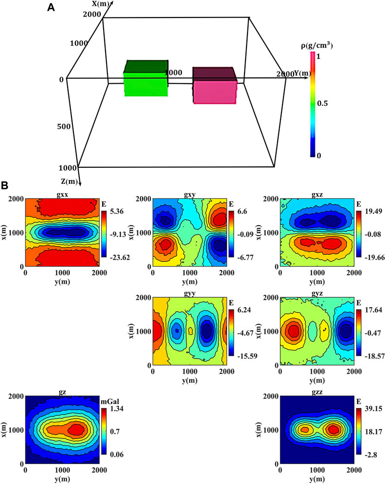
FIGURE 1. (A) The location of the two anomaly bodies. (B) Gravity and gravity gradient anomalies contaminated by 5% Gaussian random noise.

To quantitatively evaluate the inversion results, the relative root mean square (RMS) error s1 between the predicted anomalies by the inversion results in d_pred and the observed anomalies d_obs, and the RMS error s2 between the inverted density m_cal and the actual density m_real is calculated according to Eq. 23 (Wu, 2016) and Eq. 24, respectively

$s1=\frac{\sqrt{{\displaystyle {\sum }_{i=1}^N}{\left({\mathit{d}}_{\mathit{pred}}^i-{\mathit{d}}_{\mathit{obs}}^i\right)}^2}}{\sqrt{{\displaystyle {\sum }_{i=1}^N}{{\mathit{d}}_{\mathit{obs}}^i}^2}}(23)$

$s2=\sqrt{\frac{{\displaystyle {\sum }_{i=1}^M}{\left({\mathit{m}}_{\mathit{cal}}^i-{\mathit{m}}_{\mathit{real}}^i\right)}^2}{M}}(24)$

3.2 Comparison between inversion results of different algorithms

Three algorithms are used for the joint inversion and the results are compared. Algorithm 1 uses the conventional SL0 (the SL0 sparse recovery) from Meng (2016). Algorithm 2 constructs the objective function with L₂ norm based on the regularization theory. Algorithm 3 is the one proposed in this study, that is, SL0 regularization. The same weighting and constraint are applied to them.

Starting from a case of small-scale data, the subsurface domain is divided sparser than the default, into 20 × 20 × 10 prisms with the size of 100 × 100 × 100 m, the observation points also distribute on z = 0 plane and overlap the projection of prisms’ center of mass on the plane. Firstly, no noise is added to forward modeling. The inversion results are shown in Figure 2. Algorithm 3 (Figure 2C) has much less time cost t1 than Algorithm 1 (Figure 2A) and much better model fitting than Algorithm 2 (Figure 2B) which is the most obvious at z = 550 m plane and also reflected by the less RMS errors s1 and s2. These results indicate that compared with using the conventional SL0 in joint inversion, using SL0 regularization has successfully improved its efficiency while also preserving its advantage of high accuracy.

FIGURE 2

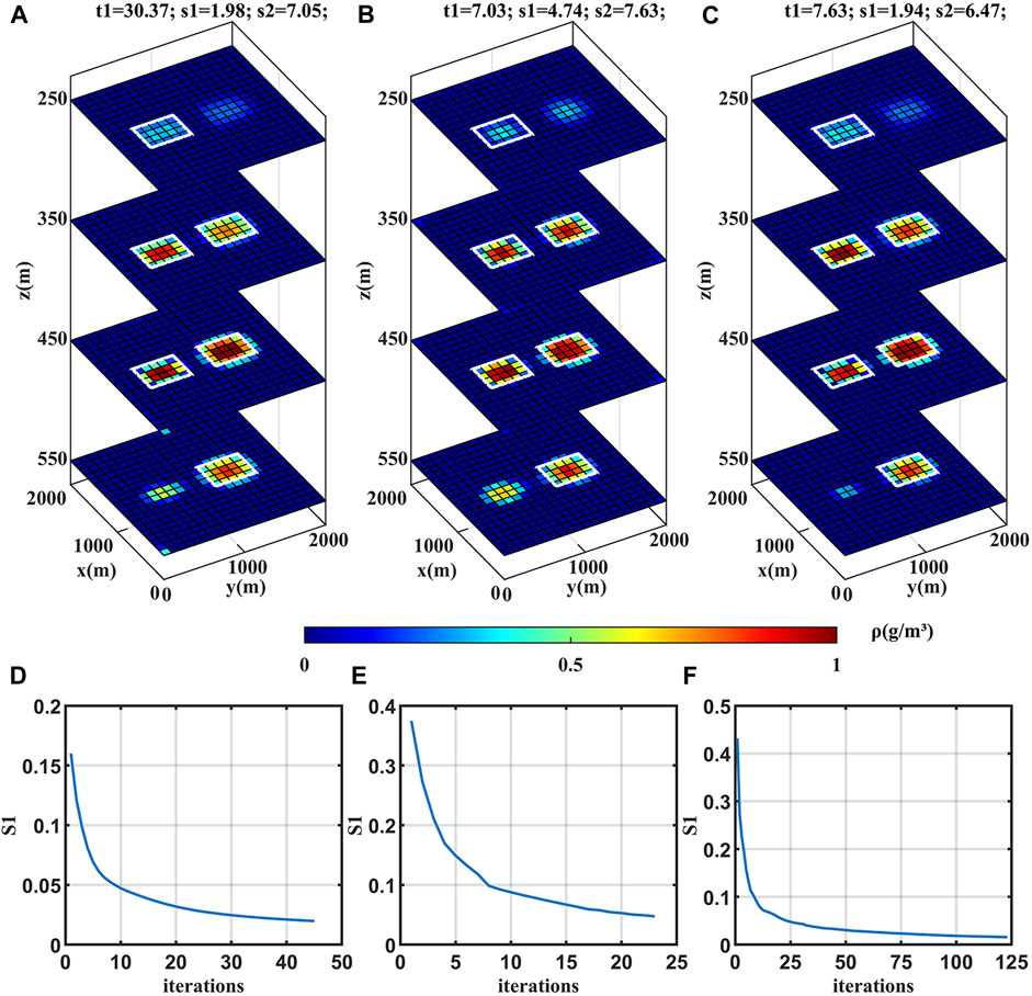
FIGURE 2. (A–C) Inversion results of Algorithms 1–3, respectively, using small-scale data without noise. The time cost t1 (s), RMS errors s1 (×0.01), and s2 (×0.01 g/cm³) are recorded on topside. The white solid lines mark the outlines of the anomaly bodies. (D–F) The variation of the relative RMS error s1 as a function of the total number of iterations for Algorithms 1–3, respectively.

Then 5% Gaussian random noise is added on the forward modeling of the above case to repeat the experiment. As shown in Figure 3, Algorithm 1 (Figure 3A) is very sensitive to noise; the major reason is that it overlays gravity and gravity gradient data in the calculation. In comparison, the behaviors of Algorithm 2 (Figure 3B) and Algorithm 3 (Figure 3C) are both similar to those without noise, which means that our algorithm has better anti-noise performance than the conventional SL0.

FIGURE 3

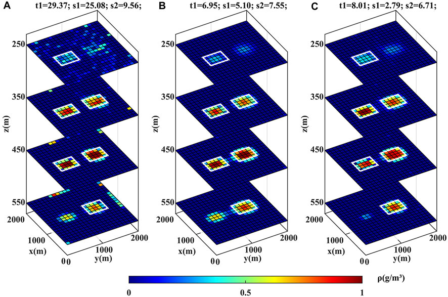
FIGURE 3. (A–C) Inversion results of Algorithms 1–3, respectively, using small-scale data with 5% Gaussian random noise.

Finally, the default division, that is, into 40 × 40 × 10 prisms, is applied in the case of large-scale data, and the inversion results are depicted in Figure 4. The t1 for Algorithm 3 (Figure 4C) is only 1/6 of that for Algorithm 1 (Figure 4A). That is to say, the improvement of our algorithm on efficiency, compared with the conventional SL0, is more obvious when inverting large-scale data. Additionally, compression of the sensitivity matrix is performed on Algorithm 3, then t1 is further shortened to 270.99 s, which confirms the effectiveness of this method.

FIGURE 4

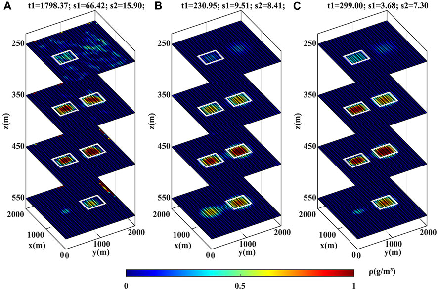
FIGURE 4. Similar to Figure 3 but using large-scale data.

3.3 The impacts of the data weighting matrix and the self-adaptive regularization parameter

To validate the data weighting matrix W_d, three methods are used in our algorithm separately. Method 1 is not using W_d, Method 2 is using the W_d according to Li et al. (2017), and Method 3 is using the W_d proposed in this study. Figure 5 displays the variation of s1 as a function of the total number of iterations when using these methods in the default experiment (denser division with 5% Gaussian random noise). Method 3 (Figure 5C) results in a closer fitting degree of different components and also a fewer number of iterations, which have confirmed the validity of the data weighting matrix in this study.

FIGURE 5

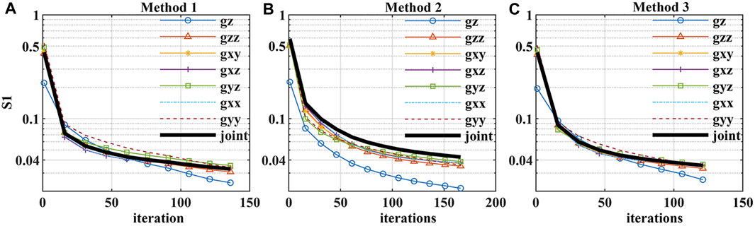
FIGURE 5. (A–C) The variation of the relative RMS error s1 of gravity or gravity gradient components and the combination of them, as a function of the total number of iterations for Methods 1–3, respectively.

To demonstrate the advantage of using the self-adaptive regularization parameter μ, another inversion is conducted using μ from the L-curve method, which is widely used for μ determination (Hansen, 1992). As shown in Figure 6, using the L-curve and the self-adaptive μ results in a similar fitting degree, but the latter needs much fewer iterations than the former, which means that using the self-adaptive μ could improve the convergence rate of the inversion.

FIGURE 6

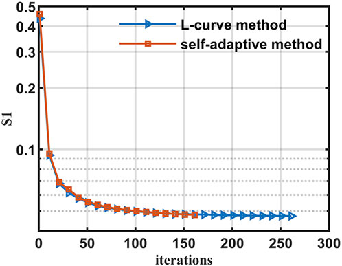
FIGURE 6. The variation of the relative RMS error s1 as a function of the total number of iterations when using the L-curve μ (blue line) and the self-adaptive μ (orange line).

3.4 The impacts of the model weighting, depth weighting, and density constraint

To demonstrate the effects of the model weighting and the depth weighting, another inversion is conducted only using the model weighting and the results are compared with those of the default inversion using both of them, as depicted in Figure 7. It is shown that only using the model weighting in the inversion could still reflect the horizontal locations of the anomaly bodies well (Figure 7A). In the vertical plane (Figure 7C), however, the inverted anomaly bodies have deeper depth and are more divergent than the actual ones. Adding the depth weighting function could obtain a more accurate and convergent result, as shown in Figure 7D. The above comparison suggests that when prior information is insufficient, it is feasible and reasonable to only use the model weighting in the inversion; otherwise, the depth weighting should be added to further optimize the results in the vertical direction.

FIGURE 7

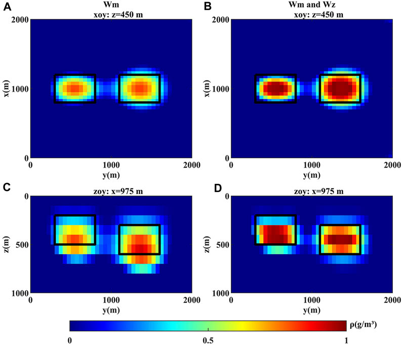
FIGURE 7. Inversion results of (A,C) only using the model weighting and (B,D) using both the depth and the model weighting. The black solid lines mark the outlines of the anomaly bodies.

To investigate our algorithm’s dependence on the range of the density constraint, another two constraints with a larger range of [0, 2] and a smaller range of [0, 0.5] are applied to the inversion separately; the results are compared with that using the accurate (default) range of [0, 1] and plotted in Figure 8. It is clearly shown that using an inaccurate density range could also roughly determine the locations of the anomaly bodies. A much smaller range would result in much lower inverted densities than the actual ones (see Figure 8B, E); by contrast, a much larger range has less impact (see Figure 8A, D). Therefore, it is better to choose a larger range for the density constraint when prior information is insufficient.

FIGURE 8

FIGURE 8. Inversion results under the density constraint of (A,D) [0, 2], (B,E) [0, 0.5], and (C,F) [0, 1] (default). The black solid lines mark the outlines of the anomaly bodies.

4 Application to real data

The real data used in this study were measured over the Vinton salt dome. The Vinton salt dome is located in southwestern Louisiana, United States. It consists of a core of massive salt and a well-defined cap rock which successively grades from limestone at the top to gypsum and anhydrite at the bottom (Coker et al., 2007). The density of the cap rock is 2.75 g/cm³ (Ennen, 2012).

Gravity data were measured on the ground, and airborne full tensor gravity gradient data were measured at an average altitude of 80 m. We select a subset of the area for investigation, which covers 3332550–3336450 m in x-direction (northwards) and 440550–444450 m in y-direction (eastwards) under the WGS84, UTM15N coordinate system. The z-axis is set vertically downwards. For the gravity data, a second-order polynomial fitting is applied to remove the regional field and obtain the residual anomaly at z = 0 m (Figure 9G). For the gravity gradient data, the terrain effect is removed with a density of 1.9 g/cm³ (Ennen, 2012), then a band-pass filtering of 200 − 5,000 m spatial wavelength (Geng et al., 2014) is used to obtain the residual anomalies for different components at z = −80 m (Figures 9A–F).

FIGURE 9

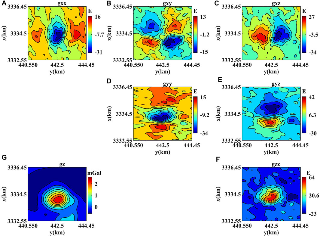
FIGURE 9. (G) Gravity residual anomaly at z = 0 m and (A–F) gravity gradient residual anomalies at z = −80 m, over the Vinton salt dome.

The inversion domain is divided into 40 × 40 × 20 prisms with the size of 100 × 100 × 50 m, so the depth range in this inversion is z = 0–1,000 m. The observation points of gravity (gravity gradient) anomaly distribute on z = 0 m (z = −80 m) plane and overlap the projections of prisms’ center of mass on the plane. The density structure is inverted using g_z, g_zz, g_xx|g_xy|g_xz|g_yy|g_yz|g_zz, the combination of g_z and g_xx|g_xy|g_xz|g_yy|g_yz|g_zz, separately. The minimum and maximum values of the density constraint are set to 0 g/cm³ and 0.6 g/cm³. The standard deviations (std) of the residuals between the observed gravity/gravity gradient data and the predicted ones by the inversion results are shown in Table 1. The inversion using g_z has the least std of gravity but a much larger std of gravity gradient than the other three cases. Using six components of gravity gradient (g_xx|g_xy|g_xz|g_yy|g_yz|g_zz) results in a lower std of gravity gradient than using g_zz. Additionally, the joint inversion of g_z and six components of gravity gradient further lowers the std, indicating that the joint inversion could obtain the most reasonable results.

TABLE 1

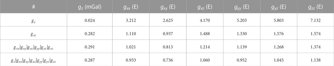
TABLE 1. The standard deviations of the residuals between the observed and predicted gravity/gravity gradient data for the four cases discussed.

Figure 10 displays the joint inversion results using g_z and g_xx|g_xy|g_xz|g_yy|g_yz|g_zz. In the horizontal plane, the length of the inverted anomaly body with high density is approximately 1,500 m in the east-west direction and 1,200 m in the north-south direction, consistent with the values of 1,520 m and 1,280 m from geological data (Ennen, 2012). It is wedge-shaped with a fracture in the northwestern direction, which has been revealed by the geological model obtained through drilling and seismic data (Coker et al., 2007). In the vertical plane, the fracture divides the topside of the anomaly body. The northwestern part has a deeper upper boundary of about 300 m and a thinner thickness of about 150 m; for the southeastern part, these two values are 250 m and 200 m. In comparison, drilling data (Thompson and Eichelberger, 1928) reveal that the depth of the upper boundary is 315 m in the north and 200 m in the south, and the average thickness is 150 m; geophysical inversion using gravity gradient data (Gao and Huang, 2017) reports that the depth of the upper boundary is 300 m in the northwest and 200 m in the southeast, and the average thickness is 250 m. The main features of our results are generally consistent with those of previous studies, which confirms the feasibility of our algorithm.

FIGURE 10

FIGURE 10. Joint inversion results over the Vinton salt dome using g_z and g_xx|g_xy|g_xz|g_yy|g_yz|g_zz. (A) Horizontal slices at different depths. (B) zoy slice at x = 3,334.3 km. (C) zox slice at y = 442.5 km.

5 Conclusion

In this study, we propose a new algorithm for joint inversion of gravity and gravity gradient data. The objective function is constructed using SL0 based on the regularization theory, then the optimal solution is derived with the non-linear conjugate gradient method. Additionally, a method of compressing the sensitivity matrix is also applied.

The numerical modeling shows that our algorithm is much more efficient than using the conventional SL0, especially when inverting large-scale data, and also has better anti-noise performance. On the other hand, our algorithm preserves the advantage of high accuracy, when compared with using L₂ norm as the objective function. Compression of the sensitivity matrices could further improve the efficiency of the inversion. Sensitivity analysis indicates that introducing the data weighting and self-adaptive regularization parameter has improved the convergence rate of the inversion. Additionally, it suggests using the model weighting and a larger range for the density constraint when prior information is insufficient; otherwise, the depth weighting should be added to further optimize the results in the vertical direction.

Finally, our algorithm is applied to the gravity and gravity gradient measurements at the Vinton salt dome. It is shown that the joint inversion using g_z and six components of gravity gradient g_xx|g_xy|g_xz|g_yy|g_yz|g_zz could obtain more reasonable results than using gravity or gravity gradient independently. The agreement of the inverted distribution range, thickness, and geometry of the cap rock with previous studies based on geological data, drilling data, seismic data, etc. has validated the feasibility of this algorithm in actual geological conditions.

Data availability statement

The original contributions presented in the study are included in the article/Supplementary material, further inquiries can be directed to the corresponding author.

Author contributions

TN: Writing–original draft. GaZ: Writing–review and editing. MZ: Writing–review and editing. GuZ: Writing–review and editing.

Funding

The authors declare financial support was received for the research, authorship, and/or publication of this article. This work was supported in part by the National Natural Science Foundation of China under Grant 41974060, and in part by the Stable-Support Scientific Project of the China Research Institute of Radiowave Propagation under Grant A132007W06.

Conflict of interest

The authors declare that the research was conducted in the absence of any commercial or financial relationships that could be construed as a potential conflict of interest.

Publisher’s note

All claims expressed in this article are solely those of the authors and do not necessarily represent those of their affiliated organizations, or those of the publisher, the editors and the reviewers. Any product that may be evaluated in this article, or claim that may be made by its manufacturer, is not guaranteed or endorsed by the publisher.

References

Beiki, M. (2010). Analytic signals of gravity gradient tensor and their application to estimate source location. Geophysics 75, I59–I74. doi:10.1190/1.3493639

CrossRef Full Text | Google Scholar

Bhatt, J. S., Joshi, M. V., and Raval, M. S. (2014). A data-driven stochastic approach for unmixing hyperspectral imagery. IEEE J. Sel. Top. Appl. Earth Observations Remote Sens. 7, 1936–1946. doi:10.1109/jstars.2014.2328597

CrossRef Full Text | Google Scholar

Capriotti, J., and Li, Y. (2014). “Gravity and gravity gradient data: understanding their information content through joint inversions,” in SEG international exposition and annual meeting (SEG). SEG–2014.

CrossRef Full Text | Google Scholar

Capriotti, J., and Li, Y. (2022). Joint inversion of gravity and gravity gradient data: a systematic evaluation. Geophysics 87, G29–G44. doi:10.1190/geo2020-0729.1

CrossRef Full Text | Google Scholar

Chen, Z.-X., Meng, X.-H., Guo, L.-H., and Liu, G.-F. (2012). Three-dimensional fast forward modeling and the inversion strategy for large scale gravity and gravimetry data based on gpu. Chin. J. Geophys. 55, 4069–4077. doi:10.6038/j.issn.0001-5733.2012.12.019

CrossRef Full Text | Google Scholar

Coker, M. O., Bhattacharya, J. P., and Marfurt, K. J. (2007). Fracture patterns within mudstones on the flanks of a salt dome: syneresis or slumping? Gulf Coast Assoc. Geol. Soc. Trans. 57, 125–137.

Google Scholar

Commer, M. (2011). Three-dimensional gravity modelling and focusing inversion using rectangular meshes. Geophys. Prospect. 59, 966–979. doi:10.1111/j.1365-2478.2011.00969.x

CrossRef Full Text | Google Scholar

Commer, M., Newman, G. A., Williams, K. H., and Hubbard, S. S. (2011). 3d induced-polarization data inversion for complex resistivity. Geophysics 76, F157–F171. doi:10.1190/1.3560156

CrossRef Full Text | Google Scholar

Dai, Y., and Yuan, Y. (1999). A non-linear conjugate gradient method with a strong global convergence property. SIAM J. Optim. 10, 177–182. doi:10.1137/S1052623497318992

CrossRef Full Text | Google Scholar

Ennen, C. (2012). Mapping gas-charged fault blocks around the vinton salt dome, Louisiana using gravity gradiometry data. Houston: Master thesis, University of Houston.

Google Scholar

Gao, X.-H., and Huang, D.-N. (2017). Research on 3d focusing inversion of gravity gradient tensor data based on a conjugate gradient algorithm. Chin. J. Geophys. 60, 1571–1583. doi:10.6038/cjg20170429

CrossRef Full Text | Google Scholar

Gebre, M. G., and Lewi, E. (2023). Gravity inversion method using l₀-norm constraint with auto-adaptive regularization and combined stopping criteria. Solid earth. 14, 101–117. doi:10.5194/se-14-101-2023

CrossRef Full Text | Google Scholar

Geng, M., Huang, D., Yang, Q., and Liu, Y. (2014). 3d inversion of airborne gravity-gradiometry data using cokriging. Geophysics 79, G37–G47. doi:10.1190/geo2013-0393.1

CrossRef Full Text | Google Scholar

Geng, M., Yang, Q., and Huang, D. (2017). 3d joint inversion of gravity-gradient and borehole gravity data. Explor. Geophys. 48, 151–165. doi:10.1071/eg15023

CrossRef Full Text | Google Scholar

Guo, Q., Ba, J., and Luo, C. (2020). Prestack seismic inversion with data-driven mrf-based regularization. IEEE Trans. Geoscience Remote Sens. 59, 7122–7136. doi:10.1109/tgrs.2020.3019715

CrossRef Full Text | Google Scholar

Guo, Q., Zhang, H., Han, F., and Shang, Z. (2017). Prestack seismic inversion based on anisotropic markov random field. IEEE Trans. Geoscience Remote Sens. 56, 1069–1079. doi:10.1109/tgrs.2017.2758800

CrossRef Full Text | Google Scholar

Hansen, P. C. (1992). Analysis of discrete ill-posed problems by means of the l-curve. SIAM Rev. 34, 561–580. doi:10.1137/1034115

CrossRef Full Text | Google Scholar

Jing, L., Yao, C.-L., Yang, Y.-B., Xu, M.-L., Zhang, G.-Z., and Ji, R.-Y. (2019). Optimization algorithm for rapid 3d gravity inversion. Appl. Geophys. 16, 507–518. doi:10.1007/s11770-019-0781-2

CrossRef Full Text | Google Scholar

Kowalski, M., and Torrésani, B. (2009). Sparsity and persistence: mixed norms provide simple signal models with dependent coefficients. Signal, image video Process. 3, 251–264. doi:10.1007/s11760-008-0076-1

CrossRef Full Text | Google Scholar

Lelievre, P. G., and Farquharson, C. G. (2013). Gradient and smoothness regularization operators for geophysical inversion on unstructured meshes. Geophys. J. Int. 195, 330–341. doi:10.1093/gji/ggt255

CrossRef Full Text | Google Scholar

Li, H., Fang, J., Wang, X., Liu, J., Cui, R., Chen, M., et al. (2017). Quantitative analysis of hepatic microcirculation in Rabbits After liver ischemia-reperfusion Injury Using Contrast-enhanced ultrasound. Chin. J. Geophys. 60, 2469–2476. doi:10.1016/j.ultrasmedbio.2017.06.004

PubMed Abstract | CrossRef Full Text | Google Scholar

Li, X., and Chouteau, M. (1998). Three-dimensional gravity modeling in all space. Surv. Geophys. 19, 339–368. doi:10.1023/a:1006554408567

CrossRef Full Text | Google Scholar

Li, Y., and Oldenburg, D. W. (1998). 3-d inversion of gravity data. Geophysics 63, 109–119. doi:10.1190/1.1444302

CrossRef Full Text | Google Scholar

Liu, S., Wan, X., Jin, S., Jia, B., Lou, Q., Xuan, S., et al. (2023). Joint inversion of gravity and vertical gradient data based on modified structural similarity index for the structural and petrophysical consistency constraint. Geodesy Geodyn. 14, 485–499. doi:10.1016/j.geog.2023.02.004

CrossRef Full Text | Google Scholar

Ma, G.-Q., Du, X.-J., and Li, L.-L. (2012). Interpretation of potential field tensor data using the tensor local wavenumber method and comparison with the conventional local wavenumber method. Chin. J. Geophys. 55, 380–393. doi:10.1002/cjg2.1733

CrossRef Full Text | Google Scholar

Meng, Z. (2016). 3d inversion of full gravity gradient tensor data using sl0 sparse recovery. J. Appl. Geophys. 127, 112–128. doi:10.1016/j.jappgeo.2016.02.010

CrossRef Full Text | Google Scholar

Mohimani, H., Babaie-Zadeh, M., and Jutten, C. (2009). A fast approach for overcomplete sparse decomposition based on smoothed l⁰ norm. IEEE Trans. Signal Process. 57, 289–301. doi:10.1109/tsp.2008.2007606

CrossRef Full Text | Google Scholar

Paoletti, V., Fedi, M., Italiano, F., Florio, G., and Ialongo, S. (2016). Inversion of gravity gradient tensor data: does it provide better resolution? Geophys. J. Int. 205, 192–202. doi:10.1093/gji/ggw003

CrossRef Full Text | Google Scholar

Pérez, D. O., Velis, D. R., and Sacchi, M. D. (2017). Three-term inversion of prestack seismic data using a weighted l2, 1 mixed norm. Geophys. Prospect. 65, 1477–1495. doi:10.1111/1365-2478.12500

CrossRef Full Text | Google Scholar

Portniaguine, O., and Zhdanov, M. S. (1999). Focusing geophysical inversion images. Geophysics 64, 874–887. doi:10.1190/1.1444596

CrossRef Full Text | Google Scholar

Qin, P., Huang, D., Yuan, Y., Geng, M., and Liu, J. (2016). Integrated gravity and gravity gradient 3d inversion using the non-linear conjugate gradient. J. Appl. Geophys. 126, 52–73. doi:10.1016/j.jappgeo.2016.01.013

CrossRef Full Text | Google Scholar

Qin, P.-B., and Huang, D.-N. (2016). Integrated gravity and gravity gradient data focusing inversion. Chin. J. Geophys. 59, 2203–2224. doi:10.6038/cjg20160624

CrossRef Full Text | Google Scholar

Rezaie, M. (2023). Focusing inversion of gravity data with an error function stabilizer. J. Appl. Geophys. 208, 104890. doi:10.1016/j.jappgeo.2022.104890

CrossRef Full Text | Google Scholar

Thompson, S. A., and Eichelberger, O. (1928). Vinton salt dome, calcasieu parish, Louisiana. AAPG Bull. 12, 385–394. doi:10.1306/3D9327EC-16B1-11D7-8645000102C1865D

CrossRef Full Text | Google Scholar

Tikhonov, A. N., and Arsenin, V. Y. (1977). Solutions of ill-posed problems.

Google Scholar

Tu, C., Liang, Q., Tao, C., Guo, Z., Hu, Z., and Chen, C. (2022). Gravity data reveal new evidence of an axial magma chamber beneath segment 27 in the southwest indian ridge. Minerals 12, 1221. doi:10.3390/min12101221

CrossRef Full Text | Google Scholar

Wang, N., Ma, G., Li, L., Wang, T., and Li, D. (2022). A density-weighted and cross-gradient constrained joint inversion method of gravity and vertical gravity gradient data in spherical coordinates and its application to lunar data. IEEE Trans. Geoscience Remote Sens. 60, 1–11. doi:10.1109/tgrs.2022.3196052

CrossRef Full Text | Google Scholar

Wang, T.-H., Huang, D.-N., Ma, G.-Q., Meng, Z.-H., and Li, Y. (2017). Improved preconditioned conjugate gradient algorithm and application in 3d inversion of gravity-gradiometry data. Appl. Geophys. 14, 301–313. doi:10.1007/s11770-017-0625-x

CrossRef Full Text | Google Scholar

Wu, L. (2016). Efficient modelling of gravity effects due to topographic masses using the Gauss–FFT method. Geophys. J. Int. 205, 160–178. doi:10.1093/gji/ggw010

CrossRef Full Text | Google Scholar

Wu, L., Ke, X., Hsu, H., Fang, J., Xiong, C., and Wang, Y. (2012). Joint gravity and gravity gradient inversion for subsurface object detection. IEEE Geoscience Remote Sens. Lett. 10, 865–869. doi:10.1109/LGRS.2012.2226427

CrossRef Full Text | Google Scholar

Yao, C., Hao, T., Guan, Z., and Zhang, Y. (2003). High-speed computation and efficient storage in 3-d gravity and magnetic inversion based on genetic algorithms. Chin. J. Geophys. 46, 252–258.

CrossRef Full Text | Google Scholar

Yin, X., Yao, C., Zheng, Y., Xu, W., Chen, G., and Yuan, X. (2023). A fast 3d gravity forward algorithm based on circular convolution. Comput. Geosciences 172, 105309. doi:10.1016/j.cageo.2023.105309

CrossRef Full Text | Google Scholar

Zhang, C., Mushayandebvu, M. F., Reid, A. B., Fairhead, J. D., and Odegard, M. E. (2000). Euler deconvolution of gravity tensor gradient data. Geophysics 65, 512–520. doi:10.1190/1.1444745

CrossRef Full Text | Google Scholar

Zhang, R., Li, T., Liu, C., Li, F., Deng, X., and Shi, H. (2021). Three-dimensional joint inversion of gravity and gravity gradient data based on data space and sparse constraints. Chin. J. Geophys. 64, 1074–1089.

Google Scholar

Zhao, G., Wang, X., Liu, J., Chen, B., Kaban, M. K., and Xu, Z. (2023). 3d gravity inversion based on mixed-norm regularization in spherical coordinates with application to the lunar moscoviense basin. Geophysics 88, G67–G78. doi:10.1190/geo2022-0285.1

CrossRef Full Text | Google Scholar

Zhao, S., Gao, X., Qiao, Z., Jiang, D., Zhou, F., and Lin, S. (2018). 3d joint inversion of gravity and gravity tensor data. Glob. Geol. 21, 55–61. doi:10.3969/j.issn.1673-9736.2018.01.06

CrossRef Full Text | Google Scholar

Zhdanov, M. S. (2002). Geophysical inverse theory and regularization problems, 36. Elsevier.

Google Scholar

Zhdanov, M. S. (2009). New advances in regularized inversion of gravity and electromagnetic data. Geophys. Prospect. 57, 463–478. doi:10.1111/j.1365-2478.2008.00763.x

CrossRef Full Text | Google Scholar