 Wanjin Zhao
 Weitao Sun
 Jianhu Gao1
 Run He
94% of researchers rate our articles as excellent or good
Learn more about the work of our research integrity team to safeguard the quality of each article we publish.
Find out more
ORIGINAL RESEARCH article
Front. Earth Sci., 29 December 2023
Sec. Solid Earth Geophysics
Volume 11 - 2023 | https://doi.org/10.3389/feart.2023.1269616
This article is part of the Research TopicAdvances of New Technologies in Seismic ExplorationView all 22 articles
The wave characteristics of fractured-porous media can be utilized for permeability identification; however, further research is necessary to enhance the accuracy of this identification. A novel wave equation for fractured-porous media is formulated, and theoretical analysis suggests its effectiveness in accurately identifying reservoir permeability. The proposed methodology establishes a wave equation for fractured-porous media using the volume averaging method and employs finite difference method on staggered grids to calculate wave field dispersion and attenuation, exploring the influence of fracture network structure and confining pressure on the solution of the wave equation. By analyzing the wave equation under various aspect ratios and confining pressure of fractures, it is observed that these factors significantly affect velocity and attenuation, providing valuable insights into seismic response in fractured-porous media. Furthermore, the research findings reveal promising potential in utilizing the new wave equations specific to fractured-porous media for permeability identification purposes. By constructing a three-dimensional fractured-porous network model, the wave equation for permeability identification can examine the correlation between the parameters of the equation and permeability, and establishes an association between fracture parameters and permeability, paving the way for a novel approach to permeability identification.
The permeability is one of the crucial parameters for evaluating reservoir storage performance. Previous research has demonstrated that analyzing wave behavior in fractured-porous media can improve the accuracy of identifying reservoir permeability. The prediction of reservoir permeability using the wave equation in fractured-porous media can be categorized into three distinct stages. In the initial stage, Biot (1956a, b), based on the homogeneous porous media model and discovered that variations in permeability can lead to frequency dispersion and attenuation of seismic wave, resulting in changes in seismic velocity, which provided the foundation for subsequent related studies. In the subsequent stage, Numerous fractured-porous media models (Schoenberg, 1980; Schoenberg, 1983; Schoenberg and Douma, 1988; Schoenberg and Sayers, 1995; Gurevich et al., 2009; Tang, 2011; Tang et al., 2012) on Biot’s theory have been developed to investigate the relationship between permeability and seismic velocity in fractured-porous media. For instance, Chapman (Chapman et al., 2002; Chapman et al., 2016) established a microscale porous model, yet failed to provide an expression for the permeability of the porous media. Chichinina (Chichinina et al., 2007; Chichinina et al., 2009) proposed an anisotropic model for horizontally layered fractures that focused on P/S wave attenuation but did not address the permeability in fracture system. Gurevich (Gurevich et al., 2009), using a constructed fractured-porous media model, observed significant variations in velocity due to changes in the structures of pore and fracture, while changes in permeability resulted in relatively minor alterations in wavefield velocity. However, these studies did not explicitly explore the relationship between velocity and microstructure or permeability of fractured-porous media due to limitations in computer technology at that time. In the third stage, researchers initiated the construction of fractured-porous models incorporating microstructure, studying the relationship between fractures and wavefield velocity as well as reservoir permeability. For example, Du et al. (2011) studied an equivalent media model for fractured porous rocks. Fractures are modeled by constitutive relationship in terms of fracture-induced anisotropy. Guo et al. (2018) used the branch function method to construct finite-thickness fractures and examined the dispersion and attenuation of P-wave propagation perpendicular to the fracture surface. Lissa et al. (2019) explored the impact of fractures with varying widths on seismic attenuation and velocity dispersion. Song et al. (2020) investigated dispersion and attenuation of P-wave in heterogenous porous media containing oriented fractures, revealing that factors such as mechanical form of fractures and fluid flow properties significantly influence attenuation sensitivity. Wei et al. (2021) conducted research on a 3D fractured-porous network model, presenting a calculation approach for permeability while uncovering notable influences of aspect ratio on P-wave velocity and characteristic frequency. Wang et al. (2022) studied the propagation law for complex fractures in two-phase media through linear slip theory.
The prediction of reservoir permeability in fractured-porous media using the wave equation still encounters numerous challenges and difficulties. Firstly, it is imperative to enhance the microstructure and multiscale characteristics of fractured-porous media (Bai et al., 2021). Secondly, it is crucial to investigate the influences of factors such as fractures, confining pressure, permeability, and porosity on velocity as well as explore their interactions in fractured-porous media. Only through these efforts can we elucidate the relationship between wave properties and permeability in fractured-porous media.
The present work proposes a novel fractured-porous model and derives its wave equation based on volume averaging method, investigating the influence of fracture network structure on the solution of the wave equation and the relationship between fracture aspect ratio and wave velocity as well as permeability. This research possesses several distinctive features compared to previous studies: firstly, the solutions of the wave equation under different fracture aspect ratios and confining pressure conditions are studied; secondly, by analyzing various parameter combinations, such as velocity and attenuation, significant effects of fracture aspect ratio and confining pressure on wave behavior are revealed; thirdly, a proposed permeability identification method based on the curves of velocity-fracture parameters and velocity-permeability establishes correlations between fracture parameters and permeability.
Fractures exhibit a predominant extension direction, thus the elliptic cylindrical model can be used to describe their extensibility. The aspect ratio, defined as the ratio between the short and long radii of the elliptical cylinder cross-section, governs the structure of this model. As the aspect ratio approaches unity, it degenerates into a conventional porous model; whereas for very small values of aspect ratio, it accentuates more features of fracture structures. This flexible elliptical cylinder model enables us to depict various characteristics of fractures in reservoirs under different aspect ratios and provides insights into fracture structures with varying extensibility.
The derivation of the fluid motion equations in elliptic cylindrical fracture structure is presented below. The incompressible Newtonian fluid within the microtubule space of the elliptical cylinder satisfies the following equations (Landau and Lifshitz, 1987).
The equation of fluid mass conservation:
The equation of fluid momentum conservation:
Constitutive relationship of fluid mechanics:
where
The fluid velocity field is expressed as the combination of steady-state and unsteady-state fields:
Under low-speed flow conditions, the compressibility of pore fluid can be neglected when subjected to elastic waves (denoted as
The fluid dynamics equations mentioned above can be solved by the series expansion of Mathieu function in the elliptic cylindrical coordinate system, thereby obtaining the velocity field and flow rate in elliptic cylindrical space (Xiong et al., 2021). The expression for the steady-state flow rate at both ends of the elliptical cylinder is:
The expression describing the flow rate of the pulsating flow field is as follows:
The flow rate of the elliptic cylindrical fractures is observed to be dependent on various factors, including the length
The elliptical curve representation is inadequate for accurately depicting the tip of a genuine fracture. In order to precisely depict the variation in the major axis direction radius
Confining pressure signifies the force exerted by overlying geological materials on a specific point within the Earth’s crust. This pressure significantly affects permeability and elasticity of porous media. Firstly, under elevated confining pressure, the closure of pores and fractures within porous media leads to a significant reduction in permeability, diminishing the capacity for fluid flow. Secondly, confining pressure alters the elasticity of the porous material, specifically impacting its bulk modulus. This shift in elasticity has ramifications for the mechanical behavior of the material and the propagation of stress-related phenomena, including seismic waves.
In this study, it is assumed that flow conservation holds for each node in the fractured-porous network, ensuring that inflow equals outflow at every node. A flow conservation equation is formulated for each node, resulting in a system of linear equations with unknown variables representing the pressures at individual nodes. The pressures at the inlet and outlet are considered as non-homogeneous terms. By solving this system of equations to determine the pressures at each node, the flow within the 3D porous network can be accurately calculated. Furthermore, by incorporating Darcy’s law, dynamic permeability prediction for the 3D microtubule network in porous media can be effectively conducted (Xiong et al., 2021).
The volume averaging theorem, established by researchers like Whitaker (Whitaker, 1966; Whitaker, 1967), Slattery (1967), and Gray and Lee (1977), plays a pivotal role in connecting microscale parameters to macroscale behaviors within porous media. It has been widely applied in fields ranging from hydrogeology to geophysics, providing a consistent framework for modeling complex porous media systems. This theorem’s mathematical rigor and practical relevance have been extensively validated through real-world applications, underlining its significance. The use of the volume averaging theorem is firmly grounded in this well-established foundation of literature and research, reinforcing its vital role in this work and aligning with the reviewer’s emphasis on its importance. By introducing the volume average theorem, a connection between the macroscopic behavior of fractured-porous media and the microscopic parameters of the media is established, which derives a macroscopic wave equation that describes the wave behavior based on this theorem.
The unit cell region
Here, the micro characteristic length
The volume of the unit cell
where
According to the above definition, there is
According to the research conducted by Slattery (Slattery, 1967) and Whitaker (Whitaker, 1966) on the volume average theorem, considering the physical variable
The volume average term including time derivative is as follows:
where
Assuming the skeleton is initially static and satisfies the assumptions of linear elasticity and isotropy, its equation of microscale momentum conservation can be expressed as follows.
where
The microscopic constitutive equation of solid is:
where
The previous sections present the mass conservation equation, the momentum conservation equation and the constitutive equation of fluid. The equation of fluid state is expressed in the following form:
where
Assuming the presence of a porous media comprising a solid skeleton and a fluid, with only one existing interface denoted as
where
Based on the volume integral theorem, the macroscopic equation can be obtained by averaging the microscopic momentum conservation equation for fluids over the entire volume:
where
The stress
where
where
The equivalent bulk modulus of the porous unit with
where
Assuming that the shear stress in the porous media is solely borne by the solid skeleton, disregarding any fluid-induced shear deformation:
Where
In conclusion, the constitutive relationship between solid and fluid can be summarized as follows:
The final form of the wave equation is derived by combining the constitutive equation with the volume-averaged momentum conservation equation:
where,
The system of equations above represents the wave propagation control equation for porous media saturated with single fluid at low frequencies, wherein the unknowns are the displacements of solid and fluid particles denoted as
By applying the divergence operator to both sides of the wave Eq. 32 and introducing
By applying the curl operator to both sides of the wave Eq. 32 and introducing
The propagation of elastic waves in isotropic porous media is characterized by uniformity in all directions. Let the solution of the wave equation be expressed in the following prescribed form:
where
The system of equations will have non-zero solutions only if the determinant of the coefficient matrix is equal to zero, resulting in the dispersion equation:
where
where the coefficients
where
In general, for a given frequency
According to the method of plane wave analysis, the plane harmonic S-wave propagating along the
where
The system of equations will have non-zero solutions only if the determinant of the coefficient matrix is equal to zero, resulting in the dispersion equation:
where
In general, for a given frequency
Firstly, the wave equation in terms of displacement is transformed into the velocity-stress formulation. Subsequently, finite difference scheme is implemented on the staggered grid. Finally, by considering seismic source and boundary conditions, snapshots of wave field in porous media with non-uniform saturation distribution are computed.
By using
In the equation provided above, the brackets in
Here
It should be noted that the stress tensor exhibits symmetry, resulting in a total of 9 unknowns, namely,
The wave equation is represented in its component form by a set of 6 equations, while the constitutive equation is expressed through 7 equations, resulting in a total of 13 equations that correspond to the number of unknowns. It is assumed that both stress and velocity are initialized as zero at t=0. In the Cartesian coordinates, set
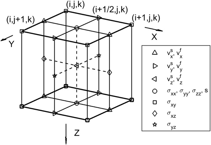
FIGURE 1. The schematic diagram of finite difference staggered grid.
The staggered grid differencing operators, denoted as
Here, the notation
Utilizing the staggered-grid finite difference, the discretization of unknown variables in the first-order velocity-stress equation occurs at distinct grid points, leading to the subsequent finite difference equations for velocity update:
The finite difference equations for stress update are as follows:
where
The selection of spatial step size should be based on the dispersion curve in order to determine the propagation velocity of seismic waves at a specific frequency. By calculating different types of wavelengths given the frequency, it is necessary to have at least 2–4 spatial grids within each wavelength, thus determining the appropriate spatial step size. The time step size should be determined by starting from the stability condition of the difference scheme and selecting a relatively small value to ensure that an unstable solution does not occur.
The seismic source is applied to the principal stresses
where
where
where
Taking the left boundary as an example,
Given the initial conditions, the wavefield’s physical variables at each node are known at time
where each coefficient refers to as follows:
Therefore, the calculation of the wavefield value at the node
The proposed method can be employed to implement absorbing boundary processing for other physical variables on boundaries within the wavefield region. Due to the directional nature of wave velocity on different boundaries, the wave velocity
To validate the effectiveness of the finite difference method for the wave equation in fractured-porous network, the core sample saturated oil shown in Table 1 is selected. Based on the finite difference in the staggered grid, the numerical solutions of the wave equation is obtained to generate wavefield snapshots, followed by the analysis of wavefield velocity and attenuation.
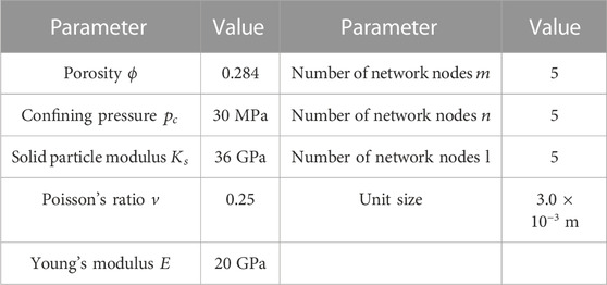
TABLE 1. Parameter table of porous media.
The parameters of the differential grid are presented in Table 2.
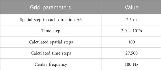
TABLE 2. Parameter table of finite difference simulation.
The calculation space range is

FIGURE 2. The wave field snapshot of oil-bearing fractured-porous media (The velocity of solid particle).
Wavefield information is computed using parameters corresponding to various aspect ratios, and the obtained results are compared with the dispersion and attenuation outcomes derived from plane wave analysis. The aspect ratio “a” ranges from 0.1 to 1.0 in increments of 0.1, resulting in a total of 10 values. In this study, the proposed method is employed to calculate the dry skeleton modulus and permeability (under steady flow conditions), which are subsequently substituted into both the numerical solution of the wave equation and the analytical solution of the plane wave analysis. The values of dry skeleton modulus and permeability for different aspect ratios are shown in Figure 3.
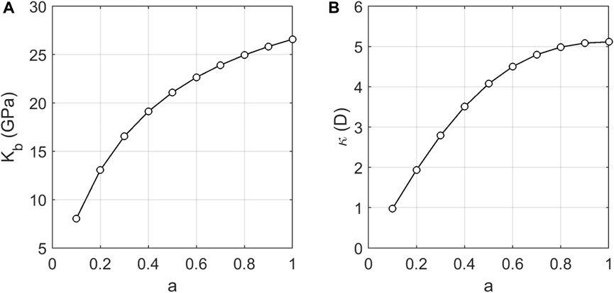
FIGURE 3. Dry skeleton modulus (Kb) and permeability (κ) corresponding to different aspect ratios (a).
The procedure for computing the dispersion and attenuation of fast P-wave based on seismic data is outlined as follows: Firstly, in the calculation process of the wave field snapshot, two receivers are strategically positioned to measure particle velocity and stress amplitude at distinct locations. Let
The theoretical solutions of dispersion and attenuation, along with the numerical results obtained from the finite difference method, are compared in Figures 4, 5. It can be observed from these figures that the fast P-wave velocity calculated using the proposed finite difference scheme exhibits excellent agreement with the theoretical solution based on plane wave analysis. Additionally, a consistent trend is observed for the inverse quality factor. These computational findings provide validation for the efficacy of the proposed method.
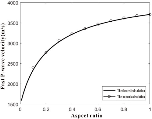
FIGURE 4. Comparison between theoretical solution and numerical solution of fast P-wave velocity under different aspect ratios.
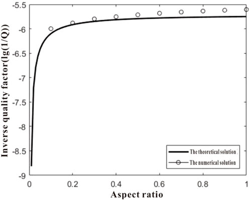
FIGURE 5. Comparison between theoretical solution and numerical solution of fast P-wave attenuation under different aspect ratios.
The confining pressure exerted on the porous media has a direct impact on
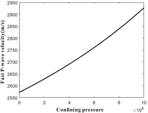
FIGURE 6. Variation of fast P wave velocity with confining pressure.
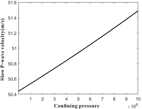
FIGURE 7. Variation of slow P wave velocity with confining pressure.
The calculation results demonstrate that the wave velocity increases with the applied confining pressure, owing to the concurrent rise in dry skeleton modulus
Based on this case study, it can be inferred that the velocities of fast P-waves and slow P-waves exhibit a gradual increase as the confining pressure increases. This observed trend remains consistent across different frequencies of seismic waves, particularly at relatively low frequencies (<104 Hz).
The propagation of waves in porous media containing fluids gives rise to phenomena such as dispersion and attenuation, wherein both the wave velocity and amplitude exhibit frequency-dependent changes. The dispersion and attenuation curves of the wavefield are influenced by rock physical properties including porosity, permeability, fluid properties, and solid skeleton bulk modulus. Among these factors, we specifically investigated the sensitivity of dispersion and attenuation curves to variations in permeability. If alterations in permeability can be discerned on dispersion/attenuation curves, it becomes feasible to estimate these changes through observation and calculation of these curves or even determination of numerical values for permeability using a template method.
According to the wave equation and plane wave analysis, expressions for dispersion/attenuation of the wave field has been yielded. The dispersion and attenuation curves of the wave field are then calculated based on rock physics parameters under different permeability. A set of solid skeleton parameters and fluid parameters is selected as presented in Table 3 (Johnson, 2001; Lo, et al., 2005).
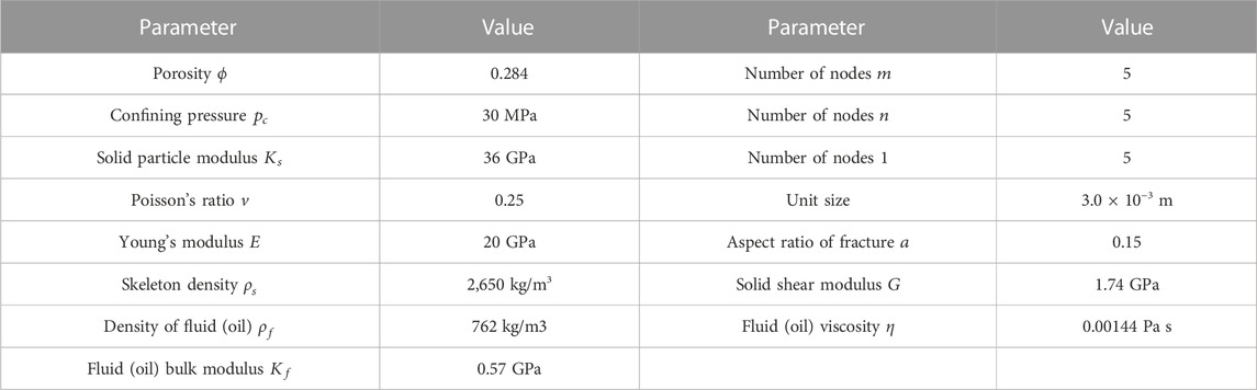
TABLE 3. Rock physical parameters.
The calculated dispersion/attenuation curves are depicted in Figures 8, 9.

FIGURE 8. Variation of fast P-wave dispersion curves with permeability.
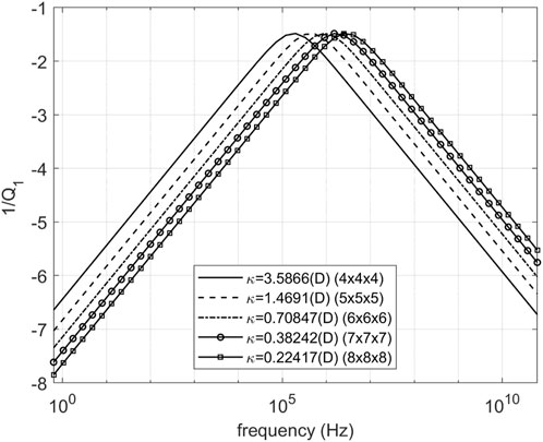
FIGURE 9. Variation of fast P-wave attenuation curves with permeability.
In the example, various porous network structures of different scales (
In conclusion, the permeability can be modified by adjusting the porous network structure (pore density), based on rock physical parameters such as porosity, fluid parameters, and solid skeleton bulk modulus. Different permeability conditions result in noticeable and regular changes in the wavefield curves of dispersion and attenuation. Therefore, it is possible to calculate the variation pattern of dispersion and attenuation with respect to permeability when rock physical parameters are known. Consequently, changes in permeability can be inferred by measuring the movement of dispersion/attenuation curves.
By utilizing the curves of permeability and bulk modulus for different fracture aspect ratios within a fully saturated elastic model, dispersion curves for P- and S-wave velocities, along with prediction for attenuation, are successfully derived. Subsequently, by obtaining the permeability and P/S-wave velocities in porous media with varying fracture aspect ratios, the plot can be drawn, illustrating the relationship between P/S-wave velocity and permeability.
The graphical analysis of seismic attributes is presented in Figure 10, illustrating the calculation results. For sandstone, the calculated parameters are as follows: density of 2,650 kg/m3, bulk modulus of 37 GPa, shear modulus of 44 GPa, Poisson’s ratio of 0.08, and Young’s modulus of 94.5 GPa. When determining wave velocity, a fixed frequency of 30 Hz is employed.
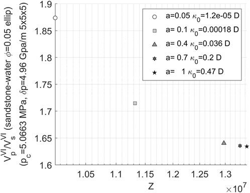
FIGURE 10. Relationship between P-wave velocity and permeability of 3D water-bearing fracture network.
The permeability gradually decreases as the aspect ratio of fractures decreases under a given porosity condition, as observed from Figure 10. The data points on the graph move from bottom right to top left, and with approaching zero aspect ratio, there is a rapid increase in the distance between data points.
From the calculation results, it is evident that there exists a significant variation in the velocity ratio of P- and S-wave under different fracture/pore aspect ratios, indicating a substantial impact of aspect ratio on this velocity ratio. The influence of aspect ratio on the velocity ratio arises from two aspects: 1) the effect of varying aspect ratios on the bulk modulus of rock skeleton; 2) the effect of varying aspect ratios on permeability. These two influences are closely intertwined, and when assessing the feasibility of predicting permeability using seismic attributes, both aspects need to be simultaneously considered rather than isolating one-sided effects.
As aspect ratio have effects on both bulk modulus and permeability, their contributions to the velocity ratio are intertwined, making it impossible to separately examine the influence of permeability on wave velocity. To further analyze the relationship between wave velocity ratio and permeability, the fracture aspect ratio parameter is held constant while varying only the numerical value of permeability, then calculate data for the velocity ratio-impedance template.
To facilitate comparison with previous examples, the aspect ratio is standardized to 1 and the corresponding permeability values from those examples (1.2
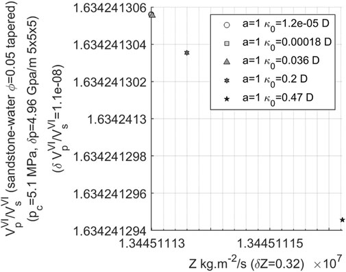
FIGURE 11. Variation of velocity ratio with impedance in 3D water-bearing fracture network.
From Figure 11, it is evident that when the aspect ratio remains constant (in this case, 1) and only the permeability varies, there is a significant reduction in the range of variation observed in the velocity ratio. Simultaneously, there is also a substantial decrease in the range of impedance changes. Within the same range of permeability variations as considered in previous calculations, discerning changes in permeability solely from the velocity ratio becomes nearly impossible. Hence, it can be concluded that alterations in bulk modulus resulting from variations in aspect ratio are primarily responsible for considerable changes observed in velocity ratio, while modifications in permeability due to changes in aspect ratio have relatively minor impacts on velocity ratio.
In order to ascertain the extent of permeability changes that can be discerned in the velocity ratio-impedance template, the variation pattern of velocity ratio as permeability ranged from 1 millidarcy to 100 darcies has been investigated. Figure 12 illustrates that when permeability exhibits a wide range of variability (0.001–100 Darcy), there is a significant amplification in the magnitude of impedance (from 0.32 to 130,000 kg/s.m2). Hence, during substantial fluctuations in permeability, corresponding variations in impedance become more pronounced. However, it should be noted that the numerical value for velocity ratio change remains exceedingly small (0.00041), rendering it inadequate for independently distinguishing alterations in permeability.
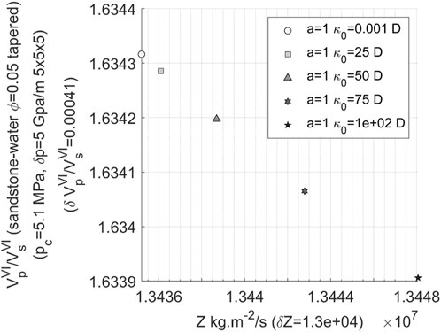
FIGURE 12. Variation of velocity ratio with impedance in 3D water-bearing fracture network (the permeability changing from 0.001 to 100 Darcy and the aspect ratio of 1).
The following analysis investigates the patterns observed under different aspect ratios, replicating the aforementioned calculations for aspect ratios of 0.5 and 0.05. Figures 13, 14 demonstrate that as the aspect ratio decreases, there is a significant reduction in the range of variation in wave impedance, decreasing from 130,000 kg/s.m2 at
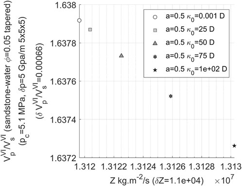
FIGURE 13. Variation of velocity ratio with impedance in 3D water-bearing fracture network (the permeability changing from 0.001 to 100 Darcy and the aspect ratio of 0.5).
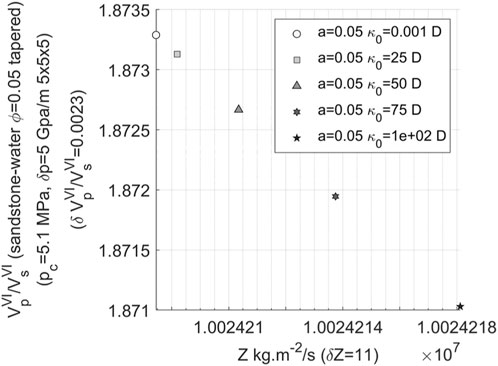
FIGURE 14. Variation of velocity ratio with impedance in 3D water-bearing fracture network (the permeability changing from 0.001 to 100 Darcy and the aspect ratio of 0.05).
From the analysis of the calculation results above, it is evident that when considering rocks with identical physical parameters and varying only in permeability, there is minimal variations observed in the velocity ratio of P- to S-wave at the frequency of 30 Hz. Consequently, identifying changes in permeability becomes exceedingly challenging. In scenarios where there exists a significant alteration in permeability (e.g., from 1 millidarcy to 100 Darcy), porous networks with the large aspect ratio exhibit a relatively extensive range of impedance variation. However, even within low porosity and low permeability rocks, the dispersion degree of data points on the velocity ratio-impedance template remains insufficient for isolating the impact of permeability changes, thereby presenting substantial challenges.
The variation patterns of P-wave attenuation and Young’s modulus in relation to different permeability have been carried out, revealing a significant range of relative changes in attenuation. Figure 15 illustrates the variations in P-wave attenuation-Young’s modulus resulting from alterations in permeability within water-bearing porous sandstone.
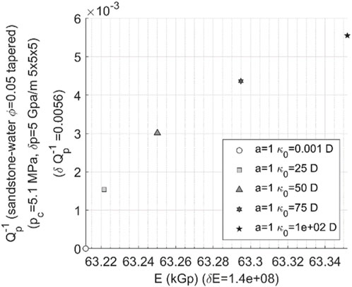
FIGURE 15. Template of P-wave velocity attenuation-Young’s modulus in 3D water-bearing fracture network (The permeability changing from 0.001 to 100 Darcy and the aspect ratio of 1.
The following conclusions can be inferred from the attenuation-Young’s modulus template:
(1) The relative change in P-wave attenuation is quite noticeable. As the permeability increases, the attenuation value gradually increases, exhibiting an approximately linear growth trend.
(2) With the increase in permeability, Young’s modulus also gradually increases, and it grows more rapidly at higher permeability.
(3) If accurate data on P-wave attenuation can be obtained, the velocity attenuation-Young’s modulus template can be utilized to analyze and identify changes in permeability within reservoir when permeability changes significantly in a wide range.
(4) In cases of low porosity and low permeability where there is limited variation in permeability, the distribution range of data points on the velocity attenuation-Young’s modulus template is also narrow, posing challenges for identifying changes in permeability.
In order to identify seismic attributes that exhibit high sensitivity to variations in permeability, the comprehensive sensitivity analysis on various seismic attribute parameters has been conducted. During the calculations, five permeability values were uniformly selected ranging from 0.001 Darcy to 100 Darcy, while keeping other rock physics parameters constant. The individual sensitivities of the velocity ratio of P- to S-wave, P-wave impedance, wave velocity, shear modulus, Young’s modulus, and attenuation of P- and S-wave velocities towards changes in permeability were separately evaluated. The parameters investigated in our study have distinct physical meanings in the context of fractured-porous media. The velocity ratio of P- to S-wave (Vp/Vs) serves as an indicator of fluid-filled zone. P-wave impedance (Z) and wave velocities (Vp and Vs) provide insights into rock density and elastic properties. Shear modulus (μ) and Young’s modulus (E) are mechanical properties that describe rock resistance to deformation, with lower values indicating increased deformability under stress. Lastly, attenuation parameters (Qp and Qs) quantify the energy loss of seismic waves, with higher permeability associated with greater attenuation, crucial for detecting fluid-saturated zones. These parameters collectively help in characterizing subsurface formations, fluid dynamics, and rock behavior in fractured-porous media, aiding in hydrocarbon exploration and reservoir assessment.
Herein, the sensitivity
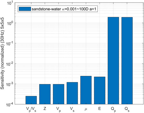
FIGURE 16. Sensitivity comparison of seismic attributes changing with permeability in 3D water-bearing fracture network (The permeability changing from 0.001 to 100 Darcy, the aspect ratio of 1 and the frequency of 30 Hz).
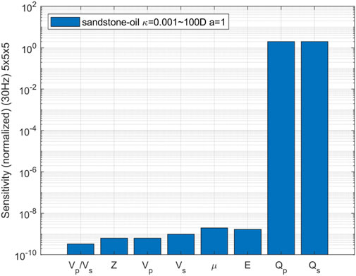
FIGURE 17. Sensitivity comparison of seismic attributes changing with permeability in 3D oil-bearing fracture network (The permeability changing from 0.001 to 100 Darcy, the aspect ratio of 1 and the frequency of 30 Hz).
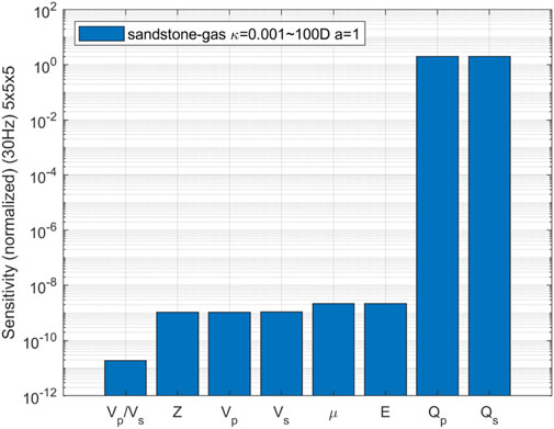
FIGURE 18. Sensitivity comparison of seismic attributes changing with permeability in 3D gas-bearing fracture network (The permeability changing from 0.001 to 100 Darcy, the aspect ratio of 1 and the frequency of 30 Hz).
The comparative analysis reveals that the sensitivity of seismic attributes, such as velocity ratio, P-wave impedance, wave velocity, shear modulus, and Young’s modulus, to changes in permeability is relatively low. Conversely, the attenuation of P-wave and S-wave velocities exhibits a comparatively high sensitivity. The additional calculation and analysis for the aspect ratio of 0.5 are conducted, finding that the sensitivity of seismic attributes to changes in permeability remains consistent with the case where the aspect ratio is 1.
In this paper, an improved wave equation of fractured-porous media is proposed. Through this research, the significant influence of fracture aspect ratio and confining pressure on wave properties is unveiled, and a novel method for permeability identification based on the curves of velocity-fracture parameters and velocity-permeability is proposed, while numerical simulation methods are refined. The research findings demonstrate that fracture aspect ratio and confining pressure exert a substantial impact on wave properties such as velocity and attenuation; there exists a correlation between fracture parameters and permeability, which can be utilized to predict permeability by utilizing the curves of either velocity-fracture parameters or velocity-permeability. These discoveries offer fresh insights into the wave behavior of fractured-porous media, providing a theoretical foundation and innovative approaches for permeability prediction. Moreover, the methodologies and concepts presented in this study can also be applied to seismic rock physics research in various fields, thereby further advancing related areas’ development. Nevertheless, certain limitations persist in this study including the complexity of fluid flow within porous media as well as challenges associated with accurately describing the actual motion state of pore fluid. In future research, these challenges will continue to be addressed to enhance models and methods, enhancing accuracy and applicability in permeability identification.
The original contributions presented in the study are included in the article/Supplementary Material, further inquiries can be directed to the corresponding author.
WZ: Data curation, Funding acquisition, Investigation, Writing–original draft. WS: Conceptualization, Formal Analysis, Methodology, Writing–original draft. JG: Project administration, Supervision, Validation, Writing–review and editing. RH: Investigation, Visualization, Writing–review and editing.
The authors declare financial support was received for the research, authorship, and/or publication of this article. This work was supported by the National Natural Science Foundation of China (Grant Nos 42074144 and 41874137).
Authors WZ, JG, and RH were employed by PetroChina.
The remaining author declares that the research was conducted in the absence of any commercial or financial relationships that could be construed as a potential conflict of interest.
The authors declare that this study received funding from CNPC Science Research and Technology Development Project under Grant 2021DJ3701. The funder had the following involvement in the study: study design, data collection and decision to publish.
All claims expressed in this article are solely those of the authors and do not necessarily represent those of their affiliated organizations, or those of the publisher, the editors and the reviewers. Any product that may be evaluated in this article, or claim that may be made by its manufacturer, is not guaranteed or endorsed by the publisher.
Bai, B., Jiang, S., Liu, L., Li, X., and Wu, H. (2021). The transport of silica powders and lead ions under unsteady flow and variable injection concentrations. Powder Technol. 387, 22–30. doi:10.1016/j.powtec.2021.04.014
Biot, M. A. (1956a). Theory of propagation of elastic waves in a fluid-saturated porous solid. I. Low-frequency range. J. Acoust. Soc. Am. 28, 168–178. doi:10.1121/1.1908239
Biot, M. A. (1956b). Theory of propagation of elastic waves in a fluid-saturated porous solid. II. Higher frequency range. J. Acoust. Soc. Am. 28, 179–191. doi:10.1121/1.1908241
Chapman, M., Zatsepin, S. V., and Crampin, S. (2002). Derivation of a microstructural poroelastic model. Geophys. J. Int. 151, 427–451. doi:10.1046/j.1365-246X.2002.01769.x
Chapman, S., Tisato, N., Quintal, B., and Holliger, K. (2016). Seismic attenuation in partially saturated Berea sandstone submitted to a range of confining pressures. J. Geophys. Res. Solid Earth 121, 1664–1676. doi:10.1002/2015jb012575
Chichinina, T., Obolentseva, I. R., Ronquillo-Jarillo, G., Sabinin, V. I, Gik, L. D, Bobrov, B. A, et al. (2007). Attenuation anisotropy of P- and S- waves: theory and laboratory experiment. J. Seismic Explor. 16, 235–264. doi:10.1093/petrology/egm066
Chichinina, T. I., Obolentseva, I. R., and Ronquillo-Jarillo, G. (2009). Anisotropy of seismic attenuation in fractured media: theory and ultrasonic experiment. Transp. Porous Media 79, 1–14. doi:10.1007/s11242-008-9233-9
Du, Q.-Z., Wang, X.-M., Ba, J., and Zhang, Q. (2011). An equivalent medium model for wave simulation in fractured porous rocks. Geophys. Prospect. 60 (5), 940–956. doi:10.1111/j.1365-2478.2011.01027.x
Gong, T. J., Sun, C. Y., and Peng, H. C. (2009). Comparison of several computational methods of quality factor. Prog. Explor. Geophys. 32 (4), 252–256.
Gray, W. G., and Lee, P. C. Y. (1977). On the theorems for local volume averaging of multiphase systems. Int. J. Multiph. Flow 3, 333–340. doi:10.1016/0301-9322(77)90013-1
Guo, J., Rubino, J. G., Barbosa, N. D., Glubokovskikh, S., and Gurevich, B. (2018). Seismic dispersion and attenuation in saturated porous rocks with aligned fractures of finite thickness: theory and numerical simulations — Part 1: P-wave perpendicular to the fracture plane. Geophysis 83, WA49-WA62. doi:10.1190/geo2017-0065.1
Gurevich, B., Brajanovski, M., Galvin, R. J., Müller, T. M., and Toms-Stewart, J. (2009). P-wave dispersion and attenuation in fractured and porous reservoirs – poroelasticity approach. Geophys. Prospect. 57, 225–237. doi:10.1111/j.1365-2478.2009.00785.x
Higdon, R. L. (1986). Absorbing boundary conditions for difference approximations to the multi-dimensional wave equation. Math. Comput. 47, 437–459. doi:10.2307/2008166
Higdon, R. L. (1987). Numerical absorbing boundary conditions for the wave equation. Math. Comput. 49, 65–90. doi:10.1090/s0025-5718-1987-0890254-1
Johnson, D. L. (2001). Theory of frequency dependent acoustics in patchy-saturated porous media. J. Acoust. Soc. Am. 110, 682–694. doi:10.1121/1.1381021
Lissa, S., Barbosa, N. D., Rubino, J. G., and Quintal, B. (2019). Seismic attenuation and dispersion in poroelastic media with fractures of variable aperture distributions. Solid earth. 10, 1321–1336. doi:10.5194/se-2019-18
Lo, W.-C., Sposito, G., and Majer, E. (2005). Wave propagation through elastic porous media containing two immiscible fluids. Water Resour. Res. 41, W02025. doi:10.1029/2004wr003162
Mavko, G. M., and Nur, A. (1978). The effect of nonelliptical cracks on the compressibility of rocks. J. Geophys. Res. Solid Earth 83 (B9), 4459–4468. doi:10.1029/JB083iB09p04459
Schoenberg, M. (1980). Elastic wave behavior across linear slip interfaces. J. Acoust. Soc. Am. 68, 1516–1521. doi:10.1121/1.385077
Schoenberg, M. (1983). REFLECTION OF ELASTIC WAVES FROM PERIODICALLY STRATIFIED MEDIA WITH INTERFACIAL SLIP. Geophys. Prospect. 31, 265–292. doi:10.1111/j.1365-2478.1983.tb01054.x
Schoenberg, M., and Douma, J. (1988). ELASTIC WAVE PROPAGATION IN MEDIA WITH PARALLEL FRACTURES AND ALIGNED CRACKS1. Geophys. Prospect. 36, 571–590. doi:10.1111/j.1365-2478.1988.tb02181.x
Schoenberg, M., and Sayers, C. M. (1995). Seismic anisotropy of fractured rock. GEOPHYSICS 60, 204–211. doi:10.1190/1.1443748
Slattery, J. C. (1967). Flow of viscoelastic fluids through porous media. Aiche J. 13, 1066–1071. doi:10.1002/aic.690130606
Song, Y., Hu, H., and Han, B. (2020). Seismic attenuation and dispersion in a cracked porous medium: an effective medium model based on poroelastic linear slip conditions. Mech. Mater. 140, 103229. doi:10.1016/j.mechmat.2019.103229
Sun, W. T. (2009). Finite difference method for elastic wave equation. Beijing, China: Tsinghua University Press.
Tang, X. (2011). A unified theory for elastic wave propagation through porous media containing cracks—an extension of Biot’s poroelastic wave theory. Sci. China Earth Sci. 54, 1441–1452. doi:10.1007/s11430-011-4245-7
Tang, X., Chen, X., and Xu, X. (2012). A cracked porous medium elastic wave theory and its application to interpreting acoustic data from tight formations. GEOPHYSICS 77, D245–D252. doi:10.1190/geo2012-0091.1
Tuncay, K., and Corapcioglu, M. Y. (1996). Body waves in poroelastic media saturated by two immiscible fluids. J. Geophys. Res. Solid Earth 101 (B11), 25149–25159. doi:10.1029/96jb02297
Tuncay, K., and Corapcioglu, M. Y. (1997). Wave propagation in poroelastic media saturated by two fluids. J. Appl. Mech. 64 (2), 313–320. doi:10.1115/1.2787309
Wang, K., Peng, S., Lu, Y., and Cui, X. (2022). Wavefield simulation of fractured porous media and propagation characteristics analysis. Geophys. Prospect. 70, 886–903. doi:10.1111/1365-2478.13198
Wei, L. L., Gan, L. D., Xiong, F. S., Sun, W. T., Ding, Q., Yang, H., et al. (2021). Attenuation and dispersion characteristics of P-waves based on the three-dimensional pore network model. Chin. J. Geophys. 64 (12), 4618–4628. doi:10.6038/cjg2021P0496
Whitaker, S. (1966). The equations of motion in porous media. Chem. Eng. Sci. 21, 291–300. doi:10.1016/0009-2509(66)85020-0
Whitaker, S. (1967). Diffusion and dispersion in porous media. AIChE J. 13, 420–427. doi:10.1002/aic.690130308
Keywords: fractured-porous media, wave equation, permeability identification, seismic attributes, numerical simulation
Citation: Zhao W, Sun W, Gao J and He R (2023) An improved wave equation of fractured-porous media for predicting reservoir permeability. Front. Earth Sci. 11:1269616. doi: 10.3389/feart.2023.1269616
Received: 30 July 2023; Accepted: 13 November 2023;
Published: 29 December 2023.
Edited by:
Xintong Dong, Jilin University, ChinaReviewed by:
Bing Bai, Beijing Jiaotong University, ChinaCopyright © 2023 Zhao, Sun, Gao and He. This is an open-access article distributed under the terms of the Creative Commons Attribution License (CC BY). The use, distribution or reproduction in other forums is permitted, provided the original author(s) and the copyright owner(s) are credited and that the original publication in this journal is cited, in accordance with accepted academic practice. No use, distribution or reproduction is permitted which does not comply with these terms.
*Correspondence: Wanjin Zhao, emhhb193akBwZXRyb2NoaW5hLmNvbS5jbg==
Disclaimer: All claims expressed in this article are solely those of the authors and do not necessarily represent those of their affiliated organizations, or those of the publisher, the editors and the reviewers. Any product that may be evaluated in this article or claim that may be made by its manufacturer is not guaranteed or endorsed by the publisher.
Research integrity at Frontiers
Learn more about the work of our research integrity team to safeguard the quality of each article we publish.