Prediction of dispersion and attenuation on elastic wave velocities in partially saturated rock based on the fluid distribution obtained from three-dimensional (3D) micro-CT images

Elastic wave attenuation in partially saturated porous rock is primarily due to wave-induced fluid flow, which arises from the contrast in compressibility between air and water and is influenced by the water distribution within the rock. We propose a method for constructing a numerical model that predicts mesoscopic dispersion and attenuation. Initially, we use fluid distribution data sourced from 3D X-ray Computed Tomography images to construct the numerical model, utilizing Biot’s poroelastic equations as the governing equations. Subsequently, we implement the finite element method to derive solutions for the numerical model. Our focus is centered on two key challenges: 1) reducing memory cost, and 2) efficiently handling element intersection during the meshing process. The solutions illustrate the evolution of fluid pressure distribution and the frequency-dependent advancement of the elastic moduli, coupled with their corresponding attenuation. Ultimately, we compare these numerical predictions with previously published experimental data from a study on partially saturated Indiana limestone. The considerable agreement between our numerical results and the experimental data confirms the validity of our method, which crucially incorporates the actual fluid distribution (captured from 3D CT images) as a vital input.

1 Introduction

Characterization of fluid distribution in a reservoir is essential in several scenarios, such as monitoring CO₂ geological storage and gas and oil production exploration (Klimentos, 1995; Tester et al., 2007). Seismic waves are known to be affected by fluid; therefore, it is a valuable tool for detecting in situ fluid properties (Adelinet et al., 2011; Anwer et al., 2017; He et al., 2020). At the mesoscopic scale, for a biphasic saturated rock, like gas and water, seismic waves induce a pore pressure gradient due to the difference in the fluid bulk moduli, causing diffusion between the different fluid phases and, thus, energy transfer (Pride et al., 2004; Wang Y. et al., 2022b). This diffusion process causes attenuation and dispersion of seismic waves, known as patchy-flow or mesoscopic-wave-induced fluid flow (Müller et al., 2010). The mesoscopic scale refers to heterogeneities in the fluid distribution and rock fabric (e.g., Ba et al., 2015; 2017; Sun, 2017; Zhao Luanxiao et al., 2021b) greater than the pore size but smaller than the wavelength. The mesoscopic scale serves as a crucial bridge between the microscopic and macroscopic levels, enabling the significant upscaling of properties from the pore level to a broader, macroscopic perspective. The effect of mesoscopic flow on the dispersion and attenuation has been reported in a lot of experiments (e.g., Cadoret et al., 1998; Tisato and Quintal, 2013; Chapman et al., 2016; 2021; Mikhaltsevitch et al., 2016; Cavallini et al., 2017; Zhao Liming et al., 2021a; Sun et al., 2022). If we focus on fluid heterogeneity at the mesoscale, many analytical and numerical models can quantitatively assess its effect. One classical analytical model is the White model (e.g., White, 1975; White et al., 1975; Dutta and Odé, 1979; Monachesi et al., 2020). It assumed that fluid patches are composed of periodic layers or spheres. The layer’s thickness or the sphere’s radius, i.e., the so-called patchy size, determines the critical frequency for dispersion and attenuation. A second kind of analytical model is to assume a random distribution of the fluid (e.g., Müller and Gurevich, 2004; 2005; Toms et al., 2007; Müller et al., 2008; Toms-Stewart et al., 2009; Qi et al., 2014; Zhang et al., 2022). It assumed that the fluid distribution is stochastic and characterized by a correlation length, which can be used to predict the critical frequency of dispersion and attenuation. However, the prediction of the correlation length, the key parameter in this model, is not straightforward. Another way to predict the effect of mesoscopic flow on dispersion/attenuation is to use numerical models. It usually takes the fluid distribution as an input, and uses the finite element method to obtain the solution (e.g., Santos et al., 2005; Rubino et al., 2009; 2016; Quintal et al., 2011; Santos et al., 2021). The numerical model is computationally expensive compared to the analytical model. However, there is no assumption regarding the fluid distribution, making it more widely applicable. Fluid distribution can be obtained, for instance, from CT scan techniques (e.g., Cadoret et al., 1995; Toms-Stewart et al., 2009; Zhu et al., 2017; 2023; Lin et al., 2021; Wang S. et al., 2022a). In a recent study, Chapman et al. (2021) measured the velocity dispersion and attenuation in a biphasic saturated sandstone (water and CO2 gas) and obtained the 3D fluid distribution using CT images. Their results indicate that the majority of the gas is situated towards the end of the sample, resembling a two-layer fluid distribution. Thus, they used an effective 1D numerical model and did not have to consider the cost of a 3D numerical simulation. More recently, Sun et al. (2022) measured the velocity dispersion and attenuation in a partially saturated (air/water) Indiana limestone. Sun et al. (2022) also obtained the 3D fluid distribution using the micro-CT image, and used the finite-element method to predict dispersion and attenuation. However, their numerical simulation was conducted in a 2D space due to unresolved memory consumption issues within the 3D numerical simulation. In addition, they observed a discrepancy between the 2D simulations and the experimental data, which they attributed to the difference between a 2D and 3D numerical simulation. A method for computing dispersion and attenuation in fully saturated rocks was presented by Lissa et al. (2021) to predict squirt flow using a 3D CT image as input. As Lissa et al. (2021) focused on squirt flow, the simulation was done on a cube containing several cracks leading to a cube size of (∼300 μm³), using 0.8 TB of RAM. This approach works perfectly for a local prediction, as for squirt flow; however, it is infeasible for mesoscopic flow: i) a very fine mesh would be needed to represent the distribution and geometry of the two fluid phases, ii) the simulation should be done at a larger scale (∼cm³).

The study describes a new and detailed method for numerically predicting dispersion and attenuation due to mesoscopic flow using a 3D fluid distribution obtained by a micro-CT image as an input. The finite element method solves the frequency-domain Biot’s equations to predict the fluid diffusion process. We present a method to overcome the problems of the element intersections in meshing and memory cost in solving Biot’s equations. Finally, the 3D numerical predictions are compared and discussed with experimental data published by Sun et al. (2022).

2 Methods

Our proposed method consists of five steps: 1) reconstruct the fluid distribution to make the numerical model; 2) mesh the numerical model; 3) apply Biot’s equations as the governing equations; 4) set the boundary condition; 5) solve the numerical solution using the finite element method. These steps are tested on an Indiana specimen (Figure 1A). This carbonate rock has a porosity of 10.8% and a permeability of 2x10⁻¹⁷ m². The dispersion of elastic wave velocity under confining pressure was investigated under dry and water saturation by Borgomano et al. (2019) and under partial saturation (air/water) by Sun et al. (2022). Additionally, X-ray images under dry, fully water-saturated, and partially saturated conditions were obtained by Sun et al. (2022).

FIGURE 1

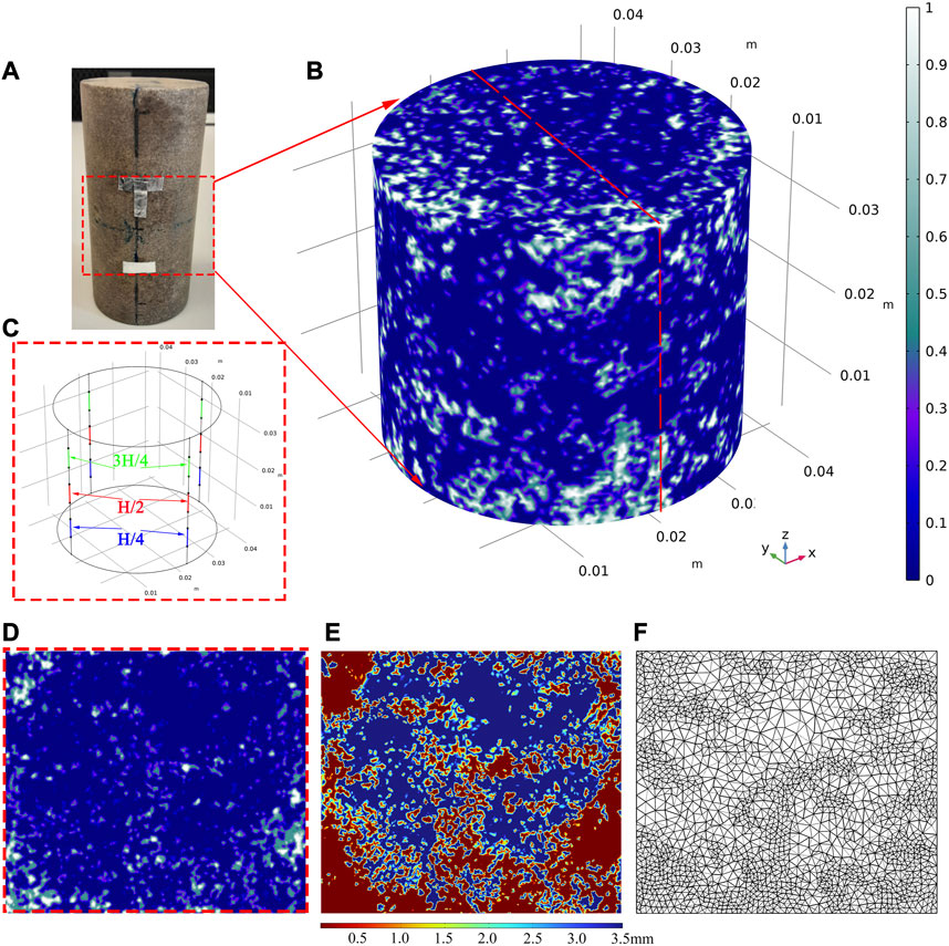
FIGURE 1. (A) Picture of the sample. The red dashed square indicates the volume that is investigated under the CT scan. The overall saturation is 88% obtained by the drainage method. More details can be found in Sun et al. (2022); (B) fluid distribution: blue zones represent regions of full water saturation. The white zones correspond to full air saturation; (C) Positions for strain gauges at 1/4 (blue), 1/2 (red), and 3/4 (green) of the sample’s length; (D) the YZ section of the fluid distribution; (E) mesh scale versus the space coordinate; (F) the adaptive mesh calculated according to (E).

2.1 Fluid distribution reconstruction

The estimation of fluid distribution is the first step of the method. For an homogenous dry sample, the fluid distribution dominates the heterogeneity of the partial saturated sample. Following Cadoret et al. (1995), recent studies like Chapman et al. (2021), Sun et al. (2022), and Wang S. et al. (2022a), the 3D fluid distribution can be estimated using the CT gray image of dry, partially and fully saturated sample. The distribution of the fluid is obtained following two steps.

(i) The gray image of partially and fully saturated samples should be normalized, referring to the gray value of two reference materials, for example, aluminum and sleeve. The rescaled image for the fully water-saturated sample can be obtained following Eq. 1, which is adapted from Lin et al. (2017) and Wang S. et al. (2022a):

${\mathrm{I}}_{cor}=\left(I-I_{ref1\_water}\right)\ast \frac{I_{ref2\_dry}-I_{ref1\_dry}}{I_{ref2\_water}-I_{ref1\_water}}+I_{ref1\_dry}(1)$

where $I_{cor}$ is the normalized gray value, $I$ is the gray value of the raw image, $I_{ref1\_water}$ and $I_{ref2\_water}$ are the average gray value of the two reference materials measured during the scan of the water-saturated sample. $I_{ref1\_dry}$ and $I_{ref2\_dry}$ are the average gray value of the two reference materials measured during the scan of the dry sample.

(ii) The images for the water-saturated sample $I_{Water}$ and partially saturated sample $I_{water+air}$ are rescaled referring to the dry sample $I_{Air}$ using Eq. 1. Then, the air saturation $S_{Air}$ is calculated as:

$S_{Air}=\frac{I_{water}-I_{water+air}}{I_{water}-I_{air}}(2)$

We use the CT data from Sun et al. (2022) obtained on an Indiana limestone partially saturated by the drainage method to calculate the fluid saturation distribution according to Eq. 1 and Eq. 2. The air saturation $S_{Air}$ is shown in Figure 1B. In this sample, the global water saturation obtained by drainage is 88%. In Figure 1B, white zones correspond to full air saturation while blue zones to pure water saturation. Air patches are distributed over the entire sample with sizes in the range of 0.5 mm–10 mm.

2.2 Numerical model meshing

The second step of the method is to mesh the fluid heterogeneities (Figure 1B). Lissa et al. (2021) converted the CT images into a surface format in AVIZO to create triangular elements on every surface between solids and pores and on the boundaries of the investigated volume. Then, they imported the mesh ‘*.stl’ in COMSOL Multiphysics. However, this procedure cannot be used for partial saturation, as shown in Figure 1B. Indeed, Figure 1B shows that the volume contains many air patches with complex geometries; in particular, the meshing process in AVIZO leads to too many intersections or overlap elements, which are difficult to remove.

We use a method presented by Cepeda et al. (2013) to overcome the limitation. This method was developed first for medical CT scan images and allows incorporating complex geometries with non-uniform material properties in COMSOL Multiphysics. It is a practical alternative, as no intersections or overlapping elements occur, and thus, it avoids the need for critical geometry simplifications that may compromise the accuracy of the simulation. In our case (Figure 1B), the non-uniform property is the fluid saturation $S_{Air}$. The mesh must be refined at the water-air interfaces. We thus define an adaptive mesh using the following steps: first, a uniform 3D cylinder is constructed according to the size of the CT image and then divided with a coarse mesh; afterward, we refine the mesh at the water-air interfaces using a function $Airarea$:

$Airarea=\frac{\left(S_{Air}^{\left(x-d,y,z\right)}+S_{Air}^{\left(x+d,y,z\right)}+S_{Air}^{\left(x,y-d,z\right)}+S_{Air}^{\left(x,y+d,z\right)}+S_{Air}^{\left(x,y,z-d\right)}+S_{Air}^{\left(x,y,z+d\right)}\right)}{6}(3)$

where, $y,$ and $\mathrm{z}$ are the space coordinates, $d$ is the fine mesh size, that is fixed. $S_{Air}^{\left(x,y,z\right)}$ denotes the air saturation at a given spatial coordinate $\left(x,y,z\right)$. For example, $S_{Air}^{\left(x-d,y,z\right)}$ signifies the air saturation at the location $\left(x-d,y,z\right)$, while $S_{Air}^{\left(x+d,y,z\right)}$ denotes the air saturation at the location $\left(x+d,y,z\right)$, and so forth. The function $Airarea$ is 1 for the air-saturated zones and 0 for the water-saturated zones and varies in the partially saturated zones. Finally, considering the 5% uncertainty in the fluid distribution, the mesh size is defined as:

$\mathrm{M}\mathrm{e}\mathrm{s}\mathrm{h}\mathrm{s}\mathrm{i}\mathrm{z}\mathrm{e}=\left\{\begin{array}{l}d,0.05\le Airarea\le 0.95\\ C,Airarea>0.95\mathrm{a}\mathrm{n}\mathrm{d}Airarea<0.05\end{array}\right.(4)$

where d and $C$ are the fine and coarse mesh sizes, respectively. Figure 1E shows the mesh size in the YZ section (Figure 1D) for the 3D fluid distribution given in Figure 1B according to Eq. 4, with C=3.5 mm and d=0.35 mm. Finally, a tetrahedral mesh is created and shown in Figure 1F. As expected, the mesh is coarse in the pure water saturation zone and refined in the partially saturated zone.

2.3 Governing equations

We use Biot’s equations (Biot, 1956a; 1956b; 1962; Rubino et al., 2009; 2016) in the frequency-space domain:

$-{\omega }^2\left({\rho }_b-\frac{{\rho }_f^2}{{\rho }_c\left(\omega \right)}\right){\mathit{u}}^{\mathit{s}}-\nabla \bullet \mathbf{\sigma }=\frac{{\rho }_f}{{\rho }_c\left(\omega \right)}\nabla P_f(5)$

$\nabla \bullet \left[-\frac{1}{{\rho }_{\mathrm{c}}\left(\omega \right)}\left(\nabla P_f-{\omega }^2{\rho }_f{\mathit{u}}^{\mathit{s}}\right)\right]-\frac{{\omega }^2{\mathit{P}}_{\mathit{f}}}{\mathrm{M}}=\alpha {\omega }^2\nabla \bullet {\mathit{u}}^{\mathit{s}}(6)$

where $\nabla$ is the Hamiltonian operator, $\omega$ is the angle frequency, $\alpha =1-\frac{K_d}{K_g}$ is Biot-Willis coefficient, $K_d$ is the drained bulk modulus, $K_g$ is the bulk modulus of the grain. The density of the saturated sample is:

${\rho }_b=\left(1-\varphi \right){\rho }_{\mathrm{s}}+\varphi {\rho }_f(7)$

where the ${\rho }_f$ and ${\rho }_{\mathrm{s}}$ are the densities of fluid and grain, respectively. $\varphi$ is the porosity. The complex density is:

${\rho }_c\left(\omega \right)=\frac{\tau {\rho }_f}{\varphi }+\frac{\eta }{\widehat{i}\omega \kappa }(8)$

where $\tau$ is the tortuosity of the pore and can be estimated roughly by $\tau =\frac{1}{2}\left(1+\frac{1}{\varphi }\right)$ according to Berryman (1982) and Rubino et al. (2009). $\eta$ is the fluid viscosity, $\kappa$ is the permeability, and $\widehat{i}$ is the imaginary unit.

The displacement vector of the rock matrix is ${\mathit{u}}^{\mathit{s}}=\left(u_i^s\right)$, and the corresponding strain tensor is defined as ${\epsilon }_{ij}=\frac{1}{2}\left(u_{i,j}^s+u_{j,i}^s\right)$, where $i,j=\mathrm{1,2,3}$ are Euclidean space dimensions.

The stress tensor $\mathrm{\sigma }$ is related to the displacement of the matrix and fluid pressure $P_f$, and:

${\sigma }_{ij}=2\mathrm{\mu }{\epsilon }_{ij}+{\delta }_{ij}\left({\lambda }_m\nabla \bullet {\mathit{u}}^{\mathit{s}}-\alpha P_f\right)(9)$

where the ${\lambda }_m=K_d-\frac{2}{3}\mathrm{\mu }$, and the $\mathrm{\mu }$ is the shear modulus, ${\delta }_{ij}=\left\{\begin{array}{c}1i=j\\ 0i\ne j\end{array}\right.$ is Kronecker (delta) tensor. The so-called pore-space modulus (Gurevich et al., 2009) is defined as:

$\mathrm{M}={\left(\frac{\varphi }{K_f}+\frac{\alpha -\varphi }{K_g}\right)}^{-1}(10)$

For a biphasic saturated sample (air/water), the effective fluid bulk modulus $K_f$, density ${\rho }_f$ and viscosity $\eta$ are defined respectively as:

$K_f={\left(\frac{S_{Air}}{K_{Air}}+\frac{1-S_{Air}}{K_w}\right)}^{-1}(11)$

${\rho }_f={\rho }_{Air}{S}_{Air}+{\rho }_w\left({1-S}_{Air}\right)(12)$

$\eta ={\eta }_{Air}{\left(\frac{{\eta }_w}{{\eta }_{Air}}\right)}^{1-S_{Air}}(13)$

where $K_{Air}$ and $K_w$ are the bulk modulus of water and air, respectively, $S_{Air}$ is the air saturation. ${\rho }_{Air}$ and ${\rho }_w$ are the densities of air and water, respectively. Eq. 13 for the mixed-fluid viscosity $\eta$ follows the work of Teja and Rice (1981), where ${\eta }_{Air}$ and ${\eta }_w$ are the viscosities of air and water, respectively.

2.4 Oscillatory relaxation test

The third step is the oscillatory relaxation test (e.g., Rubino et al., 2009; 2016; Chapman and Quintal, 2018; Santos et al., 2021).

For computing the P-wave modulus, the boundary conditions are defined as follows: i) an axial oscillation stress ${\sigma }_{33}$ is loaded at the top boundary of the sample, with an amplitude of 0.1 MPa; ii) the vertical displacement at the bottom boundary of the sample is set to zero; iii) for the side boundaries, the normal displacement is set to zero, i.e., $u_1={\mathrm{u}}_2=0$; iv) all the boundaries are impermeable for the fluid (no flow across the boundaries). The initial conditions for displacements are set to zero. The P-wave modulus ${\mathrm{M}}_P$ and P-wave attenuation $Q_P^{-1}$ are obtained using the following:

${\mathrm{M}}_P={\sigma }_{33}/{\epsilon }_{33}(14)$

$Q_P^{-1}=\mathrm{I}\mathrm{m}\mathrm{a}\mathrm{g}\left({\mathrm{M}}_P\right)/\mathrm{R}\mathrm{e}\mathrm{a}\mathrm{l}\left({\mathrm{M}}_P\right)(15)$

where ${\epsilon }_{33}$ and ${\sigma }_{33}$ are the axial strain and stress, respectively.

To compute the shear modulus (directly related to the S-velocity), the boundary conditions are defined as follows: i) an oscillation stress ${\sigma }_{32}$ is loaded at the top boundary of the sample, with an amplitude of 0.1 MPa; ii) the horizontal displacement at the bottom boundary of the sample is set to zero; iii) for the side boundaries, the axial displacement is set to zero, i.e., $u_3=0$; iv) all the boundaries are impermeable for the fluid (no flow across the boundaries). The initial conditions for displacements are set to zero. The shear modulus $\mu$ and attenuation $Q_S^{-1}$ are obtained using:

$\mu ={\sigma }_{32}/\left(2{\epsilon }_{32}\right)(16)$

$Q_S^{-1}=\mathrm{I}\mathrm{m}\mathrm{a}\mathrm{g}\left({\mathrm{M}}_S\right)/\mathrm{R}\mathrm{e}\mathrm{a}\mathrm{l}\left({\mathrm{M}}_S\right)(17)$

where ${\epsilon }_{32}$ and ${\sigma }_{32}$ are the shear strain and stress along the y direction, respectively. For both oscillatory relaxation tests, the physical properties of the rock sample and fluids used are deduced from Borgomano et al. (2019) and Sun et al. (2022) and shown in Table 1 and Table 2.

TABLE 1

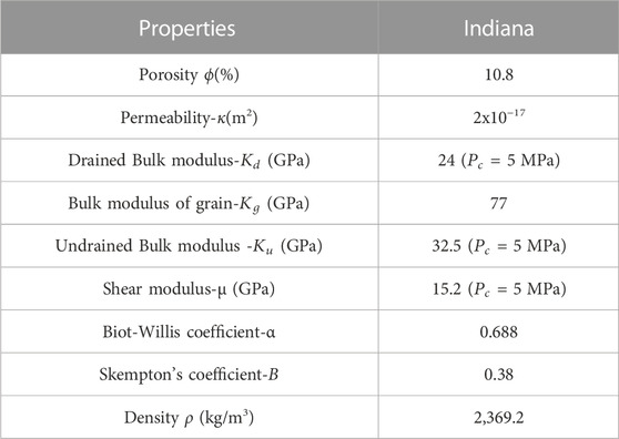
TABLE 1. Rock properties and the elastic parameters for the numerical prediction. $P_c$ is the confining pressure.

TABLE 2

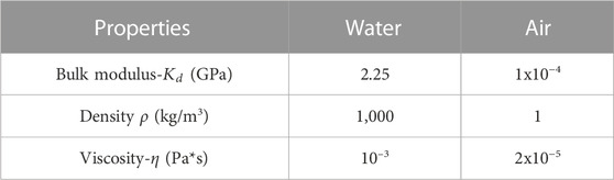
TABLE 2. Fluid properties for the numerical prediction.

Finally, the complex bulk modulus ($K$) can be deduced from the complex P-wave modulus $M_P$ and shear modulus $\mu$ by:

$K=M_P-\frac{4}{3}\mu (18)$

$Q_K^{-1}=\mathrm{I}\mathrm{m}\mathrm{a}\mathrm{g}\left(K\right)/\mathrm{R}\mathrm{e}\mathrm{a}\mathrm{l}\left(\mathrm{K}\right)(19)$

2.5 Numerical solution

The method’s fourth step is to solve Biot’s equations numerically (Eq. 5 and Eq. 6). We adopt a hybrid method (Halimi Bin Ibrahim and Skote, 2013), i.e., Newton iteration method (NIM) and LU matrix factorization method (LUM). Eq. 5 and Eq. 6 are rewritten in the following form:

$\mathit{L}\left(\mathit{X}\right)=\left(\begin{array}{c}\begin{array}{c}{L}_1\left(u_1,{\mathrm{u}}_2,{\mathrm{u}}_3,{\mathrm{P}}_{\mathrm{f}}\right)\\ L_2\left({\mathrm{u}}_1,u_2,{\mathrm{u}}_3,{\mathrm{P}}_{\mathrm{f}}\right)\end{array}\\ \begin{array}{c}{L}_3\left({\mathrm{u}}_1,{\mathrm{u}}_2,u_3,{\mathrm{P}}_{\mathrm{f}}\right)\\ L_4\left({\mathrm{u}}_1,{\mathrm{u}}_2,{\mathrm{u}}_3,P_f\right)\end{array}\end{array}\right)=0(20)$

where the variable $\mathbf{X}=\left(\begin{array}{c}\begin{array}{c}{u}_1\\ u_2\end{array}\\ \begin{array}{c}{u}_3\\ P_f\end{array}\end{array}\right)$, is composed of the solid displacement vector ${\mathit{u}}^{\mathit{s}}=$ [$\left.u_1,u_2,u_3\right]$ and fluid pressure $P_f$. Here we drop the superscript s for the solid displacement vector to leave a space for a new superscript $i$ counting the iteration number. We use a hybrid method to solve Equation 20: the displacement vector [$\left.u_1,u_2,u_3\right]$ is solved using the NIM method, and the fluid pressure $P_f$ is solved by the LUM method. The detailed steps for the hybrid method are as follows:

Step A: Set the initial condition, ${\mathbf{X}}^{\mathit{i}=\mathbf{0}}=\left(\begin{array}{c}\begin{array}{c}{u}_1^{i=0}\\ u_2^{i=0}\end{array}\\ \begin{array}{c}{u}_3^{i=0}\\ P_f^{i=0}\end{array}\end{array}\right)=0$,

Do loop on iteration number $\mathit{i}$:

Step B: Update the calculated variable $u_1^i$ ($u_1^0$ =0 for i=0). $u_1^{i+1}$ is achieved using the NIM method: The Jacobian of the linear equation $L_1$ with respect to the independent variable $u_1$ is $J_1=\frac{\partial L_1}{\partial u_1}$; then $u_1^{i+1}=u_1^i+∆u_1$, where the updated term is $∆u_1=-\frac{L_1}{J_1}$ (Ben-Israel, 1966).

Step C: Update the calculated variable $u_2^i$. $u_2^{i+1}$ is estimated using the NIM method: Take the updated $u_1^{i+1}$ into $L_2$, then calculate Jacobian $J_2=\frac{\partial L_2}{\partial u_2}$; and finally $u_2^{i+1}=u_2^i+∆u_2$ where updated term $∆u_2=-\frac{L_2}{J_2}$.

Step D: Update the calculated variable $u_3^i$. $u_3^{i+1}$ is also estimated by the NIM method: Take the updated $u_1^{i+1}$ and $u_2^{i+1}$ into $L_3$, the corresponding Jacobian is $J_3=\frac{\partial L_3}{\partial u_3}$; then $u_3^{i+1}=u_3^i+∆u_3$, where the updated term $∆u_3=-\frac{L_3}{J_3}$.

Step E: Update the calculated variable $P_f^i$. Take $u_1^{i+1}$, $u_2^{i+1}$ and $u_3^{i+1}$ into $L_4$, then $P_f^{i+1}$ is obtained using the LU matrix decomposition method (e.g., Bartels and Golub, 1969; Abbasbandy et al., 2006).

Step F: ${\mathbf{X}}^{\mathit{i}+\mathbf{1}}=\left(\begin{array}{c}\begin{array}{c}{u}_1^{i+1}\\ u_2^{i+1}\end{array}\\ \begin{array}{c}{u}_3^{i+1}\\ P_f^{i+1}\end{array}\end{array}\right)$, if $\left|{\mathbf{X}}^{\mathit{i}+\mathbf{1}}-{\mathbf{X}}^{\mathit{i}}\right|<ϵ$, end the loop; Otherwise, go back to step B and $i=i+1$. $ϵ$ is a relative error, defined as 10^–3, which is a measure of the error relative to the size of each solution component.

Figure 2 shows the evolution of the relative error for displacements and fluid pressure as a function of the iteration number during the solving process. After ten iterations, Eq. 20 is solved with a relative error below 10^–3. In the case of the hybrid method, only one independent variable is considered in every step, thus reducing the memory cost and calculation time. For comparison, we solved Eq. 20 using the hybrid method and the classical LU decomposition method and show the results in Figure 3: With the hybrid method (see the black line in Figure 3A), the memory cost is divided by a factor of 3 in comparison with the conventional LU method (see the red line in Figure 3A), and the computation time is reduced by a factor of 5 (Figure 3B).

FIGURE 2

FIGURE 2. Relative error versus iteration number during the solving process. The blue line is the fluid pressure. The green, red, and black lines correspond to displacement components along x, y, and z, respectively.

FIGURE 3

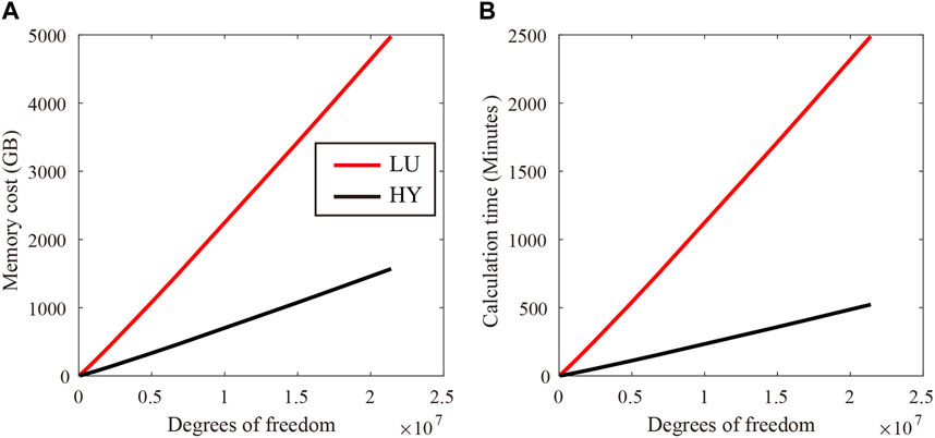
FIGURE 3. (A) Memory cost and (B) Calculation time cost. The degrees of freedom are determined by the product of the number of nodes in the mesh and the number of dependent variables (4 in our case). The black and red lines represent the hybrid method and the classical LU decomposition method, respectively.

3 Results and discussion

3.1 Axial strain ${\mathit{\epsilon }}_{\mathbf{33}}$, fluid pressure ${\mathit{P}}_{\mathit{f}}$ and local bulk modulus evolution

Using the physical properties (Table 1; Table 2) and the patchy air-water distribution (Figure 1B), we conducted an oscillatory-compressibility test (Section 2.4) to calculate the strain and fluid pressure as a function of the frequency oscillation. The distribution of the i) pore fluid pressure normalized to axial stress ${\sigma }_{33}$ and ii) axial strain are shown in Figure 4 and Figure 5, respectively, for different frequencies. It can be observed that pore pressure gradients take their highest values at the air-water interfaces with higher values for frequencies above 10 Hz. However, at the low frequency of 1Hz, air and water pressures are equilibrated to a very low value (Figure 4A). We can refer to this state as a ‘relaxed state’ under undrained conditions. Indeed, during an axial oscillation of 1Hz, the pressure of the water increases due to the Skempton effect (Kümpel, 1991), but the frequency is sufficiently low to give time for water to diffuse in the air-saturated zone, as air is much more compressible than water. At the highest frequency of 1 kHz (Figure 4D), water is pressurized and has no time to flow in the air-saturated zone, i.e., the distribution of the overpressure (red color in Figure 4D) is close to the distribution of the water saturation zones. We refer to this state as an “unrelaxed state” under undrained conditions. To estimate the increase of water pressure at 1 kHz, we recall that under the P-wave boundary condition (${\epsilon }_{11}={\epsilon }_{22}=0$), the ratio $\frac{P_f}{{\sigma }_{33}}$ in a representative elementary volume (REV) fully saturated with water is deduced as

$\frac{P_f}{{\sigma }_{33}}=B\frac{K_u}{K_u+4\mathrm{\mu }/3}(21)$

where $\mathrm{B}=\frac{1-\frac{K_d}{K_u}}{\alpha }$ is the Skempton’s coefficient (Kümpel, 1991), $\mu$ is the shear modulus. $K_u$ is the undrained bulk modulus obtained by Biot-Gassmann’s equation (Gassmann, 1951):

$K_u=K_d+{\alpha }^2{\left(\frac{\varphi }{K_f}+\frac{\alpha -\varphi }{K_g}\right)}^{-1}(22)$

FIGURE 4

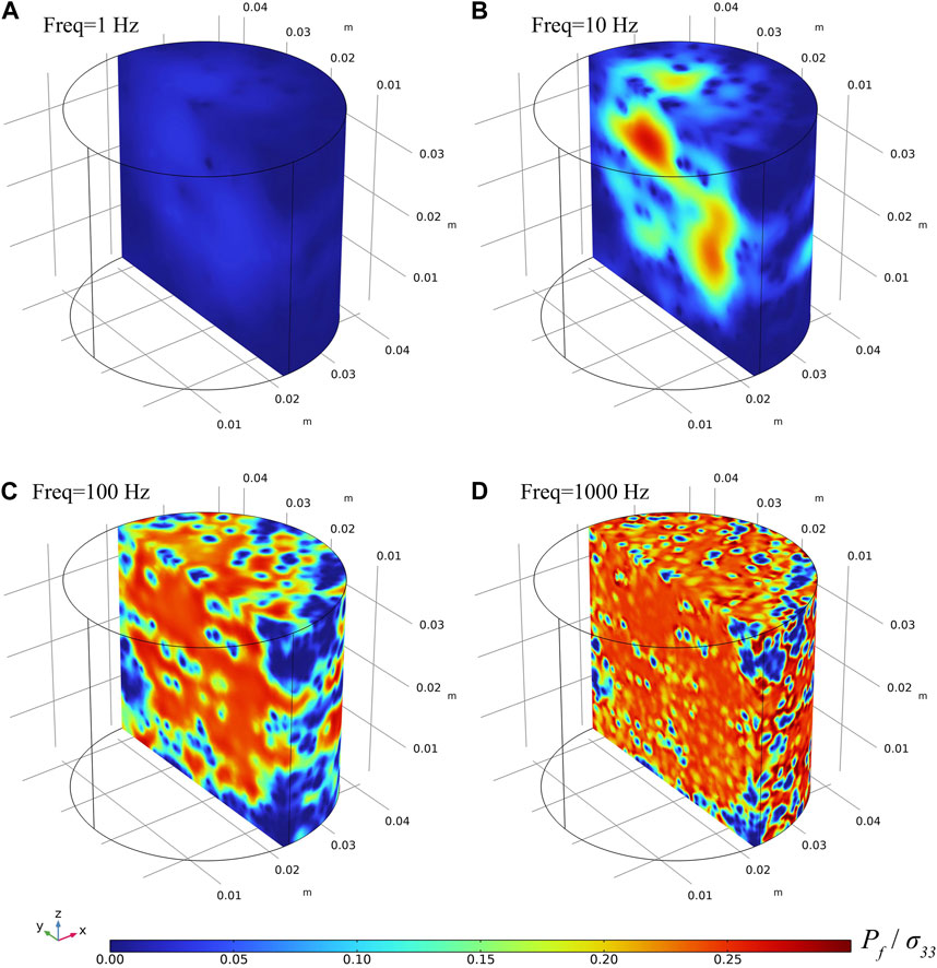
FIGURE 4. The normalized fluid pressure at frequencies of (A) 1Hz, (B) 10 Hz, (C) 100 Hz, and (D) 1,000 Hz. Total water saturation is 88% (Figure 1). The predictions are conducted using the fluid distribution shown in Figure 1 and the numerical model.

FIGURE 5

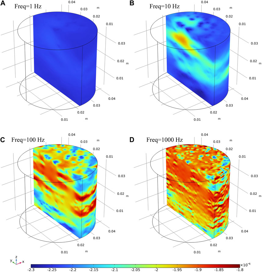
FIGURE 5. Distribution of axial strain at frequencies of (A) 1Hz, (B) 10 Hz, (C) 100 Hz and (D) 1,000 Hz. Simulations are done using the numerical test combing with the fluid distribution shown in Figure 1B.

Using the parameters given in Table 1, the Skempton’s coefficient B =0.38 and $\frac{P_f}{{\sigma }_{33}}=0.38\ast \frac{32.5}{32.5+4\ast 15.2/3}=0.23$, which is consistent with values shown in the water-saturated zones (red color in Figure 4D). For the air-saturated zones, as the compressibility of air is large, $K_u\approx K_d$ (Eq. 22 using air bulk modulus for $K_f$) and no pressurization is expected in agreement with the blue color in Figure 4D. Figure 4B and Figure 4C give the results of the water pressurization at the intermediate frequencies of 10 Hz and 100 Hz and illustrate the evolution of the pore pressure gradient in the sample as the frequency increases.

The distribution of axial strain at different frequencies is given in Figure 5. At the low frequency of 1 Hz (Figure 5A), there is no pressurization of the pore fluid (Figure 5A), and the axial deformation is homogeneous and can be approximately estimated ($K_u\approx K_d$) as:

$\left|{\epsilon }_{33}\right|=\frac{\left|{\sigma }_{33}\right|}{K_d+4\mu /3}\approx 2.3\times {10}^{-6}(23)$

which is consistent with the value predicted by the numerical simulation in Figure 5A. On the other hand, in the case of an unrelaxed state at a REV scale, the axial strain is approximately given by:

$\left|{\epsilon }_{33}\right|=\frac{\left|{\sigma }_{33}\right|}{K_u+4\mu /3}\approx 1.8\times {10}^{-6}(24)$

As a result, the axial strain varies from 2.3×10⁻⁶ to 1.8×10⁻⁶ with an increase in frequency. This signifies that the behavior of porous rock shifts from a relaxed to an unrelaxed regime at the Representative Elementary Volume (REV) scale. With the rising frequency, the spatial distribution of the axial strain undergoes changes, which align with the evolution of the pore pressure (see Figure 4; Figure 5). Specifically, areas saturated with water exhibit less deformation compared to those saturated by air. Additionally, as the frequency increases, the count of less deformable patches escalates.

Finally, we performed an oscillatory-shear test to assess the influence of frequency on pore pressure, shear strain, and shear attenuation. As anticipated, the numerical simulations indicate that oscillatory-shear stress does not induce fluid pressurization. Furthermore, shear strain is found to be independent of frequency, and there is no observable shear attenuation. This corroborates the foundational assumption in poroelasticity theory: the fluid has no effect on the shear modulus.

3.2 Global P-wave, bulk, and shear moduli

We determined the global P-wave modulus and its corresponding attenuation (represented by black curves in Figure 6A; Figure 6B), shear modulus and its corresponding attenuation (black curves in Figures 6C,D), and bulk modulus with its associated attenuation (black curves in Figure 6E; Figure 6F) by the entire specimen. These are collectively referred to as the global modulus. The four frequencies (1, 10, 100, and 1,000 Hz) highlighted in Figure 4 and Figure 5 are illustrated as red lines in Figure 6A and Figure 6B.

FIGURE 6

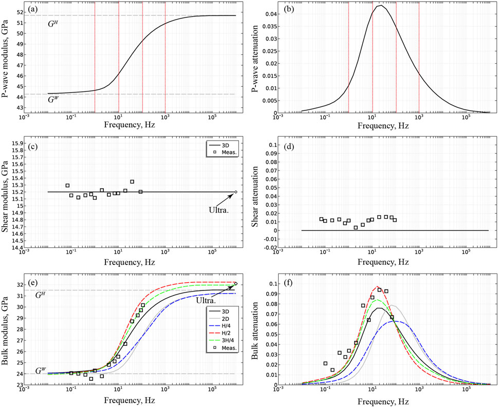
FIGURE 6. Elastic moduli of the entire sample and corresponding attenuation versus frequencies. (A) P-wave modulus; (B) P-wave attenuation; (C) shear modulus; (D) shear attenuation; (E) bulk modulus; (F) bulk attenuation. Experimental data from Sun et al. (2022) are plotted (square dots and diamond dots). The uncertainty of the measured bulk modulus is 6.4% in the seismic band and 2% at the ultrasonic frequency. In (E) and (F), in addition to the bulk modulus of the entire sample, we simulate the local bulk modulus measured by strain gauges located at the middle of the sample (red dashed line), at a quarter length from the bottom (blue dashed line) and at a quarter length from the top (green dashed lines). The Gassmann-Hill and Gassmann-wood limits are shown in (E) as dashed lines. Finally, we add a 2D numerical simulation (grey lines in (E) and (F)) to highlight the mismatch between a 2D (grey curve) and a 3D (black curve) numerical simulation.

Our initial observation revealed that the shear modulus (see Figure 6C) is independent of frequency, and there is no associated attenuation (indicating no water effect) (refer to Figure 6D). On the other hand, the bulk modulus (represented by the black curves in Figure 6E) ranges from 24.2 GPa to 31.3 GPa. This span corresponds to the bulk modulus in both the relaxed and unrelaxed states under the undrained boundary condition (see Figure 6).

At lower frequencies, the fluid pressure has ample time to equilibrate, yielding a homogeneously mixed fluid. Consequently, the bulk modulus of this mixed fluid can be treated as a single-phase effective fluid bulk modulus by applying Wood’s law (1946):

${K_f^{LF}=\left(\frac{1-S}{K_{air}}+\frac{S}{K_{wat}}\right)}^{-1}(25)$

Here, S represents the water saturation. S=0.88, $K_{air}$ =10^–4 GPa, and $K_{wat}$ =2.25 GPa. This results in $K_f^{LF}=$ 8x10⁻⁴ GPa, which is approximately equal to $K_{air}$. By extending Gassmann’s theory (as per Eq. 22) with $K_f^{LF}$, we infer a bulk modulus (24.2 GPa) that closely mirrors the drained bulk modulus (24 GPa). This represents the minimum value for the bulk modulus, often referred to as the low-frequency limit or the Gassmann-Wood limit.

At higher frequencies, there is insufficient time for fluid flow and pressure equalization. Under these conditions, individual fluid phases are effectively isolated, allowing for the use of Eq. 22 to define an undrained bulk modulus for each region saturated by its respective fluid. Following this, Hill’s law (1963) can be used to define an effective bulk modulus for the entire sample:

$K^{HF}={\left(\frac{S}{K_u+4/3\mu }+\frac{1-S}{K_d+4/3\mu }\right)}^{-1}-4/3\mu (26)$

Here, $K_d$ represents the drained bulk modulus and $K_u$ is the undrained bulk modulus fully saturated with water (Mavko and Mukerji, 1998). This upper limit, referred to as the Gassmann-Hill limit, results in $K^{HF}=$ 31.3 GPa in our case, which is less than $K_u=32.5$ GPa. Both the drained bulk modulus and the Gassmann-Hill limit are depicted as dashed grey lines in Figure 6E.

In a short summary, the bulk modulus of the entire sample escalates from the Gassmann-Wood limit to the Gassmann-Hill limit with increasing frequency. The dispersion is associated with an attenuation (represented by the black curve in Figure 6F) peaking at 0.075 at 20 Hz. Lastly, we plot the P-wave modulus and its corresponding attenuation as functions of frequency in Figures 6A,B. As the P-wave modulus is a linear amalgamation of the shear and bulk moduli, its behavior closely mirrors that of the bulk modulus. Specifically, the P-wave modulus increases from 44 GPa to 52 GPa, accompanied by a peak attenuation of 0.045 at 20 Hz.

3.3 Numerical prediction vs experimental measurements

In numerous laboratory experiments (e.g., Batzle et al., 2006; Adelinet et al., 2010; Mikhaltsevitch et al., 2015; Sun et al., 2018), researchers measure the strain’s evolution with frequency under oscillatory stress using local strain gauges. This approach yields a locally measured bulk modulus. To emulate such experiments, we average strain over a span of 6 mm—the typical length of a strain gauge—and simulate four strain gauges that are averaged. These gauges are situated at the sample’s half-length (represented by red lines in Figure 1C), a quarter-length from the bottom (blue lines in Figure 1C), and a quarter-length from the top (green lines in Figure 1C). The results are presented in Figure 6E: In general, the local bulk modulus and attenuation measured at the midpoint (50%, red curve) and three-quarters (75%, green curve) of the sample length closely align with the bulk properties of the entire sample (black curve). However, the frequency-dependent evolution of the local bulk modulus at one-quarter (25%, blue curve) of the sample deviates significantly from the evolution of the global bulk modulus (black curve). Furthermore, the high-frequency limit of local measurements differs from the Gassmann-Hill limit, as the strain gauges only capture the effects of local saturation. Consequently, high-frequency results may approach the undrained bulk modulus fully saturated with water, which surpasses the Gassmann-Hill limit. Interestingly, the disparity between local and global measurements in our study is not as marked as in Chapman and Quintal (2018). This reduced difference can likely be attributed to i) our approach of consolidating local results from four strain gauges, which serves to lessen the discrepancy between local and global responses, and ii) a comparatively uniform air/water distribution in our experiment, as opposed to the more varied distribution seen in Chapman and Quintal’s work (2018).

The progression of the moduli with frequency for the Indiana sample, saturated to 88% (Figures 1A,B), was studied by Sun et al., 2022. We chose the Indiana sample for this investigation due to its lack of micro-cracks, thus eliminating the squirt-flow mechanism (Borgomano et al., 2019). In these tests, strain measurements were taken by averaging readings from four strain gauges situated in the half-length of the specimen. We have represented the experimental data in Figure 6 with black square dots. Figures 6C,D juxtapose the projected and observed values of the shear modulus and attenuation. The frequency-independent shear modulus (depicted by the black curve in Figure 6C) aligns with the measurements (square dots in Figure 6C) spanning the seismic bands (0.1–100 Hz) and ultrasonic frequency (1 MHz). Additionally, the predicted shear attenuation (black curve in Figure 6D) aligns with the measurement (square dots in Figure 6D), given that the measurement error range for attenuation is within 0.02.

Figures 6E,F juxtapose the anticipated and actual measurements of the bulk modulus and attenuation. Generally, there’s an excellent agreement between the measurements and the numerical predictions, as illustrated by the black square dots and red curves. The numerical simulation, based on the CT-scan images, accurately replicates i) the dispersion of the modulus and ii) both the low and high-frequency limit. There’s also a strong correspondence between the measured attenuation and the numerical simulation. This comparison between the numerical simulation and experimental data confirms the efficacy of the method detailed in this paper in predicting mesoscopic dispersion and attenuation.

3.4 2D model vs 3D model

We now turn to comparing the results derived from 2D and 3D numerical simulations. Utilizing the YZ section of the CT image (Figure 1D), the bulk modulus and attenuation for the 2D model were computed. The global response of the 2D model is determined by averaging the strain across the entire section. As shown by the solid gray line in Figure 6F, the prediction using the 2D model exhibits a higher critical frequency (100 Hz) and peak attenuation (0.08) compared to the 3D model (black curve in Figure 6F). Furthermore, the bulk modulus derived from the 2D model (solid gray line in Figure 6E) deviates from the one obtained from the 3D model (black curve in Figure 6E). The discrepancy between the 2D and 3D results is attributed to the fluid flow in the ZX and ZY direction, which is not accounted for in the 2D numerical simulation. This finding elucidates the mismatch observed by Sun et al. (2022) between experimental data and numerical simulation, which can be attributed to their use of a 2D model.

4 Conclusion

In this paper, we introduce a novel method aimed at predicting velocity dispersion and attenuation attributable to mesoscopic flow, leveraging actual fluid distribution data derived from CT images. The numerical model is initially established by meshing CT images through a technique adept at handling intricate geometries and non-uniform material properties, thus effectively bypassing element intersections, a common issue associated with AVIZO. To find the solution for the numerical model governed by Biot’s equations, we use a hybrid method that significantly curtails memory cost compared to the LU matrix factorization method.

The solution from the numerical model forecasts the evolution of pore pressure distribution with frequency, thereby anticipating the advancement of the elastic moduli and their attenuation. We also model the development of the moduli for the entire sample (global moduli) as well as those measured by a strain gauge (local moduli). The discrepancies observed between local and global responses can be attributed to the heterogeneity in fluid distribution. Importantly, the 3D model’s predictions are validated by experimental data collected from Indiana limestone.

The presented method successfully addresses issues pertaining to memory consumption and calculation time, thereby setting the stage for quantifying the relationship between fluid distribution and seismic attenuation. This innovative approach holds the potential to serve as a robust tool for upscaling at the reservoir scale.

Data availability statement

The raw data supporting the conclusion of this article will be made available by the authors, without undue reservation.

Author contributions

CS: Methodology, Writing–original draft, Writing–review and editing. JF: Methodology, Writing–original draft, Writing–review and editing. GT: Supervision, Writing–review and editing. SW: Supervision, Writing–review and editing.

Funding

The author(s) declare financial supportwas received for the research, authorship, and/or publication of this article. This work is supported by the National Natural Science Foundation of China (42104111, 42274142, 41930425, 41774143, 41804104) and also supported by Open Fund (WX-KFJJ-2022-08) of SINOPEC Key Laboratory of Geophysics, and State Key Laboratory of Petroleum Resources and Prospecting, China University of Petroleum, and Xuzhou Science and Technology Bureau Young Talents Project (No. KC22018). The authors declare that this study received funding from SINOPEC Key Laboratory of Geophysics. The funder was not involved in the study design, collection, analysis, interpretation of data, the writing of this article, or the decision to submit it for publication.

Acknowledgments

We acknowledge the help of Dr. Jan V. M. Borgomano at Ecole Normale Supérieure for scanning the sample.

Conflict of interest

Authors GT and SW were employed by China National Petroleum Corporation.

The remaining authors declare that the research was conducted in the absence of any commercial or financial relationships that could be construed as a potential conflict of interest.

Publisher’s note

All claims expressed in this article are solely those of the authors and do not necessarily represent those of their affiliated organizations, or those of the publisher, the editors and the reviewers. Any product that may be evaluated in this article, or claim that may be made by its manufacturer, is not guaranteed or endorsed by the publisher.

References

Abbasbandy, S., Ezzati, R., and Jafarian, A. (2006). LU decomposition method for solving fuzzy system of linear equations. Appl. Math. Comput. 172 (1), 633–643. doi:10.1016/j.amc.2005.02.018

CrossRef Full Text | Google Scholar

Adelinet, M., Dorbath, C., Ravalec, M. L., Fortin, J., and Guéguen, Y. (2011). Deriving microstructure and fluid state within the Icelandic crust from the inversion of tomography data. Geophys. Res. Lett. 38 (3). doi:10.1029/2010GL046304

CrossRef Full Text | Google Scholar

Adelinet, M., Fortin, J., Guéguen, Y., Schubnel, A., and Geoffroy, L. (2010). Frequency and fluid effects on elastic properties of basalt: experimental investigations. Geophys. Res. Lett. 37 (2). doi:10.1029/2009GL041660

CrossRef Full Text | Google Scholar

Anwer, H. M., Ali, A., and Alves, T. M. (2017). Bayesian inversion of synthetic AVO data to assess fluid and shale content in sand-shale media. J. Earth Syst. Sci. 126 (3), 42. doi:10.1007/s12040-017-0818-y

CrossRef Full Text | Google Scholar

Ba, J., Carcione, J. M., and Sun, W. (2015). Seismic attenuation due to heterogeneities of rock fabric and fluid distribution. Geophys. J. Int. 202 (3), 1843–1847. doi:10.1093/gji/ggv255

CrossRef Full Text | Google Scholar

Ba, J., Xu, W., Fu, L.-Y., Carcione, J. M., and Zhang, L. (2017). Rock anelasticity due to patchy saturation and fabric heterogeneity: A double double-porosity model of wave propagation. J. Geophys. Res. Solid Earth 122 (3), 1949–1976. doi:10.1002/2016JB013882

CrossRef Full Text | Google Scholar

Bartels, R. H., and Golub, G. H. (1969). The simplex method of linear programming using LU decomposition. Commun. ACM 12 (5), 266–268. doi:10.1145/362946.362974

CrossRef Full Text | Google Scholar

Batzle, M. L., Han, D.-H., and Hofmann, R. (2006). Fluid mobility and frequency-dependent seismic velocity — direct measurements. GEOPHYSICS 71 (1), N1–N9. doi:10.1190/1.2159053

CrossRef Full Text | Google Scholar

Ben-Israel, A. (1966). A Newton-Raphson method for the solution of systems of equations. J. Math. Analysis Appl. 15 (2), 243–252. doi:10.1016/0022-247X(66)90115-6

CrossRef Full Text | Google Scholar

Berryman (1982). “Elastic waves in fluid-saturated porous media (Vol 154),” in Macroscopic Properties of Disordered Media, Rome, June 1–3, 1981.

Google Scholar

Biot, M. A. (1962). Mechanics of deformation and acoustic propagation in porous media. J. Appl. Phys. 33 (4), 1482–1498. doi:10.1063/1.1728759

CrossRef Full Text | Google Scholar

Biot, M. A. (1956b). Theory of propagation of elastic waves in a fluid-saturated porous solid. II. Higher frequency range. J. Acoust. Soc. Am. 28 (2), 179–191. doi:10.1121/1.1908241

CrossRef Full Text | Google Scholar

Biot, M. A. (1956a). Theory of propagation of elastic waves in a fluid-saturated porous solid. I. Low-Frequency range. J. Acoust. Soc. Am. 28 (2), 168–178. doi:10.1121/1.1908239

CrossRef Full Text | Google Scholar

Borgomano, J. V. M., Pimienta, L. X., Fortin, J., and Guéguen, Y. (2019). Seismic dispersion and attenuation in fluid-saturated carbonate rocks: effect of microstructure and pressure. J. Geophys. Res. Solid Earth 124 (12), 12498–12522. doi:10.1029/2019JB018434

CrossRef Full Text | Google Scholar

Chapman, S., and Quintal, B. (2018). “Numerical assessment of local versus bulk strain measurements to quantify seismic attenuation in partially saturated rocks,” in SEG technical program expanded abstracts 2018 (Texas, United States: Society of Exploration Geophysicists), 1–0, 3547–3551. doi:10.1190/segam2018-2992202.1

PubMed Abstract | CrossRef Full Text | Google Scholar

Cadoret, T., Mavko, G., and Zinszner, B. (1998). Fluid distribution effect on sonic attenuation in partially saturated limestones. GEOPHYSICS 63 (1), 154–160. doi:10.1190/1.1444308

CrossRef Full Text | Google Scholar

Cadoret, T., Marion, D., and Zinszner, B. (1995). Influence of frequency and fluid distribution on elastic wave velocities in partially saturated limestones. J. Geophys. Res. Solid Earth 100 (B6), 9789–9803. doi:10.1029/95JB00757

CrossRef Full Text | Google Scholar

Cavallini, F., Carcione, J. M., Vidal de Ventós, D., and Engell-Sørensen, L. (2017). Low-frequency dispersion and attenuation in anisotropic partially saturated rocks. Geophys. J. Int. 209 (3), 1572–1584. doi:10.1093/gji/ggx107

CrossRef Full Text | Google Scholar

Cepeda, J. F., Birla, S., Subbiah, J., and Thippareddi, H. (2013). A practical method to model complex three-dimensional geometries with non-uniform material properties using image-based design and COMSOL multiphysics.

Google Scholar

Chapman, S., Borgomano, J. V. M., Quintal, B., Benson, S. M., and Fortin, J. (2021). Seismic wave attenuation and dispersion due to partial fluid saturation: direct measurements and numerical simulations based on x-ray ct. J. Geophys. Res. Solid Earth 126 (4). doi:10.1029/2021JB021643

CrossRef Full Text | Google Scholar

Chapman, S., Tisato, N., Quintal, B., and Holliger, K. (2016). Seismic attenuation in partially saturated berea sandstone submitted to a range of confining pressures: seismic attenuation in berea sandstone. J. Geophys. Res. Solid Earth 121 (3), 1664–1676. doi:10.1002/2015JB012575

CrossRef Full Text | Google Scholar

Dutta, N. C., and Odé, H. (1979). Attenuation and dispersion of compressional waves in fluid-filled porous rocks with partial gas saturation (White model); Part II, Results. Geophysics 44 (11), 1789–1805. doi:10.1190/1.1440939

CrossRef Full Text | Google Scholar

Gassmann, F. (1951). Über die elastizität poröser medien: vier. der natur. Ges. Zürich 96, 1–23.

Google Scholar

Gurevich, B., Brajanovski, M., Galvin, R. J., Müller, T. M., and Toms-Stewart, J. (2009). P-wave dispersion and attenuation in fractured and porous reservoirs – poroelasticity approach. Geophys. Prospect. 57 (2), 225–237. doi:10.1111/j.1365-2478.2009.00785.x

CrossRef Full Text | Google Scholar

Halimi Bin Ibrahim, I., and Skote, M. (2013). Effects of the scalar parameters in the Suzen-Huang model on plasma actuator characteristics. Int. J. Numer. Methods Heat Fluid Flow 23 (6), 1076–1103. doi:10.1108/HFF-05-2011-0108

CrossRef Full Text | Google Scholar

He, Y.-X., Wang, S., Yuan, S., Tang, G., and Wu, X. (2020). An improved approach for hydrocarbon detection using Bayesian inversion of frequency- and angle-dependent seismic signatures of highly attenuative reservoirs. IEEE Geoscience Remote Sens. Lett. 19, 1–5. doi:10.1109/LGRS.2020.3017627

CrossRef Full Text | Google Scholar

Hill, R. (1963). Elastic properties of reinforced solids: some theoretical principles. J. Mech. Phys. Solids 11 (5), 357–372. doi:10.1016/0022-5096(63)90036-X

CrossRef Full Text | Google Scholar

Klimentos, T. (1995). Attenuation of P- and S-waves as a method of distinguishing gas and condensate from oil and water. GEOPHYSICS 60 (2), 447–458. doi:10.1190/1.1443782

CrossRef Full Text | Google Scholar

Kümpel, H.-J. (1991). Poroelasticity: parameters reviewed. Geophys. J. Int. 105 (3), 783–799. doi:10.1111/j.1365-246X.1991.tb00813.x

CrossRef Full Text | Google Scholar

Lin, Q., Bijeljic, B., Raeini, A. Q., Rieke, H., and Blunt, M. J. (2021). Drainage capillary pressure distribution and fluid displacement in a heterogeneous laminated sandstone. Geophys. Res. Lett. 48 (14), e2021GL093604. doi:10.1029/2021GL093604

CrossRef Full Text | Google Scholar

Lin, Q., Bijeljic, B., Rieke, H., and Blunt, M. J. (2017). Visualization and quantification of capillary drainage in the pore space of laminated sandstone by a porous plate method using differential imaging X-ray microtomography: imaging of capillary drainage using dipp. Water Resour. Res. 53 (8), 7457–7468. doi:10.1002/2017WR021083

CrossRef Full Text | Google Scholar

Lissa, S., Ruf, M., Steeb, H., and Quintal, B. (2021). Digital rock physics applied to squirt flow. GEOPHYSICS 86 (4), MR235–MR245. doi:10.1190/geo2020-0731.1

CrossRef Full Text | Google Scholar

Mavko, G., and Mukerji, T. (1998). Bounds on low-frequency seismic velocities in partially saturated rocks. GEOPHYSICS 63 (3), 918–924. doi:10.1190/1.1444402

CrossRef Full Text | Google Scholar

Mikhaltsevitch, V., Lebedev, M., and Gurevich, B. (2016). Laboratory measurements of the effect of fluid saturation on elastic properties of carbonates at seismic frequencies: effect of fluid saturation on carbonates. Geophys. Prospect. 64 (4), 799–809. doi:10.1111/1365-2478.12404

CrossRef Full Text | Google Scholar

Mikhaltsevitch, V., Lebedev, M., and Gurevich, B. (2015). A laboratory study of attenuation and dispersion effects in glycerol-saturated Berea sandstone at seismic frequencies. Texas, United States: Society of Exploration Geophysicists, 3085–3089. doi:10.1190/segam2015-5898429.1

CrossRef Full Text | Google Scholar

Monachesi, L. B., Wollner, U., and Dvorkin, J. (2020). Effective pore fluid bulk modulus at patchy saturation: an analytic study. J. Geophys. Res. Solid Earth 125 (1), e2019JB018267. doi:10.1029/2019JB018267

CrossRef Full Text | Google Scholar

Müller, T. M., Toms-Stewart, J., and Wenzlau, F. (2008). Velocity-saturation relation for partially saturated rocks with fractal pore fluid distribution. Geophys. Res. Lett. 35 (9), L09306. doi:10.1029/2007GL033074

CrossRef Full Text | Google Scholar

Müller, T. M., Gurevich, B., and Lebedev, M. (2010). Seismic wave attenuation and dispersion resulting from wave-induced flow in porous rocks A review. Geophysics 75 (5), 75A147–75A164. doi:10.1190/1.3463417

CrossRef Full Text | Google Scholar

Müller, T. M., and Gurevich, B. (2004). One-dimensional random patchy saturation model for velocity and attenuation in porous rocks. Geophysics 69 (5), 1166–1172. doi:10.1190/1.1801934

CrossRef Full Text | Google Scholar

Müller, T. M., and Gurevich, B. (2005). Wave-induced fluid flow in random porous media: attenuation and dispersion of elastic waves. J. Acoust. Soc. Am. 117 (5), 2732–2741. doi:10.1121/1.1894792

PubMed Abstract | CrossRef Full Text | Google Scholar

Pride, S. R., Berryman, J. G., and Harris, J. M. (2004). Seismic attenuation due to wave-induced flow. J. Geophys. Res. Solid Earth 109 (B1), B01201. doi:10.1029/2003JB002639

CrossRef Full Text | Google Scholar

Qi, Q., Müller, T. M., Gurevich, B., Lopes, S., Lebedev, M., and Caspari, E. (2014). Quantifying the effect of capillarity on attenuation and dispersion in patchy-saturated rocks. GEOPHYSICS 79 (5), WB35–WB50. doi:10.1190/geo2013-0425.1

CrossRef Full Text | Google Scholar

Quintal, B., Frehner, M., Madonna, C., Tisato, N., Kuteynikova, M., and Saenger, E. H. (2011). Integrated numerical and laboratory rock physics applied to seismic characterization of reservoir rocks. Lead. Edge 30 (12), 1360–1367. doi:10.1190/1.3672480

CrossRef Full Text | Google Scholar

Rubino, J. G., Caspari, E., Müller, T. M., Milani, M., Barbosa, N. D., and Holliger, K. (2016). Numerical upscaling in 2-D heterogeneous poroelastic rocks: anisotropic attenuation and dispersion of seismic waves. J. Geophys. Res. Solid Earth 121 (9), 6698–6721. doi:10.1002/2016JB013165

CrossRef Full Text | Google Scholar

Rubino, J. G., Ravazzoli, C. L., and Santos, J. E. (2009). Equivalent viscoelastic solids for heterogeneous fluid-saturated porous rocks. GEOPHYSICS 74 (1), N1–N13. doi:10.1190/1.3008544

CrossRef Full Text | Google Scholar

Santos, J., Carcione, J., and Ba, J. (2021). Two-phase flow effects on seismic wave anelasticity in anisotropic poroelastic media. Energies 14 (20), 6528. doi:10.3390/en14206528

CrossRef Full Text | Google Scholar

Santos, J. E., Ravazzoli, C. L., Gauzellino, P. M., and Carcione, J. M. (2005). Numerical simulation of ultrasonic waves in reservoir rocks with patchy saturation and fractal petrophysical properties. Comput. Geosci. 9 (1), 1–27. doi:10.1007/s10596-005-2848-9

CrossRef Full Text | Google Scholar

Sun, C., Fortin, J., Borgomano, J. V. M., Wang, S., Tang, G., Bultreys, T., et al. (2022). Influence of fluid distribution on seismic dispersion and attenuation in partially saturated limestone. J. Geophys. Res. Solid Earth 127 (5). doi:10.1029/2021JB023867

CrossRef Full Text | Google Scholar

Sun, C., Tang, G., Zhao, J., Zhao, L., and Wang, S. (2018). An enhanced broad-frequency-band apparatus for dynamic measurement of elastic moduli and Poisson’s ratio of rock samples. Rev. Sci. Instrum. 89 (6), 064503. doi:10.1063/1.5018152

PubMed Abstract | CrossRef Full Text | Google Scholar

Sun, W. (2017). Determination of elastic moduli of composite medium containing bimaterial matrix and non-uniform inclusion concentrations. Appl. Math. Mech. 38 (1), 15–28. doi:10.1007/s10483-017-2157-6

CrossRef Full Text | Google Scholar

Teja, A. S., and Rice, P. (1981). Generalized corresponding states method for the viscosities of liquid mixtures. Industrial Eng. Chem. Fundam. 20 (1), 77–81. doi:10.1021/i100001a015

CrossRef Full Text | Google Scholar

Tester, J. W., Anderson, B. J., Batchelor, A. S., Blackwell, D. D., DiPippo, R., Drake, E. M., et al. (2007). Impact of enhanced geothermal systems on US energy supply in the twenty-first century. Philosophical Trans. R. Soc. A Math. Phys. Eng. Sci. 365 (1853), 1057–1094. doi:10.1098/rsta.2006.1964

PubMed Abstract | CrossRef Full Text | Google Scholar

Tisato, N., and Quintal, B. (2013). Measurements of seismic attenuation and transient fluid pressure in partially saturated berea sandstone: evidence of fluid flow on the mesoscopic scale. Geophys. J. Int. 195 (1), 342–351. doi:10.1093/gji/ggt259

CrossRef Full Text | Google Scholar

Toms, J., Müller, T. M., and Gurevich, B. (2007). Seismic attenuation in porous rocks with random patchy saturation. Geophys. Prospect. 55 (5), 671–678. doi:10.1111/j.1365-2478.2007.00644.x

CrossRef Full Text | Google Scholar

Toms-Stewart, J., Müller, T. M., Gurevich, B., and Paterson, L. (2009). Statistical characterization of gas-patch distributions in partially saturated rocks. GEOPHYSICS 74 (2), WA51–WA64. doi:10.1190/1.3073007

CrossRef Full Text | Google Scholar

Wang, S., Ruspini, L. C., Øren, P.-E., Van Offenwert, S., and Bultreys, T. (2022a). Anchoring multi-scale models to micron-scale imaging of multiphase flow in rocks. Water Resour. Res. 58 (1), e2021WR030870. doi:10.1029/2021WR030870

CrossRef Full Text | Google Scholar

Wang, Y., Zhao, L., Cao, C., Yao, Q., Yang, Z., Cao, H., et al. (2022b). Wave-induced fluid pressure diffusion and anelasticity in partially saturated rocks: the influences of boundary conditions. Geophysics 87 (5), MR247–MR263. doi:10.1190/geo2021-0809.1

CrossRef Full Text | Google Scholar

White, J. E. (1975). Computed seismic speeds and attenuation in rocks with partial gas saturation. Geophysics 40 (2), 224–232. doi:10.1190/1.1440520

CrossRef Full Text | Google Scholar

White, J. E., Mihailova, N., and Lyakhovitsky, F. (1975). Low-frequency seismic waves in fluid-saturated layered rocks. J. Acoust. Soc. Am. 57 (S1), S30. doi:10.1121/1.1995164

CrossRef Full Text | Google Scholar

Wood, A. B. (1946). A textbook of sound. 2. New York: Macmillan. Available at: http://archive.org/details/in.ernet.dli.2015.15768.

Google Scholar

Zhang, L., Ba, J., Carcione, J. M., and Wu, C. (2022). Seismic wave propagation in partially saturated rocks with a fractal distribution of fluid-patch size. J. Geophys. Res. Solid Earth 127 (2). doi:10.1029/2021JB023809

CrossRef Full Text | Google Scholar

Zhao, L., Tang, G., Sun, C., Zhao, J., and Wang, S. (2021a). Dual attenuation peaks revealing mesoscopic and microscopic fluid flow in partially oil-saturated Fontainebleau sandstones. Geophys. J. Int. 224 (3), 1670–1683. doi:10.1093/gji/ggaa551

CrossRef Full Text | Google Scholar

Zhao, L., Wang, Y., Yao, Q., Geng, J., Li, H., Yuan, H., et al. (2021b). Extended Gassmann equation with dynamic volumetric strain: modeling wave dispersion and attenuation of heterogeneous porous rocks. Geophysics 86 (3), MR149–MR164. doi:10.1190/geo2020-0395.1

CrossRef Full Text | Google Scholar

Zhu, W., Zhao, L., and Shan, R. (2017). Modeling effective elastic properties of digital rocks using a new dynamic stress-strain simulation method. Geophysics 82 (6), MR163–MR174. doi:10.1190/geo2016-0556.1

CrossRef Full Text | Google Scholar

Zhu, W., Zhao, L., Yang, Z., Cao, H., Wang, Y., Chen, W., et al. (2023). Stress relaxing simulation on digital rock: characterize attenuation due to wave-induced fluid flow and scattering. J. Geophys. Res. Solid Earth 128 (2), e2022JB024850. doi:10.1029/2022jb024850

CrossRef Full Text | Google Scholar