 Yao Zhang
- College of Civil Engineering and Architecture, Zhejiang University of Water Resources and Electric Power, Hangzhou, China
Fault slip rates are critical parameters for assessing regional strain accumulation and seismic hazards. Previous investigations on fault slip rates primarily concentrated on shallow depths or along the strike of the fault, neglecting the variation with depth. This study focuses on listric normal faults, commonly observed in tectonic extensional zones, and investigates the variation of slip rates with depth. The relationships between slip rates along different fault segments are derived based on the inclined shear geometric models. The study finds that slip rates on different segments of listric normal faults are generally not equal and depend on the type of bend (concave or convex), the dip angles of the fault segments and axial surfaces. Inferring regional horizontal extension solely from shallow segment displacements or growth strata thickness may lead to inaccurate conclusions. In accordance with the methodology outlined in this paper, slip rates at various depths along the Chengnan Fault for the three time intervals: 24.6–33 Ma, 33–43.5 Ma, and 43.5–65 Ma, are estimated. The results of this study offer valuable insights into the kinematics of listric normal faults, facilitating a better comprehension of the discrepancy between slip rates measured at surface and slip rates measured at depth.
1 Introduction
The fault slip rate could be calculated by dividing the accumulated displacement by the timing of the displacement. Displacement is measured from geomorphic markers, trenching, gravity modeling and interpretation of seismic reflection data, whilst the timing of the displacement is determined by radiocarbon dating, tephrachronology, fission track dating and identification of fossils. The fault slip rate is a very important kinematic parameter of active faults, as it can be applied to evaluate regional strain accumulation and estimate seismic hazards (Anderson et al., 1996; Nicol et al., 1997; Galadini and Galli, 2000; Nicol et al., 2005; Nicol et al., 2006; Mouslopoulou et al., 2009; Blakeslee and Kattenhorn, 2013).
Listric normal faults are commonly observed in tectonic extensional zones. There have been numerous studies on fault slip rates of listric normal faults by previous researchers, revealing that fault slip rates vary with lateral position and time (Mitchell et al., 2001; Benedetti et al., 2002; Friedrich et al., 2003; Bull et al., 2006; Nicol et al., 2006; McClymont et al., 2009; Schlagenhauf et al., 2010; Schlagenhauf et al., 2011). Previous investigations indicate many listric normal faults show curvature in plan view, and slip rate is larger in the center along a fault trace than it is at the ends of a fault (Nicol et al., 2010; Zhang et al., 2020). However, how fault slip rates vary at different depths has been poorly studied. The variation of slip rate with depth in listric normal faults is an essential aspect to consider when studying the mechanics of faulting and earthquake generation, as it influences the overall seismic behavior and deformation pattern within the fault zone. When using fault slip rates to estimate the average earthquake frequency, it is necessary to assume that surface measurements of slip rate represent slip rates at seismogenic depths (Youngs and Coppersmith, 1985). Understanding this variation is crucial for assessing seismic hazards and for developing accurate models of fault behavior in tectonically active regions. Therefore, the objective of this study is to investigate whether there are differences between surface fault slip rates and those at subsurface levels of listric normal faults based on geometric models, as well as to identify the factors controlling these differences.
2 Methods
The inclined shear model is employed to analyze the relationship between slip rates at different depths in listric normal faults, as this model is the predominant deformation mode for listric normal faults (Dula, 1991; Xiao and Suppe, 1992). Forward modeling and geometric analysis methods were extensively employed in this study. The following introduces the inclined shear model of listric normal faults.
Assuming the presence of a normal fault with a single concave bend, as the hanging wall moves, if the hanging wall has a significantly high strength, it will remain undeformed and a gap will develop between the hanging wall and the footwall (Figure 1A). However, in reality, the hanging wall does not possess sufficient strength, resulting in its collapse and subsequent filling of the gap. Extensive research has demonstrated that antithetic normal faulting is a prevalent mechanism for the collapse deformation of the hanging wall (Figure 1B; White et al., 1986; Groshong, 1989; Dula, 1991; White and Yielding, 1991; Kerr and White, 1992; White, 1992; Xiao and Suppe, 1992; Withjack and Peterson, 1993; Withjack et al., 1995; Hauge and Gray, 1996; Withjack and Schlische, 2006). The collapse of the hanging wall of a fault induces tilting deformation of the strata, giving rise to a kink band comprising dipping beds. This kink band is delineated by two axial surfaces aligned in the direction of hanging wall collapse. Axial surface AB is located at the inflection point of the fault. Although it remains stationary relative to the footwall and the fault, it is an active axial surface. This is because as the slip distance of the fault increases, the strata of the hanging wall pass through this surface and undergo tilting deformation. The initial position of axial surface A′B′ coincides with axial surface AB. As the fault slips, axial surface A′B′ moves along with the fault displacement. Axial surface A′B′ is an inactive axial surface because its position remains fixed relative to the hanging wall, and no new strata undergo deformation by passing through this surface when the fault slips.
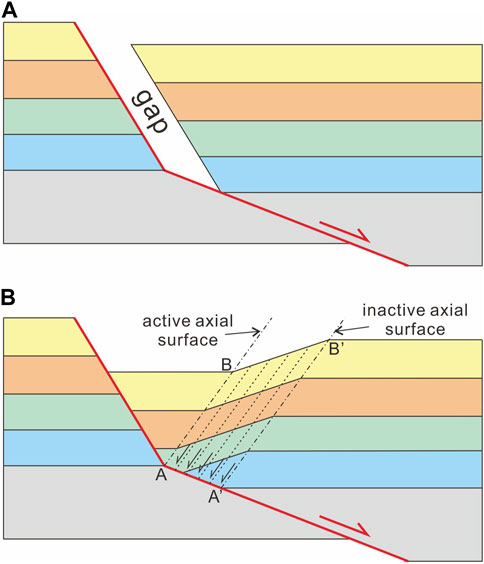
FIGURE 1. A model for a normal fault with a single concave bend. (A) Development of a gap during rightward sliding of hanging wall with high strength. (B) Antithetic simple shear deformation of the hanging wall.
Assuming the presence of a normal fault with a single convex bend, as the hanging wall moves, an overlap region will emerge between the hanging wall and the footwall if the former remains undeformed (Figure 2A). In order to prevent overlap, deformation of the hanging wall is necessary. However, if antithetic normal faulting is applied to convex bends, a reverse shear sense in the hanging wall would be required (Figure 2B), which contradicts the extensional characteristics of the deformation. Therefore, for convex bends, synthetic normal faulting represents a more plausible mechanism for the collapse deformation of the hanging wall (Figure 2C; Xiao and Suppe, 1992).
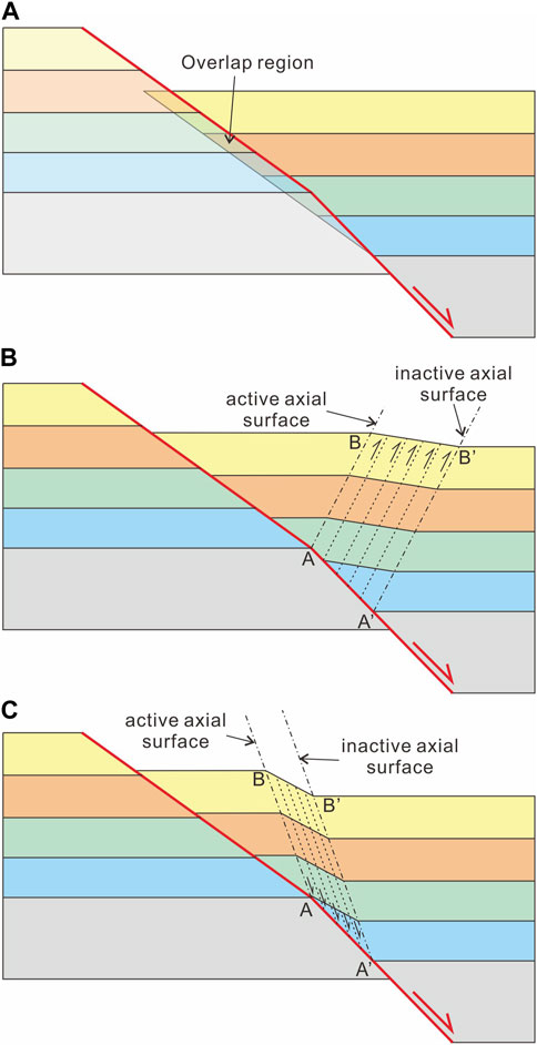
FIGURE 2. A model for a normal fault with a single convex bend. (A) Overlap region development during rightward sliding of hanging wall with undeformed hanging wall. (B) Antithetic simple shear with reverse shear sense applied to the convex bend, contradicting the extensional characteristics of the deformation. (C) Synthetic simple shear with normal shear sense indicates a more plausible mechanism for the convex bend.
3 Results
3.1 Fault slip rates calculation with one fault bend
3.1.1 Concave fault bend
Consider the simple case of one concave fault bend, as shown in Figure 3. The angle
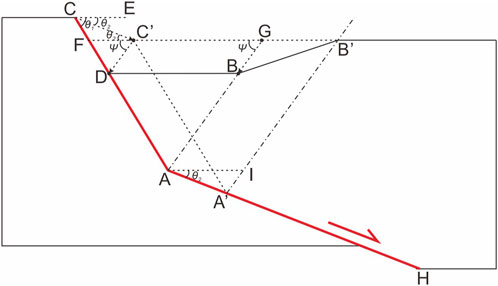
FIGURE 3. Geometric schematic diagram used in deriving the relationship between the slip rates of the upper and lower fault segments with a single concave bend.
If the hanging wall undergoes a displacement AA′ along the lower fault segment, the position of point C will be relocated to point C′. Thus, we have
Throughout the deformation of the hanging wall, the displacement of point C′ results in its relocation to point D, while the displacement of point G leads to its relocation to point B. Thus, we have
Applying the law of sines to ∆CDC′, we have
If we only know the displacement of slip along the upper segment of the fault CD. Given the knowledge of the duration of fault slip, we obtain
where
where
3.1.2 Convex fault bend
Consider the simple case of one convex fault bend, as shown in Figure 4. The angle
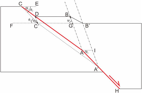
FIGURE 4. Geometric schematic diagram used in deriving the relationship between the slip rates of the upper and lower fault segments with a single convex bend.
If the hanging wall undergoes a displacement AA′ along the lower fault segment, the position of point C will be relocated to point C′. Thus, we have
Throughout the deformation of the hanging wall, the displacement of point C’ results in its relocation to point D, while the displacement of point G leads to its relocation to point B. Thus, we have
Applying the law of sines to ∆CDC′, we have
In the majority of cases, we only know the displacement of slip along the upper segment of the fault CD. Given the knowledge of the duration of fault slip, we obtain
where
Combining Eqs 18, 19, we obtain
where
3.2 Fault slip rates calculation with multiple fault bends
Now that we have established the slip rate law for a fault with a single fault bend, we shall proceed to investigate the slip rate law for faults with multiple fault bends. In the case of continuously curved listric normal faults, we can treat them as a large number of fault bends between arbitrarily small, straight, fault segments.
Consider a fault with one concave fault bend and one convex fault bend, as depicted in Figure 5A. The dip of the upper fault segment is
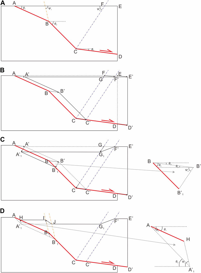
FIGURE 5. Geometric schematic diagram used in deriving the relationship between the slip rates of different fault segments with multiple fault bends. (A) Initial state of a fault with a concave bend and a convex bend. (B) The hanging wall slips along the lower fault segment with a displacement of CC’ during the first stage. (C) The polygon A’B’C’F’ of the hanging wall deforms to form the polygon A1′B1’CC’F’G1 during the second stage. (D) The polygon A1′B1’CC’F’G1 deforms to form the polygon HBCC’F’G1JI during the final stage.
For the convenience of calculation, we partition the deformation into three steps.
Firstly, the hanging wall undergoes displacement CC’ along the lower fault segment. Consequently, points A, B, C, D, E, and F move to points A′, B′, C′, D′, E′, and F′, respectively (Figure 5B). Thus, we have
Secondly, the collapse deformation of the polygon A’B’C’F’ of the hanging wall forms the polygon A1′B1’CC’F’G1 (Figure 5C). Applying the law of sines to ∆BB′B′1, we have
Finally, the polygon A1′B1′CC′F′G1 undergoes deformation to form the polygon HBCC′F′G1JI (Figure 5D). Applying the law of sines to ∆AHA′1, we have
Based on the aforementioned analysis, it can be readily inferred that the displacement relationship on both sides of a fault bend is solely determined by the type of bend (concave or convex), the individual dip angles of the respective fault segments, and the dip angle of the axial surface at the bend, independent of other factors.
Therefore, for a fault with n segments and n-1 bends, the following relationships hold:
where
Based on Eqs 26, 27, if the dip angles of each fault segment, the properties of each fault bend, the dip angles of each axial surface, and the displacement on one of the fault segments are known, then the displacements on the remaining fault segments can be derived. Furthermore, if the duration of motion is also known, the slip rates on each segment can be obtained.
It is noteworthy that if each bend in the fault is either convex or concave in shape, and the dip angles of the axial surfaces are identical, the following relationships hold:
where
Eqs 28, 29 indicate that if the dip angle of the axial surface and the displacement on one of the fault segments are known, determining the displacement on another fault segment only requires knowledge of its corresponding dip angle. This implies that once the dip angles of two fault segments are determined, regardless of the number of intervening fault segments or their dip angles, it will not alter the relationship between the displacements of these two fault segments.
This conclusion is highly useful because in most cases, bends of listric normal faults tend to be concave in shape. If the mechanical properties of the hanging wall are similar, the dip angle of the axial surface remains relatively constant. So even if we only have access to fault displacements and rates at the surface or shallow depths, we can infer the displacements and slip rates along the deeper fault segments. Furthermore, the horizontal extension rate can be inferred since listric normal faults tend to flatten at depth:
where
3.3 Long slip distance of faults
Previously, we only discussed the case where the slip distance was limited to a small segment of the fault. Now, we will analyze the scenario where the slip distance is longer and spans across multiple fault segments.
Consider a fault with three concave fault bends, as depicted in Figure 6A. The dip of the fault segment AB is
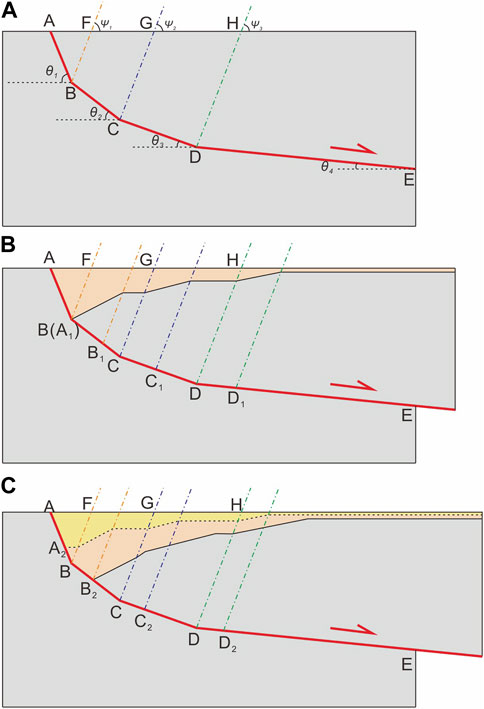
FIGURE 6. A geometric model with three concave bends used in deriving the relationship between slip rates at shallow and deep depths when the slip distance is long. (A) Initial state of a fault with three concave bends. (B) Orange growth strata deposit as the hanging wall slips along the DE segment with a displacement of DD1 during the first stage. (C) Yellow growth strata deposit as the hanging wall slips along the DE segment with a displacement of DD2 during the second stage.
If Figure 6C represents the final state after deformation, the deformation process can be divided into two stages. During the first stage, the hanging wall slides a distance of DD1 along the DE segment. At this point, the sliding distance along the AB segment is AA1 (Figure 6B). Based on the Eqs 26, 27, we have
Combining Eqs 31–33, we obtain the relationship between AB and DD1:
Subsequently, the hanging wall slides a distance of DD2 along the DE segment, while the sliding distance along the AB segment is AA2 (Figure 6C). Based on the Eqs 26, 27, we have
Combining (Eqs 36, 37), we obtain the relationship between BB2 and DD2:
If we know the lengths of AB and BB1 in the final state, as well as the duration of time elapsed from the initial state to the final state, we can obtain the fault slip rate along the DE segment during this time period by utilizing (Eqs 34, 38):
where
If the dip angles of axial surfaces are equal to
If orange and yellow growth strata were sequentially deposited during the first and second stages of fault slip, it may be feasible to deduce the duration of each stage (Figure 6C). This information can be used to determine the slip rate of the fault along segment DE for each stage period:
where
If the dip angles of axial surfaces are equal to
4 Geological example
A seismic section from the Bohai Bay Basin is presented as an illustrative example of how slip rates at various depths during different time intervals are calculated (Figure 7). In the seismic section, the Chengnan Fault is identified as a listric normal fault characterized by a combination of concave and convex bends. During the Paleogene period, the Bohai Bay Basin underwent substantial extensional tectonics, leading to pronounced activity along the Chengnan Fault within this geological epoch (Qi and Yang, 2010; Li et al., 2012; Zhao et al., 2016). Three sequences of growth strata (Growth Strata 1, Growth Strata 2, Growth Strata 3) were deposited on the hanging wall of the fault, each delimited by reflection boundaries T1, T2, T6, and Tr. The corresponding ages for these reflection boundaries are 24.6 Ma, 33 Ma, 43.5 Ma, and 65 Ma, respectively (Ren, 2004; Yao et al., 2007a; Yao et al., 2007b). Growth strata 1 is constrained by seismic reflection boundaries T1 and T2, indicating sedimentation occurred between 24.6 Ma and 33 Ma. Growth strata 2 is defined by seismic reflection boundaries T2 and T6, suggesting sedimentation took place between 33 Ma and 43.5 Ma. Lastly, Growth strata 3 is delimited by seismic reflection boundaries T6 and Tr, indicating sedimentation occurred between 43.5 Ma and 65 Ma. In the following, the calculation of slip rates for the Chengnan Fault at various depths during the intervals of 24.6–33 Ma, 33–43.5 Ma, and 43.5–65 Ma are estimated.
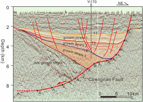
FIGURE 7. Seismic section of a listric normal fault from the Bohai Bay Basin characterized by a combination of concave and convex bends.
Initially, it is necessary to replace the curved Chengnan Fault with multiple straight segments (from A1A2 to A16A17) and measure the dip angle of each segment (Table 1). It is worth noting that to calculate the true dip angle of the fault, it is necessary to adjust the lateral and vertical scales of the seismic profile to be consistent.
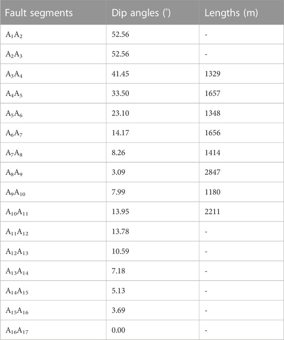
TABLE 1. Dip angles and lengths of each fault segment.
Subsequently, the lengths of the fault segments involved in the growth strata (from A3A4 to A10A11) are measured (Table 1). Utilizing Eqs 26, 27 to convert the lengths of segments from A3A4 to A10A11 into lengths at different dip angles (Table 2). For example, the length of segment A3A4 is 1329 m, with a dip angle of 41.45°. When converted to a dip angle of 52.56°, which is the angle for segment A2A3, the length becomes 1410 m.
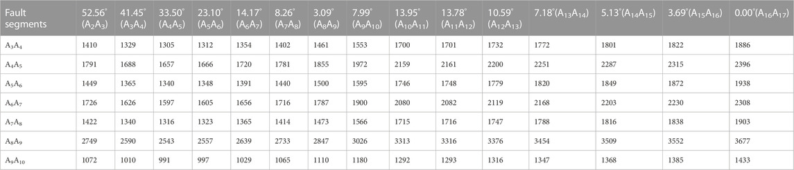
TABLE 2. Conversion of lengths of segments A3A4 to A10A11 into lengths at different dip angles (m).
Finally, sum the results of the converted segments involved in different time intervals and divide by the time intervals to obtain the slip rates of the Chengnan Fault at different fault segments, or different depths, during different time periods. For instance, during the deposition of Growth Strata 2, which corresponds to the time interval of 33–43.5 Ma, the fault segments involved are A4A5, A5A6, and A6A7. To determine the slip rate of the fault at segment A2A3 during the 33–43.5 Ma period, the lengths of A4A5, A5A6, and A6A7 are converted to a 52.56° dip angle, resulting in lengths of 1791m, 1449m, and 1726m, respectively. These lengths are then summed to obtain 4966 m and divided by the time interval of 10.5 Ma, resulting in a calculated slip rate of 473 m/Ma. The slip rate results for each fault segment within the three time intervals: 24.6–33 Ma, 33–43.5 Ma, and 43.5–65 Ma, are presented in Table 3; Figure 8.
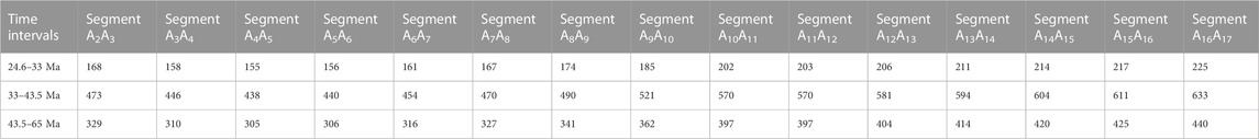
TABLE 3. Slip rates of the Chengnan fault at various segments during three time intervals: 24.6–33 Ma, 33–43.5 Ma, and 43.5–65 Ma (m/Ma).
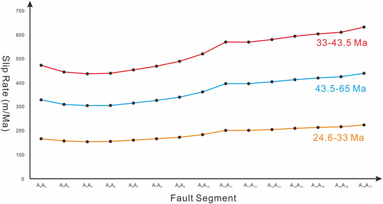
FIGURE 8. Line plot of fault slip rates along segments of the Chengnan Fault during the periods 24.6–33 Ma, 33–43.5 Ma, and 43.5–65 Ma.
From Figure 8, it can be observed that the fault slip rate along the Chengnan Fault decreases gradually from segment A2A3 to A4A5. However, from segment A4A5 onwards and all the way to segment A16A17, the slip rate gradually increases. The maximum slip rate occurs at segment A16A17, while the minimum is observed at segment A4A5, resulting in a ratio of 1.45 between the two. The following discussion section will analyze the patterns of slip rate variations along different segments.
5 Discussion
5.1 Concave fault bend
For a fault with only one concave fault bend, the relationship between the slip rates along the upper segment and the lower segment can be determined based on Equation 10:
where
Previous studies have suggested that the angle
Figure 9 depicts the values of
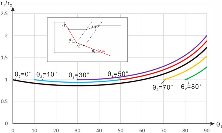
FIGURE 9. Graph of relationships between the value of
Furthermore, it can be observed that as the value of
The above analysis reveals that, in most cases, the slip rates on different segments of a listric normal fault are not equal. If the surface or shallow segments of the listric normal fault exhibit a large dip angle, the slip rate along these segments is often greater than that of the deeper segments, with a maximum ratio of two times. For the listric normal fault, as it tends to be nearly horizontal at greater depths, the slip rate obtained on the shallow fault segment with a large dip angle is generally larger than that at deeper depths, potentially up to twice as large. It should be noted that listric normal faults may also exhibit flexure at the kilometer scale due to the rheology of the crust. However, due to the limited variation in dip angles, the impact on fault slip rates can be considered negligible according to Eq. 45.
Conversely, if the surface or shallow segments of the listric normal fault have a small dip angle, the slip rate along these segments tends to be smaller than that of the deeper segments, but the difference between the two is relatively close. In the latter case, the minimum ratio is approximately 0.866 times that of the deeper segments.
Another noteworthy observation is that for two faults with the same dip angle in the deep segment, even if their actual slip distances at depth are equal, significant differences in the displacement exhibited in the shallow segment can arise if the dip angles of the shallow segments are different.
For instance, consider fault ABC and fault A′B′C′, where the dip angles of segments BC and B′C′ are both 0°, the dip angle of segment AB is 30°, and the dip angle of segment A′B′ is 80° (Figure 10). Assuming the axial surface orientation of 60°, if the hanging wall undergoes a horizontal slip distance of x, the displacement AD in the shallow segment of fault ABC is 0.87x, while the displacement A′D′ in the shallow segment of fault A′B′C′ is 1.35x. Based on the results obtained from the shallow segments, one might conclude that fault A′B′C′ exhibits greater activity than fault ABC. However, this conclusion is erroneous when considering the deep segments.

FIGURE 10. Comparative diagram of concave normal faults with equal extensional rates but varied dip angles of upper segment. (A) A concave normal fault model with 30° dip of upper segment. (B) A concave normal fault model with 80° dip of upper segment.
Furthermore, if one were to infer the regional horizontal extension based on the calculation of horizontal displacement in the shallow segment of the fault, it would result in conclusions that deviate from the actual scenario. The horizontal displacement of AD measures 0.75x, while the horizontal displacement of A′D′ amounts to 0.23x. Based on these values, one might perceive fault ABC to have a greater extension rate compared to fault A′B′C′. However, in reality, both faults exhibit equal extension rates.
When there is deposition of growth strata, previous researches (Huang et al., 2014; Zhang et al., 2020) attempt to estimate the strength of tectonic extension based on the thickness of the growth strata. However, such an approach sometimes is problematic. For fault ABC, the thickness of the growth strata, which is equivalent to the vertical displacement AD, is 0.43x. For fault A′B′C′, the thickness of the growth strata, equivalent to the vertical displacement A′D′, is 1.33x. Based on the thickness of the growth strata, fault A′B′C′ appears to exhibit a stronger tectonic extension than fault ABC. Nevertheless, in reality, the extension rates of these two faults are equal because BE is equal to B′E′.
5.2 Convex fault bend
For a fault with only one convex fault bend, the relationship between the slip rates along the upper segment and the lower segment can be determined based on Eq. 11:
where
Similarly, we take
Figure 11 depicts the values of
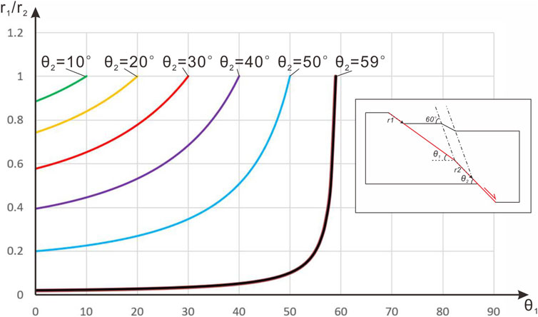
FIGURE 11. Graph of relationships between the value of
It is noteworthy that when
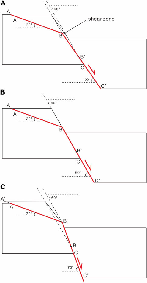
FIGURE 12. Models of convex normal faults with high dip angles of the lower segment. (A) A convex normal fault model with 55° dip of lower segment. (B) A convex normal fault model with 60° dip of lower segment. (C) A convex normal fault model with 70° dip of lower segment.
When
This model is incapable of predicting scenarios where
6 Conclusion
The study derived relationships between fault slip rates at different depths based on the inclined shear model. The following conclusions were obtained:
(1) For the listric normal fault, if the fault dip angles differ at two different depths, their slip rates generally vary. The extent of variation primarily depends on the fault dip angles at the respective depths, the type of fault bend, and the dips of the axial surfaces.
(2) In the case of a concave fault bend, when the dip of the lower fault segment is between 0° and 30°, the ratio of slip rates between the upper and lower segments initially decreases with an increase in the dip of the upper fault segment. Subsequently, the ratio increases with an increase in the dip of the upper fault segment, but the magnitude of decrease is not as significant as the magnitude of increase. If the dip of the lower fault segment exceeds 30°, the ratio of slip rates between the upper and lower segments continually increases with an increase in the dip of the upper fault segment.
(3) For a convex fault bend, regardless of the dip of the lower fault segment, the ratio of slip rates between the upper and lower segments continually decreases with an increase in the dip of the upper fault segment.
(4) For the listric normal fault, as it tends to be nearly horizontal at greater depths, the slip rate obtained on the shallow fault segment with a large dip angle is generally larger than that at deeper depths, potentially up to twice as large. Conversely, if the shallow fault segment has a small dip angle, the slip rate obtained there is slightly smaller than that at deeper depths.
(5) Based on the dip-slip and horizontal displacement of shallow faults, as well as the thickness of the growth strata, to infer the strength of regional horizontal extension is prone to yielding erroneous conclusions. To achieve a more accurate assessment, a comprehensive analysis integrating the geometric configuration of the fault and deformation pattern of the hanging wall is necessary.
(6) Between 24.6 and 33 Ma, the Chengnan Fault exhibited slip rates of 155–206 m/Ma, which increased to 438–581 m/Ma from 33 to 43.5 Ma, and subsequently remained in the range of 305–404 m/Ma from 43.5 to 65 Ma. The calculation of slip rates for the Chengnan Fault at various depths indicates a decreasing trend from segment A2A3 to segment A4A5, followed by an increasing trend from segment A4A5 to segment A16A17.
Data availability statement
The original contributions presented in the study are included in the article/supplementary material, further inquiries can be directed to the corresponding author.
Author contributions
YZ: Conceptualization, Data curation, Formal Analysis, Funding acquisition, Investigation, Methodology, Project administration, Resources, Software, Supervision, Validation, Visualization, Writing–original draft, Writing–review and editing.
Funding
The author declares financial support was received for the research, authorship, and/or publication of this article. This research has received financial support from the research initiation fund of Zhejiang University of Water Resources and Electric Power.
Acknowledgments
I would like to express my gratitude to Professor Hanlin Chen and Professor Fengqi Zhang for providing the seismic section and guidance in the interpretation. I am also thankful for the valuable comments and suggestions from three reviewers, which greatly contributed to this paper.
Conflict of interest
The author declares that the research was conducted in the absence of any commercial or financial relationships that could be construed as a potential conflict of interest.
Publisher’s note
All claims expressed in this article are solely those of the authors and do not necessarily represent those of their affiliated organizations, or those of the publisher, the editors and the reviewers. Any product that may be evaluated in this article, or claim that may be made by its manufacturer, is not guaranteed or endorsed by the publisher.
References
Anderson, J. G., Wesnousky, S. G., and Stirling, M. W. (1996). Earthquake size as a function of fault slip rate. Bull. Seismol. Soc. Am. 86, 683–690. doi:10.1785/BSSA0860030683
Benedetti, L., Finkel, R., Papanastassiou, D., King, G., Armijo, R., Ryerson, F., et al. (2002). Post-glacial slip history of the Sparta fault (Greece) determined by 36Cl cosmogenic dating: evidence for non-periodic earthquakes. Geophys. Res. Lett. 29, 1246. doi:10.1029/2001GL014510
Blakeslee, M. W., and Kattenhorn, S. A. (2013). Revised earthquake hazard of the Hat Creek fault, northern California: a case example of a normal fault dissecting variable-age basaltic lavas. Geosphere 9, 1397–1409. doi:10.1130/GES00910.1
Bull, J. M., Barnes, P. M., Lamarche, G., Sanderson, D. J., Cowie, P. A., Taylor, S. K., et al. (2006). High-resolution record of displacement accumulation on an active normal fault: implications for models of slip accumulation during repeated earthquakes. J. Struct. Geol. 28, 1146–1166. doi:10.1016/j.jsg.2006.03.006
Dula, W. F. (1991). Geometric models of listric normal faults and rollover folds. AAPG Bull. 75, 1609–1625. doi:10.1306/0C9B29B1-1710-11D7-8645000102C1865D
Friedrich, A. M., Wernicke, B. P., Niemi, N. A., Bennett, R. A., and Davis, J. L. (2003). Comparison of geodetic and geologic data from the Wasatch region, Utah, and implications for the spectral character of Earth deformation at periods of 10 to 10 million years. J. Geophys. Res. Solid Earth 108, 2199. doi:10.1029/2001JB000682
Galadini, F., and Galli, P. (2000). Active tectonics in the central Apennines (Italy) - input data for seismic hazard assessment. Nat. Hazards 22, 225–270. doi:10.1023/A:1008149531980
Groshong, R. H. (1989). Half-graben structures: balanced models of extensional fault-bend folds. Geol. Soc. Am. Bull. 101, 96–105. doi:10.1130/0016-7606(1989)101<0096:HGSBMO>2.3.CO;2
Hauge, T. A., and Gray, G. G. (1996). A critique of techniques for modelling normal-fault and rollover geometries. Geol. Soc. Lond. Spec. Publ. 99, 89–97. doi:10.1144/gsl.sp.1996.099.01.08
Huang, L., Liu, C. Y., Wang, Y., Zhao, J., and Mountney, N. P. (2014). Neogene-Quaternary postrift tectonic reactivation of the Bohai Bay Basin, eastern China. AAPG Bull. 98, 1377–1400. doi:10.1306/03071413046
Kerr, H. G., and White, N. (1992). Laboratory testing of an automatic method for determining normal fault geometry at depth. J. Struct. Geol. 14, 873–885. doi:10.1016/0191-8141(92)90047-Z
Li, S., Zhao, G., Dai, L., Zhou, L., Liu, X., Suo, Y., et al. (2012). Cenozoic faulting of the Bohai Bay Basin and its bearing on the destruction of the eastern north China craton. J. Asian Earth Sci. 47, 80–93. doi:10.1016/j.jseaes.2011.06.011
McClymont, A. F., Villamor, P., and Green, A. G. (2009). Fault displacement accumulation and slip rate variability within the Taupo Rift (NewZealand) based on trench and 3-D ground-penetrating radar data. Tectonics 28, TC4005. doi:10.1029/2008TC002334
Mitchell, S. G., Matmon, A., Bierman, P. R., Enzel, Y., Caffee, M., and Rizzo, D. (2001). Displacement history of a limestone normal fault scarp, northern Israel, from cosmogenic 36Cl. J. Geophys. Res. Solid Earth 106, 4247–4264. doi:10.1029/2000JB900373
Mouslopoulou, V., Walsh, J. J., and Nicol, A. (2009). Fault displacement rates on a range of timescales. Earth Planet. Sci. Lett. 278, 186–197. doi:10.1016/j.epsl.2008.11.031
Nicol, A., Walsh, J., Berryman, K., and Villamor, P. (2006). Interdependence of fault displacement rates and paleoearthquakes in an active rift. Geology 34, 865–868. doi:10.1130/G22335.1
Nicol, A., Walsh, J., Watterson, J., and Underhill, J. R. (1997). Displacement rates of normal faults. Nature 390, 157–159. doi:10.1038/36548
Nicol, A., Walsh, J. J., Manzocchi, T., and Morewood, N. (2005). Displacement rates and average earthquake recurrence intervals on normal faults. J. Struct. Geol. 27, 541–551. doi:10.1016/j.jsg.2004.10.009
Nicol, A., Walsh, J. J., Villamor, P., Seebeck, H., and Berryman, K. R. (2010). Normal fault interactions, paleoearthquakes and growth in an active rift. J. Struct. Geol. 32, 1101–1113. doi:10.1016/j.jsg.2010.06.018
Qi, J., and Yang, Q. (2010). Cenozoic structural deformation and dynamic processes of the Bohai Bay basin province, China. Mar. Petroleum Geol. 27, 757–771. doi:10.1016/j.marpetgeo.2009.08.012
Ren, J. (2004). Tectonic significance of S6’ boundary in dongying depression, Bohai gulf basin. Earth Science-Journal China Univ. Geosciences 29, 69–82. doi:10.3321/j.issn:1000-2383.2004.01.013
Schlagenhauf, A., Gaudemer, Y., Benedetti, L., Manighetti, I., Palumbo, L., Schimmelpfennig, I., et al. (2010). Using in situ Chlorine-36 cosmonuclide to recover past earthquake histories on limestone normal fault scarps: a reappraisal of methodology and interpretations. Geophys. J. Int. 182, 36–72. doi:10.1111/j.1365-246X.2010.04622.x
Schlagenhauf, A., Manighetti, I., Benedetti, L., Gaudemer, Y., Finkel, R., Malavieille, J., et al. (2011). Earthquake supercycles in central Italy inferred from 36Cl exposure dating. Earth Planet. Sci. Lett. 307, 487–500. doi:10.1016/j.epsl.2011.05.022
White, N. (1992). A method for automatically determining normal fault geometry at depth. J. Geophys. Res. Solid Earth 97, 1715–1733. doi:10.1029/91JB02565
White, N., and Yielding, G. (1991). Calculating normal fault geometries at depth: theory and examples. Geol. Soc. Lond. Spec. Publ. 56, 251–260. doi:10.1144/gsl.sp.1991.056.01.18
White, N. J., Jackson, J. A., and McKenzie, D. P. (1986). The relationship between the geometry of normal faults and that of the sedimentary layers in their hanging walls. J. Struct. Geol. 8, 897–909. doi:10.1016/0191-8141(86)90035-0
Withjack, M. O., Islam, Q. T., and La Pointe, P. R. (1995). Normal faults and their hanging-wall deformation: an experimental study. AAPG Bull. 79, 1–17. doi:10.1306/8D2B1494-171E-11D7-8645000102C1865D
Withjack, M. O., and Peterson, E. T. (1993). Prediction of normal-fault geometries—a sensitivity analysis. AAPG Bull. 77, 1860–1873. doi:10.1306/BDFF8F60-1718-11D7-8645000102C1865D
Withjack, M. O., and Schlische, R. W. (2006). Geometric and experimental models of extensional fault-bend folds. Geol. Soc. Lond. Spec. Publ. 253, 285–305. doi:10.1144/GSL.SP.2006.253.01.15
Xiao, H., and Suppe, J. (1992). Origin of rollover. AAPG Bull. 76, 509–529. doi:10.1306/BDFF8858-1718-11D7-8645000102C1865D
Yao, Y., Xu, D., Han, Y., Yin, Z., and Zhang, H. (2007a). Astrostratigraphic age analysis of the eocene–oligocene boundary in the jiyang depression, shandong. J. Stratigr. 31, 483–494. doi:10.19839/j.cnki.dcxzz.2007.s2.008
Yao, Y., Xu, D., Zhang, H., Han, Y., Zhang, S., Yin, Z., et al. (2007b). A brief introduction to the Cenozoic astrostratigraphic time scale for the Dongying Sag, Shandong. J. Stratigr. 31, 423–429. doi:10.19839/j.cnki.dcxzz.2007.s2.002
Youngs, R. R., and Coppersmith, K. J. (1985). Implications of fault slip rates and earthquake recurrence models to probabilistic seismic hazard estimates. Bull. Seismol. Soc. Am. 75, 939–964. doi:10.1785/BSSA0750040939
Zhang, Y., Dilek, Y., Zhang, F. Q., Chen, H. L., Zhu, C. T., and Hao, X. F. (2020). Structural architecture and tectonic evolution of the cenozoic zhanhua sag along the tan-Lu fault zone in the eastern north China: reconciliation of tectonic models on the origin of the Bohai Bay Basin. Tectonophysics 775, 228303. doi:10.1016/j.tecto.2019.228303
Keywords: fault slip rate, listric normal fault, concave bend, convex bend, extensional rate
Citation: Zhang Y (2023) A geometric analysis of slip rate variation with depth in listric normal faults. Front. Earth Sci. 11:1266454. doi: 10.3389/feart.2023.1266454
Received: 25 July 2023; Accepted: 20 November 2023;
Published: 29 December 2023.
Edited by:
James D. Muirhead, The University of Auckland, New ZealandReviewed by:
Bhaskar Kundu, National Institute of Technology Rourkela, IndiaR. Jayangonda Perumal, Wadia Institute of Himalayan Geology, India
Alexis Rigo, UMR8538 Laboratoire de Géologie de l'Ecole Normale Supérieure (LG-ENS), France
Copyright © 2023 Zhang. This is an open-access article distributed under the terms of the Creative Commons Attribution License (CC BY). The use, distribution or reproduction in other forums is permitted, provided the original author(s) and the copyright owner(s) are credited and that the original publication in this journal is cited, in accordance with accepted academic practice. No use, distribution or reproduction is permitted which does not comply with these terms.
*Correspondence: Yao Zhang, Mjc5ODkzNzYwQHFxLmNvbQ==