Full waveform inversion with combined misfit functions and application in land seismic data

Full waveform inversion reconstructs subsurface structures by matching the synthetic waveform to the observed waveform. Inaccuracy of the source wavelets can, thus, easily lead to an inaccurate model. Simultaneously updating source wavelets and model parameters is a conventionally used strategy. However, when the initial model is very far from the true model, cycle skipping exists, and estimating a reliable source wavelet is very difficult. We propose a combinatory inversion workflow based on seismic events. We apply a Gaussian time window around the first break and gradually increase its width to include more seismic events. The influence of inaccurate source wavelets is alleviated by applying a Gaussian time window around the first break to evaluate the normalized cross-correlation-based objective function. There are inevitable small model artifacts caused by inter-event interactions when calculating cross-correlations. As a result, we switch to the optimal transport function to clean the model and update the source wavelets simultaneously. The combinatory strategy has been applied to models with different types of geological structures. Starting from a crude initial model, we recovered a high-resolution and high-fidelity model and the source wavelets in two synthetic experiments. Finally, we apply our inversion strategy to a real-land seismic dataset in Southeast China and obtain a higher-resolution velocity model. By comparing an inversion velocity profile with well log information and the recorded data with the simulated data, we conclude that our inversion results for the field data are accurate and this new strategy is effective.

1 Introduction

Full waveform inversion (FWI) aims to reconstruct a high-resolution (fine structures are revealed), high-fidelity (structures are real) subsurface model by fitting the synthetics to the observed seismic data (Lailly, 1983; Tarantola, 1984). FWI starts from an initial model, measures the waveform difference between simulated and observed data, and accordingly modifies the model to decrease the difference. In the end, not only the phases of the seismograms but also the amplitudes are fully fitted. It is the most powerful imaging tool (Virieux and Operto, 2009; Alkhalifah, 2016). Since seismic signals are highly oscillating, FWI may encounter cycle skipping and become trapped into local minima. A sufficiently accurate initial model is usually necessary (Gauthier et al., 1986). The cycle-skipping issue is severe when an accurate source wavelet is not available. In this study, we investigate this issue of a crude initial model and unavailable true source wavelet.

The earliest objective function of FWI is the conventional least-squares (L2) function. L2 compares the synthetic event to the nearest phase in the observed seismograms. It requires a sufficiently accurate initial model to ensure that the main synthetic events are within the half period. Otherwise, the seismic events could be wrongly interpreted as other phases. Increasing the length of the periods so that the seismic signals are less oscillating is one immediate solution. Bunks et al. (1995) progressively filtered seismograms from the low-frequency band to the high-frequency band. The inverted model is taken as the initial model for the next frequency band until the entire available frequencies are exploited. This frequency continuation inversion strategy could perform better when specific phases are selected with time windows (Shipp and Singh, 2002; Brossier et al., 2009b; Wang and Rao, 2009; Wang et al., 2014). Diving waves are selected to reconstruct long-wavelength macro-model structures. Then, expanding or removing the time window at later stages to include reflections allows us to reconstruct finer and deeper structures. Another attempt to alleviate the cycle-skipping problem is to decompose the gradient (Li et al., 2022).

The least-squares objective function, along with the hierarchical inversion strategies, does not fully avoid the local minima. Efforts have been made to seek objective functions with wider basins of attraction (Huber, 1973; Bube and Langan, 1997; Guitton and Symes, 2003; Shin and Ha, 2008; Brossier et al., 2009a; Ha et al., 2009; Alkhalifah and Choi, 2014; Huang, 2014; Warner and Guasch, 2014; Sun and Alkhalifah, 2019a). These objective functions either decrease the oscillation of the seismic traces or place more weight on the phases of seismic events than amplitudes. The L1 norm function [least absolute value; (Claerbout and Muir, 1973; Tarantola, 1987)] is less sensitive to noise than L2, as demonstrated by Brossier et al. (2010) using the onshore SEG/EAGE overthrust model. The envelope of a seismic trace is also less oscillatory than that of the original seismic trace. Luo and Wu (2015) showed the advantage of the envelope function (Bozdağ et al., 2011; Chi et al., 2014; Wu et al., 2014; Song et al., 2019) over the conventional L2 function with the Marmousi model. The wavelet transform has also been used to decrease the oscillating nature of the seismic trace (Yuan and Simons, 2014). The zero-lag cross-correlation function (Routh et al., 2011a,b; Dutta et al., 2014; Liu et al., 2017; Tao et al., 2017) reduces the amplitude information and allows for a slightly incorrect source wavelet (Liu et al., 2017); nevertheless, the initial model should be accurate. Recently, the optimal transport (OT)-based objective function [OT objective function; Engquist and Froese (2014); Engquist et al. (2016); Métivier et al. (2016a); Métivier et al. (2016b); Sun and Alkhalifah (2019b); Yang et al. (2018); Yong et al. (2019a,b)] has been introduced from image processing (Ferradans et al., 2014; Lellmann et al., 2014) to exploration geophysics. The OT algorithm also decreases the role of amplitudes of seismic events, and an OT adjoint source is less oscillating than the synthetics or observed data. Métivier et al. (2016a) successfully recovered various classical seismic models and interpreted the Chevron 2014 blind test.

The travel time-based objective function expands the basin of attraction. FWI under this function is also known as wave-equation tomography [WET; (Luo and Schuster, 1991; Woodward, 1992; Hörmann and De Hoop, 2002; Pratt, 2004; Maarten and van Der Hilst, 2005; Djebbi and Alkhalifah, 2014; Wang et al., 2015)]. The travel time difference, instead of being manually picked, is estimated from the cross-correlation function. The basin of attraction of WET is as broad as ray tracing tomography, but the resolution of WET is higher than that of ray tracing tomography. Wang et al. (2014) conducted a synthetic inversion experiment. The inverted model of ray tracing tomography is not sufficient for following FWI, while the combination of WET and FWI produces a high-resolution high-fidelity model. It is important to select coherent events with an elaborate time window, such as synthetic diving and observed diving waves, and synthetic and observed reflections. The physical meaning of measuring the travel time difference between different phases is ambiguous. The success of combining WET and FWI may be case-dependent due to three difficulties. First, the basin of attraction of WET is so wide that the resolution of WET may not be sufficient for the following FWI. The second difficulty is the shallow penetration depth of diving waves. When the gradient of the velocity structure is small, the diving waves do not penetrate deep into the Earth. Thus, we do not obtain any model updating at depth. Reflections penetrate deeper subsurface layers than diving waves. However, unlike ray tracing tomography, WET cannot target the reflections when the initial model is too smooth to generate any reflection. Third, an accurate source wavelet is important. An incorrect source wavelet affects the cross-correlation and consequently biases the travel time difference.

An improvement to WET is based on the concept of transfer function (Kennett and Fichtner, 2012) or the annihilator (van Leeuwen and Mulder, 2010; Warner and Guasch, 2014). Instead of only extracting the travel time difference from the cross-correlation, the whole normalized cross-correlation is taken as the objective function (van Leeuwen and Mulder, 2008; Zhang and Wang, 2009; van Leeuwen and Mulder, 2010; Zhang et al., 2019). The maximum of the cross-correlation is weighted toward a zero shift. This normalized cross-correlation function has a basin of attraction as wide as that of WET but is less prone to an inaccurate source wavelet. The cross-correlation of two seismic events usually extends over a time span. The objective function is not zero, however, even when the synthetic trace perfectly matches the observed trace. Luo and Sava (2011) proposed to replace the cross-correlation with deconvolution. The resulting seismic signal becomes compressed. Choi and Alkhalifah (2017) followed the idea and showed the advantage of the deconvolution-based objective function. Furthermore, Warner and Guasch (2014) showed better performance by normalizing the deconvolution function.

If inaccurate source wavelets are provided, the data fitting procedure of FWI eventually transfers the inaccuracy to the model space, leading to model inaccuracies. Pratt (1999) proposed to estimate the source wavelets by calculating the Green function in the provided initial model. Later on, Plessix and Cao (2011) developed a technique called the matching filter technique to estimate the source wavelets on the fly. Thus, it becomes feasible to simultaneously update the source wavelets and model parameters. Since the source wavelets are estimated for a given model, the initial model should be sufficiently accurate to produce acceptable source wavelets. To eliminate the source effects, Choi and Alkhalifah (2011) convolved the synthetics with an observed trace and convolved the observed data with a synthetic trace at the same location. Zhang et al. (2016) modified the procedure by windowing the synthetic or observed trace. As pointed out by Choi and Alkhalifah (2011), the convolution increases the nonlinearity, and a more accurate initial model and more elaborate inversion strategies are required.

In this study, we propose another form of a multi-scale inversion strategy. We choose Gaussian time windows to smoothly incorporate more and more seismic events during the inversion. In the first several stages starting from a crude initial model, we choose the normalized cross-correlation objective function. An initial source wavelet is extracted from long offset records. The Gaussian time window allows the seismic events to be fitted gradually: early events are fitted at first, and then, later events are fitted as the window becomes wider. The severity of the cross-talk between events is alleviated when the Gaussian windows are narrow in the early stages. The wide basin of attraction of the normalized cross-correlation objective function helps with the convergence and is also helpful in recovering long-wavelength model structures. We switch to the OT objective function as the Gaussian time window widens, and a matching filter technique is used to estimate the source wavelets at each iteration.

In the following sections, we present the theory of full waveform inversion and explain three objective functions: L2, normalized cross-correlation, and optimal transport function. We test their behaviors with shifted Ricker wavelets. In Section 3, we use two geological models for synthetic tests, show the difficulty encountered with conventional FWI, and explain how our proposed strategy successfully recovers the models and source wavelets. Real-land data application in Sichuan Basin, Southeast China (Song et al., 2015), is also shown. The discussion is presented in Section 5, and conclusion, in Section 6.

2 Three objective functions of full waveform inversion

Full waveform inversion, mathematically speaking, is a local optimization method constrained by a partial differential equation. A pre-defined measure function is provided to evaluate the difference between synthetic and observed seismic data. The conventional measure function is the least-squares function (L2 function). The proposed inversion workflow involves two objective functions, the normalized cross-correlation function and optimal transport function. The partial differential equation is the elasto-dynamic equation, which takes model parameters as input and output seismograms. In this study, we represent the Earth with an acoustic isotropic medium.

2.1 Least-squares objective function

In classical waveform inversion (Lailly, 1983; Tarantola, 1984; Virieux and Operto, 2009), we estimate the earth parameter, m, by minimizing the data residuals. In a time domain formulation, the classic objective function reads

$J\left(\mathbf{m}\right)=\frac{1}{2}{\displaystyle \sum _{s,r}}{\int }_0^T{\left[W_{s,r}\left(t\right)\left(p_{s,r}\left(t\right)-d_{s,r}\left(t\right)\right)\right]}^2\text{d}t,(1)$

where s is the source index, r is the receiver index, p_s,r is the synthetic trace, d_s,r is the observed data trace, and W_s,r is a time window to potentially select the events of interest. The recording length is T. With long-offset data, this window can, for instance, be used to select only the early arrivals, as explained later. The adjoint source is the partial derivative of the right-hand side in Eq. 1 with respect to the synthetic data:

$s\left(t\right)=W_{s,r}^2\left(t\right)\left(p_{s,r}\left(t\right)-d_{s,r}\left(t\right)\right),(2)$

with s(t) as the adjoint source for the trace indexed by s, r (we omitted the lower index).

Our 2D acoustic forward wave simulator is based on a staggered-grid finite-difference scheme (Virieux, 1986), with a free surface boundary condition on top. FWI is based on a local optimization technique or gradient method to iteratively update the unknown parameters (model and source wavelets). The gradient is computed via the adjoint state method (Liu and Tromp, 2006; Plessix, 2006). Briefly speaking, it usually involves a couple of steps. First, a forward wave propagation is conducted for the given model. The border values and the synthetics are saved either in memory or a disk. Then, the synthetic data are compared to the observed data using a given objective function, producing the misfit and the adjoint source. Finally, the adjoint wave fields are simulated with the adjoint source using an adjoint simulator, while, at the same time, the forward wavefields are reconstructed from the saved border values. The accumulated over time product of the adjoint and the reconstructed forward wavefields provides the gradient.

The gradients, which usually contain numerical artifacts for many reasons, are smoothed with an elliptic Gaussian filter. At the first scale, the standard deviation of the Gaussian smoothing filter is 750 m and the vertical one is 150 m. At the final scale, the standard deviation is 150 m and the vertical one is 30 m. To compensate for the decay of the gradient energy with depth, we multiply the gradient by $\sqrt{z+300}$, where z is the depth in meter. Finally, the minimization of the objective function is performed using an l-BFGS quasi-Newton algorithm (Nocedal, 1980).

2.2 Normalized cross-correlation objective function

For the seismic trace indexed by s, r, we denote $\bar{p}(t)=W_{s,r}(t)p_{s,r}(t)$ and $\bar{d}(t)=W_{s,r}(t)d_{s,r}(t)$. The cross-correlation function between the windowed seismic traces is defined as

$c\left(\tau \right)=\text{xcorr}\left(\bar{p},\bar{d}\right)={\int }_0^T\bar{p}\left(t\right)\bar{d}\left(t-\tau \right)\text{d}t.(3)$

The normalized cross-correlation function is defined based on the aforementioned cross correlation as

$J_c=-\frac{{\int }_{-T}^T{c}^2\left(\tau \right)P\left(\tau \right)\text{d}\tau }{{\int }_{-T}^T{c}^2\left(\tau \right)\text{d}\tau },(4)$

where $P(\tau )=\exp (-\frac{{\tau }^2}{2{\zeta }^2})$ is a Gaussian penalty function. ζ is a user-defined parameter that controls the width (proportional to the standard deviation) of the penalty function. We choose ζ to be 5% of the whole recording length ζ = 0.05T in the following inversions. The minus sign is to transform the equation into a minimization problem. The adjoint source is

$s_c\left(t\right)=\frac{W_{s,r}\left(t\right)}{{\int }_{-T}^T{c}^2\left(\tau \right)\text{d}\tau }{\int }_{-T}^T\left(P\left(\tau \right)-2J_c\right)c\left(\tau \right)\bar{d}\left(t-\tau \right)\text{d}\tau .(5)$

Because of the adjoint state method (Liu and Tromp, 2006; Plessix, 2006), it is very convenient to switch from L2 FWI to FWI with the normalized cross-correlation J_c. In an existing FWI program, only the misfit value and the adjoint source need to be changed.

2.3 Optimal transport objective function

Both L2 and the normalized cross-correlation function J_c are 1D comparisons of the seismic data along the trace. L2 is considered a pixel-by-pixel comparison. The optimal transport, depending on the type, could be 1D or 2D. Its 2D version could exploit the lateral coherency along the receiver axis besides the coherency along the time axis. In this case, the data difference for a shot indexed with s is

$J_t={\displaystyle \underset{{\phi }_s\in {\mathrm{B}\mathrm{L}\mathrm{i}\mathrm{p}}_1}{\max }}{\displaystyle \sum _r}{\int }_0^T{\phi }_s\left(x_r,t\right)W_{s,r}\left(t\right)\delta p_{s,r}\left(t\right)\mathrm{d}t\mathrm{\Delta }{x}_r,(6)$

where Δx_r is the receiver spacing, W_s,r(t) is a weighting function introduced to represent the time-windowing technique, and the signed residual δp_s,r = p_s,r − d_s,r is the difference between synthetic and observed shot gathers. BLip₁ is the space of bounded 1-Lipschitz functions defined in the (x_r, t) shot-gather space (Métivier et al., 2016a; Poncet et al., 2018) by

$\begin{array}{ll}\hfill \forall \left(x_r,t\right):& |{\phi }_s\left(x_r,t\right)|<\lambda ,\hfill \\ \hfill \forall \left(x_r,t\right):& |{\phi }_s\left(x_r+\delta x_r,t\right)-{\phi }_s\left(x_r,t\right)|<\delta x_r,\hfill \\ \hfill & |{\phi }_s\left(x_r,t+\delta t\right)-{\phi }_s\left(x_r,t\right)|<\delta t,\hfill \end{array}(7)$

where λ is a pre-defined constant, δx_r is any positive increment in the spatial direction, and δt is any positive temporal increment. The first inequality ensures that the amplitudes of φ_s are bounded; the last two inequalities prevent abrupt variations. The choice of λ was discussed by He et al. (2018). For the 1D optimal transport function, the constraint along the spatial axis is removed. The maximization problem (Eq. 6) can be solved efficiently through proximal splitting techniques (Métivier et al., 2016b). Once the optimal ${\bar{\phi }}_s(x_r,t)$ is determined, the corresponding adjoint source is simply

$s_t\left(t\right)={\bar{\phi }}_s\left(x_r,t\right)W_{s,r}\left(t\right).(8)$

This is a 2D algorithm, and we repeat it for each shot panel in our following inversion examples. Again, thanks to the adjoint state method (Liu and Tromp, 2006; Plessix, 2006), switching from a least-squares objective function to the OT objective function in an existing FWI code only requires changes in the misfit value and, specifically, in the adjoint source.

A quick way to evaluate an objective function is to observe its behavior with moving Ricker wavelets. Figure 1A shows such a test. A 3-Hz Ricker wavelet centered in the middle is taken as an observed seismic trace. The synthetic trace is a shifted 3-Hz Ricker wavelet. The L2 norm objective function shows two local minima; the valley near the true position is really sharp. This is consistent with the fact that cycle skipping is an issue for the L2 norm, but it can help FWI converge fast and produce a high-resolution model if we start with a model within the basin of attraction. For the normalized cross-correlation function J_c, we choose the penalty function P(τ) with ζ = 0.3T = 1.2 s. In Figure 1A, we re-scaled the range to [0,1]. The misfit curve is similar to the travel time-based objective function. There are no local minima. However, the wide valley suggests that FWI, in this case, will converge to a smoother model. We also show the misfit curve with optimal transport function J_t with the 1D algorithm. There are no local minima, and the basin of attraction is a little bit wider than that of the L2 function. However, if the synthetics is too far from the observed trace, the misfit J_t is flat, indicating that there is no sensitivity to the variation in synthetics (Figure 1B). The adjoint sources under J_c and J_t are also shown (the L2 adjoint source is the direct difference between the synthetics and observed trace; thus, it is omitted). For the J_c function, the position of the adjoint source signal aligns with the synthetic trace. This behavior is similar to that of the travel time-based objective function (Dahlen et al., 2000; Nolet, 2008), where the adjoint source is proportional to the derivative of the synthetics ${\dot{p}}_{s,r}(t)$. For the J_t function, the imprints of the synthetic and observed trace are kept in the adjoint source. However, the adjoint source is less oscillating than the synthetic and the observed trace. This is consistent with the fact that the misfit curve of J_t is more convex than that of the L2 function (Figure 3A).

FIGURE 1

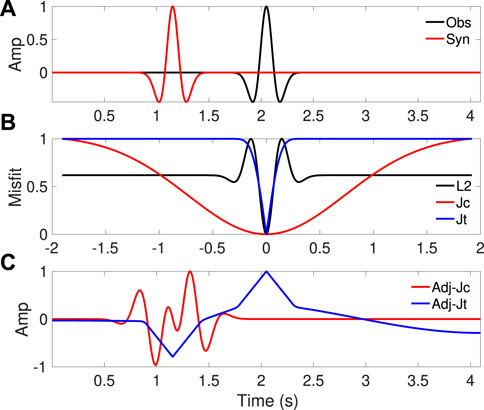
FIGURE 1. Experiment with moving Ricker wavelets to evaluate three objective functions: L2, J_c, and J_t. (A) Top panel shows observed and synthetic traces. (B) Middle panel shows the misfit values. (C) Bottom panel shows the adjoint source of J_c and J_t.

We shift the phase of the synthetics by 90° and calculate the misfit curves and the adjoint sources for these three objective functions in Figure 2. For both the L2 function and J_t function, there are local minima. At the correct travel time t = 0, the misfit values are neither local minima nor local maxima. However, for the J_c objective function, the misfit curve is the same as that shown in Figure 2B. Both of the adjoint sources of J_c and J_t change. The phase shift in the synthetic trace (Figure 2A) is taken into account by the J_c function.

FIGURE 2

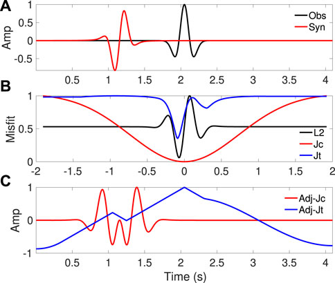
FIGURE 2. Similar experiment and similar labels (A–C) as in Figure 1. However, the synthetic trace is phase shifted by 90°.

3 Combinational strategy for FWI and experimental results

In this section, we explain how we build our inversion workflow. In all our tests, we consider the Middle East model with linearly increasing velocities, and we assume that the true source wavelet is unavailable. First, we show a conventional L2 inversion, where we consider a frequency continuation inversion strategy. In the second inversion experiment, we consider another strategy based on seismic events instead of frequency components. Gaussian windows are applied around the early breaks. The inversion has improved compared to the first experiment. Finally, in the third inversion experiment, we apply our proposed inversion strategy, which yields high-resolution and high-fidelity recovery.

3.1 Middle East model and the observed data

A realistic model mimicking the geology of the Middle East area is taken as the true model. The model contains a succession of shale–sand layers with velocities between 2 and 3.5 km/s, depending on the depth, and carbonate layers with velocities between 3.5 and 6 km/s (Figure 3). Most of the layers have a thickness of several hundred meters.

FIGURE 3

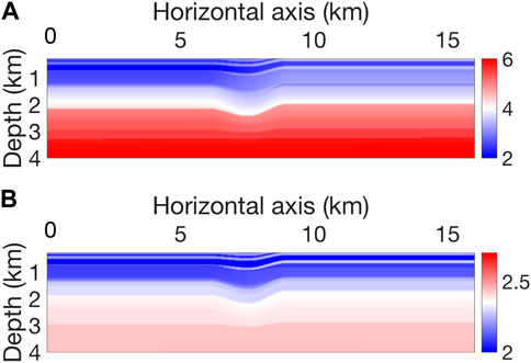
FIGURE 3. (A) True velocity v_p model. (B) True density ρ model. The model contains layered structures and lateral curvatures in the middle.

The acquisition mimics a standard fixed-spread vibroseis acquisition. The observed dataset contains 48 sources, distributed every 300 m, and 300 receivers, spaced every 50 m on the free surface. The observed data are modeled using an acoustic forward operator with a free surface boundary condition. The source wavelet is a 3-Hz Ricker wavelet. The total recording time is 8.192 s. A 1D linearly increasing velocity from 2.2 km/s at the top to 5.5 km/s at the bottom is taken as the initial v_p model (Figure 4). The initial density is linked to the initial v_p model via Gardner’s law (Gardner et al., 1974; Hamilton, 1978). The initial density is overestimated in the deep area.

FIGURE 4

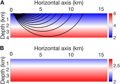
FIGURE 4. (A) The initial velocity v_p is a linearly increasing model. (B) The initial density ρ is calculated from the initial velocity through an empirical relationship, which overestimates the density. Ray trace tomography penetrates deep in this model.

The observed data are shown in Figure 5. The complex observed seismogram contains various waves. Diving waves penetrate deep. Near-offset reflections and inter-bed reflections are due to the lateral layers in the top area. Scattered events are due to the lateral curvature in the middle of the model shown in Figure 3.

FIGURE 5

FIGURE 5. Observed data are calculated with a 3-Hz Ricker wavelet.

3.2 Conventional inversion based on frequency continuation

The conventional inversion is to start from low frequency. We consider the L2 function. The first frequency band is [0.6, 1.5] Hz, which is sufficiently low in typical exploration geophysics. The density is re-calculated from v_p at each iteration via an empirical relationship. By passively updating the density parameter, structural information is introduced from the inverted v_p model to density.

The linearly increasing initial model is too far from the true model. Therefore, when estimating the source wavelets in the initial model, the initial estimated source wavelet is completely different from the true source wavelet: its amplitude is 1,000 times smaller, although the frequency band is more or less consistent. Consequently, l-BFGS only updated the model for two iterations before having difficulty determining a suitable step length. The final model is almost identical to the initial model. We do not move to a higher-frequency band. Our rationale is that if the inversion is trapped in a local minimum at low frequency, moving to high frequency induces more local minima.

We replace the L2 function with OT objective function and repeat the inversion in this low-frequency band [0.6, 1.5] Hz. Nevertheless, a similar phenomenon is observed, probably because the estimated source wavelet is very far from the true source wavelet.

3.3 Inversion strategy based on Gaussian time windows

Instead of a frequency continuation strategy, we can also consider an alternative inversion strategy based on seismic events. We do not need accurate windows to isolate seismic events. Our idea is to match the early arrivals first. When the model is better recovered, we gradually increase the time windows to include more and more complex events. The requirement on the design of time windows is that it should be smooth, such that later events are smoothly included. We consider Gaussian time windows. For each trace, a Gaussian window is

$W_{s,r}\left(t\right)=\exp \left(-\frac{{\left(t-t_{s,r}^0\right)}^2}{2{\sigma }^2}\right),(9)$

where t₀ is around the first break of each trace. Here, the frequency continuation inversion strategy is not used. The inversion strategy depends on the standard deviation σ. For the total recording length T = 8.192 s, the first three inversion stages are conducted with the ratios $\frac{\sigma }{T}=0.2,0.3,0.5$, while in the fourth stage, the entire seismograms are included without using time windows. During the inversion, density is passively updated.

The inversion is much better than the one with the frequency continuation strategy. Figure 6 shows the final recovered source wavelets. Both L2 and OT inversions recover wavelets close to the true source wavelet. Figure 7 shows the final recovered v_p velocity models. Some structures are recovered, but there are artifacts in both inversions.

FIGURE 6

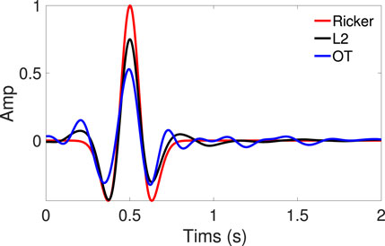
FIGURE 6. Final source wavelets with the event-based inversion strategy for L2 and J_t function.

FIGURE 7

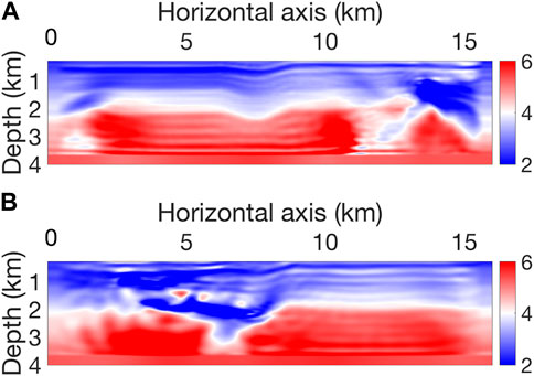
FIGURE 7. Final v_p model obtained with (A) L2 function and (B) J_t function.

3.4 Proposed combinatory strategy

We observed that an event-based inversion strategy helps recover the structure, but it is not sufficient with L2 or the OT objective function. We propose to apply the normalized cross-correlation function J_c first and then conduct an OT inversion. We still consider the event-based inversion strategy. In the J_c inversion, we select a long offset trace as the source wavelet and keep it fixed during the inversion. When the OT inversion is conducted, both the source wavelets and the model parameters are simultaneously updated.

The normalized cross-correlation function J_c is less sensitive to source wavelets, as shown in Figure 1. We choose a long offset seismic trace at X=15 km (blue line in Figure 5). We calculate the envelope of the whole trace and cut the seismic trace defined by the first envelope wavelet (we select the seismic trace, not the envelope). Figure 8 shows how we select the seismic wavelet. Its Fourier transform shows that the selected seismic wavelet has a different frequency content compared to the true source wavelet. Figure 9 shows the synthetic data corresponding to the cut seismic trace in the linearly increasing initial model. The initial seismograms are quite simple.

FIGURE 8

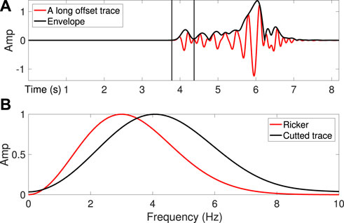
FIGURE 8. A long offset trace (marked with a blue line in Figure 5) is selected to build the initial source wavelet. The wavelet is not accurate in the (A) time or (B) frequency domain.

FIGURE 9

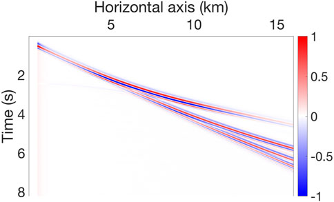
FIGURE 9. Initial synthetic in the linearly increasing initial model (Figure 4) with the cut trace (Figure 8) as the source wavelet.

The cross-correlation could map multiple events as sidelobes. This affects the adjoint source and the consequent gradient, leading to artifacts in the model. It is important to not include too many events under J_c. Otherwise, it is difficult to obtain an acceptable inversion. Figure 10 shows an inversion under J_c without using any time window. The initial source wavelet is the cut trace shown in Figure 8. The gradient does not show a correct direction update between the first and third dashed lines. The final model is not close to the true model.

FIGURE 10

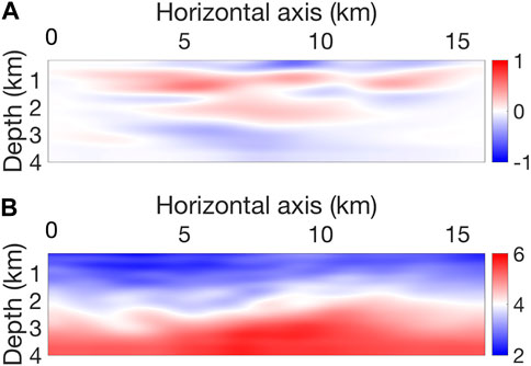
FIGURE 10. Inversion experiment under J_c function with the event-based inversion strategy. Entire seismograms are included at once. (A) Initial gradient. The cross-talk between events brings a lot of artifacts to the gradient. (B) Final v_p after 25 iterations.

The inversion using J_c is much better when the Gaussian time windows are used than the one without windows. For the total recording length T = 8.192 s, four inversion stages are conducted with the ratios $\frac{\sigma }{T}=0.02,0.05,0.1,0.2$. The first Gaussian time window keeps only the early arrival events. The gradient is shown in Figure 11. In comparison, we show the gradient of WET where a true source wavelet is used. The similarity indicates that J_c combined with Gaussian time windows can produce correct gradients even with a wrong source wavelet. The wider windows allow us to include more complex events. We stop at the ratio of 0.2. Later stages with bigger ratios introduce too much cross-talk between events to the adjoint source, and the model updating becomes negligible. A shot gather from the final synthetic data shown in Figure 12 shows that the global pattern of the observed data is captured. The final velocity model v_p is shown in Figure 13. The long-wavelength structures are retrieved. The fine-scale structures are not very satisfactory because of the cross-talk between seismic events when the Gaussian window becomes wide.

FIGURE 11

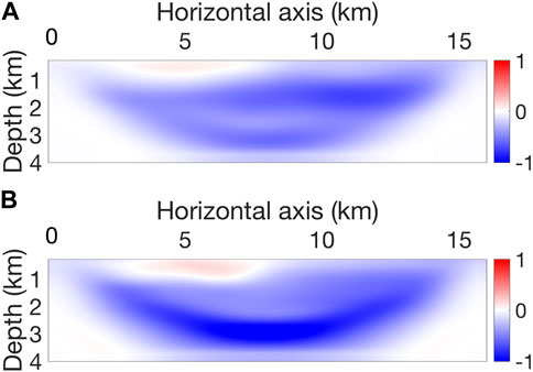
FIGURE 11. (A) Initial gradient under J_c with a Gaussian time window σ =0.02T. (B) Initial gradient of WET as a reference, where the true source wavelet is used.

FIGURE 12

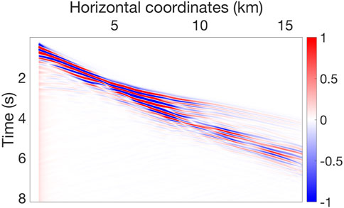
FIGURE 12. Final synthetics of the J_c inversion. The overall pattern of the observed data in Figure 5 is captured.

FIGURE 13

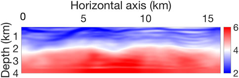
FIGURE 13. Final inverted v_p model of J_c inversion.

We continue the inversion by following an OT objective function. The Gaussian time windows are defined with ratios $\frac{\sigma }{T}=0.2,0.3,0.5$ in three stages. Figure 14 shows the estimated source wavelets for these three stages. The first wavelet clearly deviates from the true source wavelet. However, later source wavelets become closer and closer to the true source wavelet. The final v_p and ρ are shown in Figure 15. The continuous thin-layered structures along the first dashed line are well-retrieved in the v_p model. The inverted v_p model is much cleaner than the starting model and shows high-resolution, high-fidelity structures. The inverted ρ is overestimated in the deeper area below the second dashed line. Above the second dashed line, thin-layered structures are obtained. A shot gather from the final synthetic data is shown in Figure 16A. The final residuals shown in Figure 16B indicate that the early arrivals are not perfectly matched. The trace-by-trace comparison shown in Figure 17 indicates that the phases are fitted, but the amplitudes are not perfectly matched. The reason is that the Gardner law overestimated the density in the deep area; therefore, the inversion does not perfectly fit the amplitudes of the early arrivals.

FIGURE 14

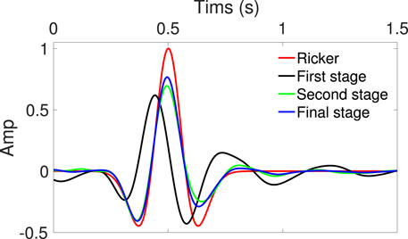
FIGURE 14. Estimated source wavelets of the J_t inversion, following the J_c inversion. The wavelets become closer and closer to the true source wavelet (Ricker wavelet).

FIGURE 15

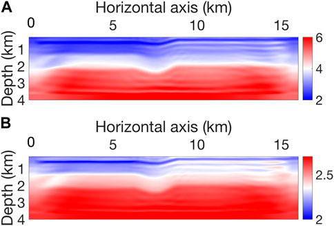
FIGURE 15. Final recovered model with our proposed inversion strategy. (A) Final v_p. (B) Final ρ. The model is well-recovered.

FIGURE 16

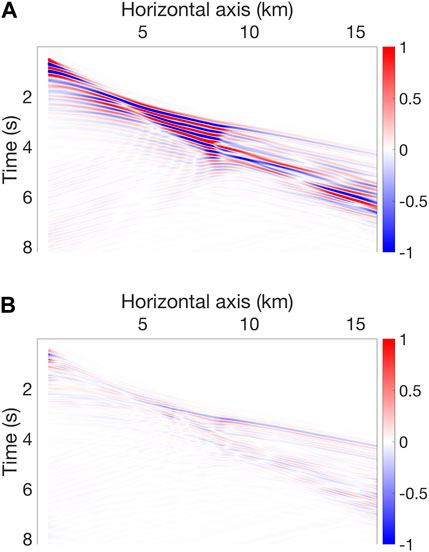
FIGURE 16. (A) Final synthetics in the inverted model shown in Figure 15. (B) Difference with the observed data. The inter-bed reflections and the scattered events are fitted. The worst fitness occurs at the long-offset early arrivals. A more detailed comparison, seismic trace comparison, is shown in Figure 17.

FIGURE 17

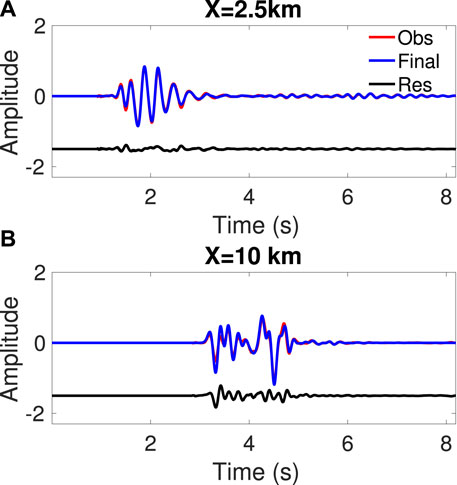
FIGURE 17. The final synthetics (blue) are compared to the observed trace (red) at short and long offsets. The phases are fitted better than the amplitudes. The residuals (black) are shifted downward when plotting.

4 Applications to the SEAM model and land seismic data

After building our inversion workflow, we carried out two experiments to verify the effectiveness and feasibility of the process. The first experiment is for the SEAM velocity model, which is a standard model often used to test inversion algorithms, and the second experiment is for land seismic data recorded in Southwest China, which are difficult to invert by a conventional FWI process.

4.1 SEAM model inversion

We observed, in the Middle East model, the presence of abundant diving waves in the data. To show the generalization of our proposed inversion flow, we now use the SEAM model, which is shown in Figure 18. Geologic layers are generally not horizontal for the SEAM model but are folding. There is also displacement of geologic layers. The velocity v_p increases slowly from top to bottom, unlike in the Middle East model. The initial velocity model v_p is also a 1D linearly increasing model, and the density is calculated from v_p via the same empirical relationship as that used in the Middle East model inversion. Figure 19 shows the initial v_p and ρ. We also overlap the traced rays for one shot in the initial model. The deepest ray penetrates only to approximately 1 km. The difference between the SEAM model and the Middle East model can also be observed in the seismograms. The observed data shown in Figure 21A are dominated by reflections.

FIGURE 18

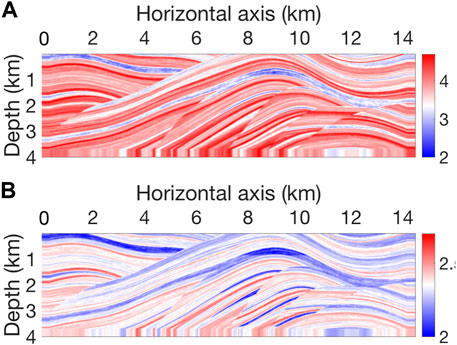
FIGURE 18. (A) True v_p and (B) true ρ. Geologic structures are twisted.

FIGURE 19

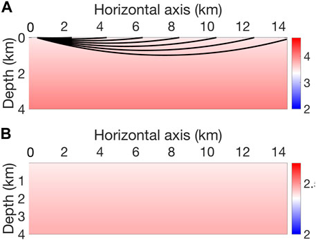
FIGURE 19. (A) Linearly increasing initial v_p and (B) deduced ρ via an empirical relationship. The deepest ray trace penetrates to approximately 1 km.

The inversion setting is the same as in the Middle East model inversion. We use the same source wavelet, consider a fixed seismic acquisition, and also consider the same inversion strategy. As we did in the Middle East model inversion, we select a long offset seismic trace and cut the first wavelet as the initial source wavelet. The final model after J_c inversion is shown in Figures 20A, B, which shows that the model is largely updated. Then, we continue the inversion with the OT objective function J_t. The final model is shown in Figures 20C, D. The twisted geologic structures are well-recovered from top to bottom. The final synthetic is shown in Figure 21B, which captures the pattern of the observed data shown in Figure 21A. The residual shown in Figure 21C also confirms that most of the events are matched. In the true model, the structures in the leftmost part would reflect seismic waves outside of the acquisition. This explains that the model is not well-recovered in the leftmost part. This is also consistent with the fact that the non-zero part of the residual is mainly short offset reflections.

FIGURE 20

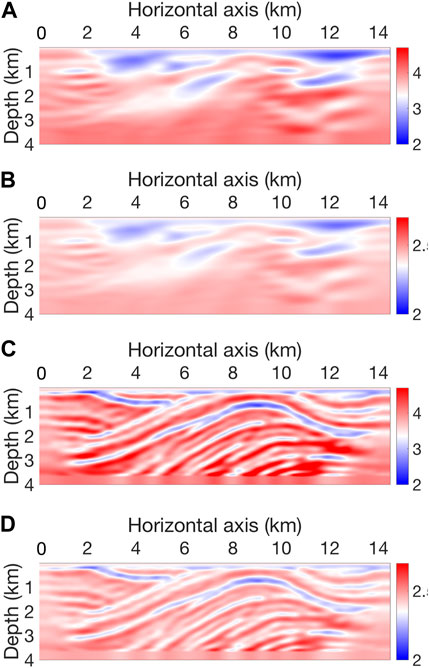
FIGURE 20. Final model of (A) v_p and (B) ρ after J_c inversion. A following J_t inversion correctly recovers (C) v_p and (D) ρ.

FIGURE 21

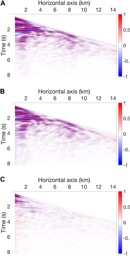
FIGURE 21. (A) Observed data. (B) Final synthetics. (C) Final residuals.

4.2 Land seismic data application in Sichuan Basin, Southwest China

We apply our inversion workflow to a real-land seismic dataset recorded in Southwest China. The land seismic data have been preprocessed to remove the surface waves and to correct for varying topography. The seismic survey is along a straight line. It is 75-km long. The shot spacing is not regular: it varies from 20 m to 200 m. Totally, we have 619 shots. For each shot, the offset is from approximately −6 to 6 km, with an inter-receiver spacing of 20 m. Thus, each shot is recorded by less than 600 geophones. The recording time is 2 s, and the time interval is 1 m. The processed observed data are shown in Figure 22A, which contains direct waves and reflections. The maximum frequency is approximately 15 Hz, while the lowest frequency is approximately 5 Hz. The initial model, shown in Figure 23A, is provided by an industrial routine process including ray tracing tomography. The initial synthetics are shown in Figure 22B. The interleave comparison shown in Figure 22C shows the data fitting of initial synthetics to the observed data.

FIGURE 22

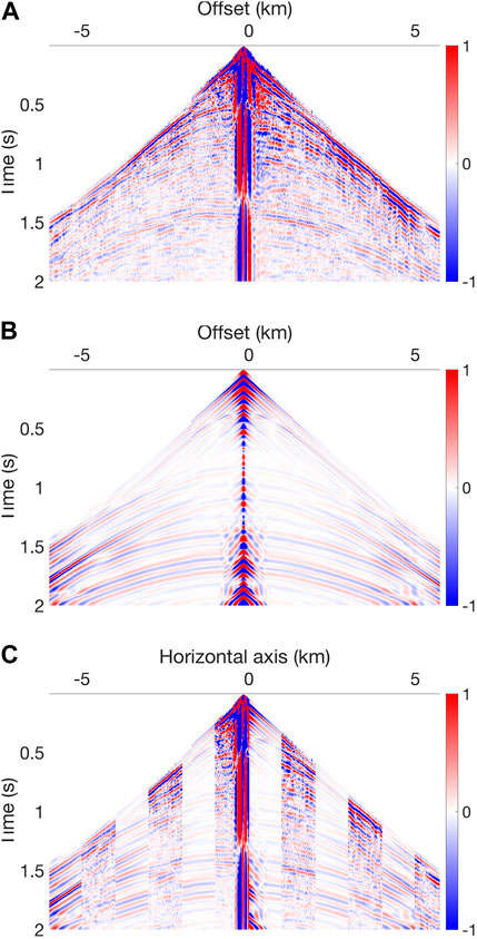
FIGURE 22. (A) Observed data, (B) initial synthetics, and (C) initial inter-leave data comparison.

FIGURE 23

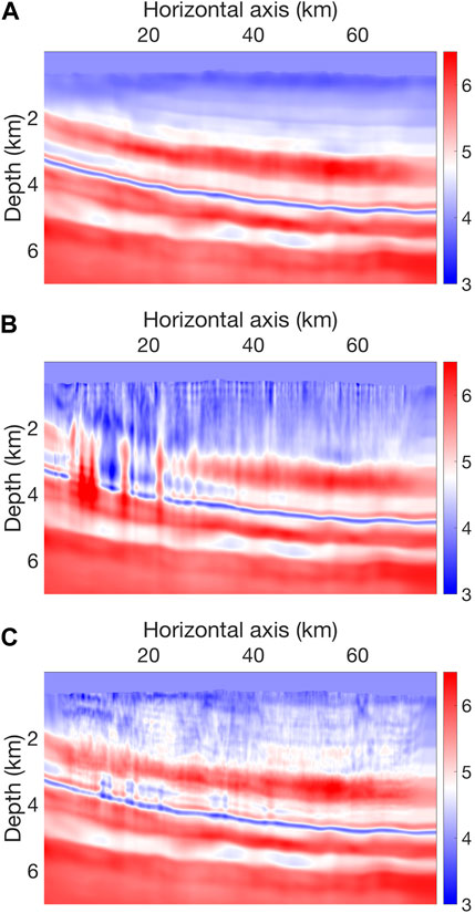
FIGURE 23. (A) Initial model, (B) inverted model by conventional least-squares function, and (C) inverted model by our inversion workflow.

Following our inversion workflow, we apply the normalized cross-correlation objective function in the first step. The model is updated a little bit. Then, in the second step, we parallel-run two inversions with the conventional least-squares objective function and OT objective function. In this second step, we divide the frequency band into three stages with the maximum frequency at 7 Hz, 9 Hz, and 15 Hz. In each frequency band, we run two inversions with a Gaussian window σ = 0.2T and without windows. The conventional inversion wildly updates the model, as shown in Figure 23B. The least-squares function is a point-by-point comparison process. Thus, the pattern of seismic events is not honored. When the adjoint source is back-propagated to assemble the gradient, artifacts emerge. At the end, model updating becomes inaccurate. Figure 23C shows the final model recovery with the OT objective function. Coherent structures are revealed. Fine structures are reconstructed. A well log comparison at X = 45.5 km is shown in Figure 24. The velocity down to 3 km is overestimated because we use a constant density inversion, so the effects of density are not taken into account in the final v_p model. High-frequency model variation is recovered. The final synthetics, shown in Figure 25A, are closer to the observed data than the initial synthetics. The inter-leave comparison shown in Figure 25B shows the data fitting of final synthetics to the observed data.

FIGURE 24

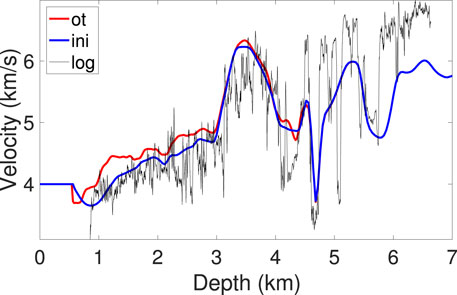
FIGURE 24. Comparison of final recovery to the well log.

FIGURE 25

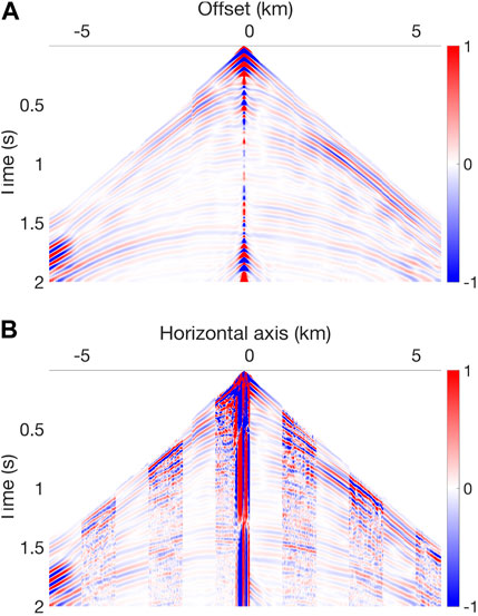
FIGURE 25. (A) Final synthetics. (B) Inter-leave comparison between the final synthetics and observed data.

5 Discussion

Cross-correlation has been used in FWI for a long time. Luo and Schuster (1991) extracted the travel time differences from the observed traces and the synthetic traces. A suitable window is usually necessary to assure that the two traces contain the same events, such as diving waves, refractions, or reflections. Isolating early arrivals is not too difficult, and the long-wavelength background could be reliably retrieved. However, adding later arrivals such as reflections to further increase the resolution of the inverted model is not an easy task. In addition, an incorrect source wavelet would strongly affect the travel time estimation. van Leeuwen and Mulder (2010) improved the objective function by exploiting the whole information on the cross-correlation instead of only the maximum value. Restriction on the design of the time windows is not as strict as WET. Another advantage is that the cross-correlation function is less sensitive to the source wavelet. The inaccuracy of the source wavelet is compensated by the adjoint source under the cross-correlation function. The disadvantage of the cross-correlation function is that the presence of multiple seismic events causes cross-talk, which is why we design a widening Gaussian window to gradually include more and more events in this study. Starting from fitting the early arrivals, later events are gradually incorporated. The cross-talk among events is thus carefully controlled. Regarding when we switch from J_c to other functions, we rely on the adjoint source (not the observed data). When the adjoint source contains many events, it is better to stop using J_c and switch to OT. The limitation to J_c in the presence of multiple events could also be inferred by the current FWI studies. There are not many academic literature studies or successful applications reported of using J_c. It is really because the multiple seismic events cannot be correctly handled by J_c.

Two kinds of penalty function are proposed by van Leeuwen and Mulder (2010): a linear function and a Gaussian function. However, we prefer to use the Gaussian function as the weighting function. In the presence of multiple events, the cross-correlation function contains cross-talks between different kinds of events, such as between diving waves and reflections. The Gaussian weighting function could mute signals at large lag-times. This raises the question of choosing the width of the Gaussian weighting function. In this study, we limit the maximum standard deviation to 0.2 of the length of the seismic trace, and it helps in recovering the Middle East and SEAM models.

In Ricker wavelet testing, we apply a 1D OT algorithm since only one pair of traces is present. We notice that 1D OT could produce triangular adjoint sources in the case of simple waveform comparison (for example, pure time shift events). This is not a problem for the inversion. In addition, we apply the 2D OT algorithm for FWI experiments. We process one shot gather instead of one trace at one time. A 2D OT objective function is much more convex than a 1D OT objective function (but 2D OT is computationally more expensive). It does not, however, mean that we can start from an arbitrary initial model. A reasonable model is still needed for an OT inversion. The assumption of OT is that the input should be positive, which is not true for oscillating seismic signals. In our OT algorithm, being positive is implicitly assumed when translating the OT problem to dual space. Thus, only the residual (δp_s,r) instead of individual traces matters. We do not need to shift the input seismic signals, but the assumption of being positive is not honored. This violation, in our opinion, really affects the convexity of the OT objective function. The benefit of the 2D OT objective function is that it is a global pattern-matching procedure. It is possible that the cross-correlation function could bring artifacts to the model. However, a following OT inversion can clean the model and produce fine structures.

In our proposed inversion workflow, we first apply the normalized cross-correlation function and continue the inversion with the optimal transport function. It remains unclear whether a L2 function instead of the optimal transport function is sufficient. We tested this. For the Middle East model inversion, a following L2 function could recover the model as good as the optimal transport function. That is because the seismograms are dominated by diving waves. In the SEAM model inversion, the seismograms are dominated by reflections. The inversion is more nonlinear than the Middle East model inversion. A following L2 function does not update the model retrieved by the normalized cross-correlation function. The OT objective function can also recover fine structures.

After carefully evaluating our inversion workflow, we apply it to the land seismic data in Southwest China with little modifications. We apply the cross-correlation function to update the model in the first step, followed by applying the OT objective function in the second step. The final model shows coherent lateral structures. Following the first step, we also apply the least-squares function, which showed inferior recovery.

6 Conclusion

We proposed to gradually include seismic events in the inversion process using Gaussian time windows and switch from a cross-correlation objective function to an OT objective function as the time window widens. In the first step with the cross-correlation function, we aim to mainly update the background. In the second step with an OT objective function, we aim to simultaneously update the source wavelets and the model parameters. For two different geological structures, the Middle East model and the SEAM model, we have recovered high-resolution and high-fidelity structures. At the end, we successfully applied our inversion strategy to a real-land seismic dataset recorded in Sichuan Basin, Southwest China, and obtained stable and high-resolution inversion results.

Data availability statement

The raw data supporting the conclusion of this article will be made available by the authors, without undue reservation.

Author contributions

JS: conceptualization, methodology, and writing–original draft and review and editing. ZY: funding acquisition, supervision, validation, and writing–review and editing. HC: supervision, conceptualization, funding acquisition, and writing–review and editing. WH: methodology and writing–review and editing. WP: methodology, validation, and writing–review and editing. ML: validation, writing–review and editing, and methodology. NT: validation, writing–review and editing, and visualization.

Funding

The author(s) declare financial support was received for the research, authorship, and/or publication of this article. This study was funded by the CNPC Science and Technology Major Project (grant no. 2023ZZ05, 2023ZZ05-05), the National Natural Science Foundation of China (grant nos 41504110 and 42004116), the 14th 5-Year Basic Research Program of CNPC (grant nos 2021DJ3502, 2021DJ3503, and 2021D3605), and the Science and Technology Fund Projects of PetroChina Company Limited (grant no. 2021DJ1803).

Conflict of interest

Authors JS, ZY, and ML were employed by China National Petroleum Corporation, and authors HC and NT were employed by Bureau of Geophysical Prospecting Inc.

The remaining author declares that the research was conducted in the absence of any commercial or financial relationships that could be construed as a potential conflict of interest.

Publisher’s note

All claims expressed in this article are solely those of the authors and do not necessarily represent those of their affiliated organizations, or those of the publisher, the editors, and the reviewers. Any product that may be evaluated in this article, or claim that may be made by its manufacturer, is not guaranteed or endorsed by the publisher.

References

Alkhalifah, T., and Choi, Y. (2014). From tomography to full-waveform inversion with a single objective function. Geophysics 79, R55–R61. doi:10.1190/geo2013-0291.1

CrossRef Full Text | Google Scholar

Alkhalifah, T. (2016). Full waveform inversion in an anisotropic world: where are the parameters hiding. EAGE publications.

Google Scholar

Bozdağ, E., Trampert, J., and Tromp, J. (2011). Misfit functions for full waveform inversion based on instantaneousphase and envelope measurements. Geophys. J. Int. 185, 845–870. doi:10.1111/j.1365-246x.2011.04970.x

CrossRef Full Text | Google Scholar

Brossier, R., Operto, S., and Virieux, J. (2009a). Robust frequency-domain full-waveform inversion using the l₁ norm. Geophys. Res. Lett. 36, L20310. doi:10.1029/2009GL039458

CrossRef Full Text | Google Scholar

Brossier, R., Operto, S., and Virieux, J. (2009b). Seismic imaging of complex onshore structures by 2D elastic frequency-domain full-waveform inversion. Geophysics 74, WCC105–WCC118. doi:10.1190/1.3215771

CrossRef Full Text | Google Scholar

Brossier, R., Operto, S., and Virieux, J. (2010). Which data residual norm for robust elastic frequency-domain full waveform inversion? Geophysics 75, R37–R46. doi:10.1190/1.3379323

CrossRef Full Text | Google Scholar

Bube, K. P., and Langan, R. T. (1997). Hybrid l₁/l₂ minimization with applications to tomography. Geophysics 62, 1183–1195. doi:10.1190/1.1444219

CrossRef Full Text | Google Scholar

Bunks, C., Salek, F. M., Zaleski, S., and Chavent, G. (1995). Multiscale seismic waveform inversion. Geophysics 60, 1457–1473. doi:10.1190/1.1443880

CrossRef Full Text | Google Scholar

Chi, B., Dong, L., and Liu, Y. (2014). Full waveform inversion method using envelope objective function without low frequency data. J. Appl. Geophys. 109, 36–46. doi:10.1016/j.jappgeo.2014.07.010

CrossRef Full Text | Google Scholar

Choi, Y., and Alkhalifah, T. (2011). Source-independent time-domain waveform inversion using convolved wavefields: application to the encoded multisource waveform inversion. Geophysics 76 (5), R125–R134. doi:10.1190/geo2010-0210.1

CrossRef Full Text | Google Scholar

Choi, Y., and Alkhalifah, T. (2017). Time-domain full waveform inversion of exponentially damped wavefield using the deconvolution-based objective function. Geophysics 83, R77–R88. doi:10.1190/geo2017-0057.1

CrossRef Full Text | Google Scholar

Claerbout, J. F., and Muir, F. (1973). Robust modeling with erratic data. Geophysics 38, 826–844. doi:10.1190/1.1440378

CrossRef Full Text | Google Scholar

Dahlen, F. A., Hung, S. H., and Nolet, G. (2000). Fréchet kernels for finite-frequency traveltimes-I. Theory. Geophys. J. Int. 141, 157–174. doi:10.1046/j.1365-246x.2000.00070.x

CrossRef Full Text | Google Scholar

Djebbi, R., and Alkhalifah, T. (2014). Traveltime sensitivity kernels for wave equation tomography using the unwrapped phase. Geophys. J. Int. 197, 975–986. doi:10.1093/gji/ggu025

CrossRef Full Text | Google Scholar

Dutta, G., Sinha, M., and Schuster, G. T. (2014). “A cross-correlation objective function for least-squares migration and visco-acoustic imaging,” in SEG technical program expanded abstracts 2014 (Society of Exploration Geophysicists), 3985–3990.

CrossRef Full Text | Google Scholar

Engquist, B., and Froese, B. D. (2014). Application of the Wasserstein metric to seismic signals. Commun. Math. Sci. 12, 979–988. doi:10.4310/cms.2014.v12.n5.a7

CrossRef Full Text | Google Scholar

Engquist, B., Froese, B. D., and Yang, Y. (2016). Optimal transport for seismic full waveform inversion. Commun. Math. Sci. 14, 2309–2330. doi:10.4310/cms.2016.v14.n8.a9

CrossRef Full Text | Google Scholar

Ferradans, S., Papadakis, N., Peyré, G., and Aujol, J.-F. (2014). Regularized discrete optimal transport. SIAM J. Imaging Sci. 7, 1853–1882. doi:10.1137/130929886

CrossRef Full Text | Google Scholar

Gardner, G. H. F., Gardner, L. W., and Gregory, A. R. (1974). Formation velocity and density–the diagnostic basics for stratigraphic traps. Geophysics 39, 770–780. doi:10.1190/1.1440465

CrossRef Full Text | Google Scholar

Gauthier, O., Virieux, J., and Tarantola, A. (1986). Two-dimensional nonlinear inversion of seismic waveforms: numerical results. Geophysics 51, 1387–1403. doi:10.1190/1.1442188

CrossRef Full Text | Google Scholar

Guitton, A., and Symes, W. W. (2003). Robust inversion of seismic data using the Huber norm. Geophysics 68, 1310–1319. doi:10.1190/1.1598124

CrossRef Full Text | Google Scholar

Ha, T., Chung, W., and Shin, C. (2009). Waveform inversion using a back-propagation algorithm and a Huber function norm. Geophysics 74, R15–R24. doi:10.1190/1.3112572

CrossRef Full Text | Google Scholar

Hamilton, E. L. (1978). Sound velocity–density relations in sea-floor sediments and rocks. J. Acoust. Soc. Am. 63, 366–377. doi:10.1121/1.381747

CrossRef Full Text | Google Scholar

He, W., Plessix, R.-É., and Singh, S. (2018). Parameterization study of the land multi-parameter VTI elastic waveform inversion. Geophys. J. Int. 213, 1662–1674. doi:10.1093/gji/ggy099

CrossRef Full Text | Google Scholar

Hörmann, G., and De Hoop, M. V. (2002). Detection of wave front set perturbations via correlation: foundation for wave-equation tomography. Appl. Anal. 81, 1443–1465. doi:10.1080/0003681021000035489

CrossRef Full Text | Google Scholar

Huang, Y. (2014). “A misfit function tolerating inconsistent data,” in SEG technical program expanded abstracts (Society of Exploration Geophysicists), 4660–4664.

CrossRef Full Text | Google Scholar

Huber, P. J. (1973). Robust regression: asymptotics, conjectures, and Monte Carlo. Ann. Statistics 1, 799–821. doi:10.1214/aos/1176342503

CrossRef Full Text | Google Scholar

Kennett, B. L., and Fichtner, A. (2012). A unified concept for comparison of seismograms using transfer functions. Geophys. J. Int. 191, 1403–1416. doi:10.1111/j.1365-246x.2012.05693.x

CrossRef Full Text | Google Scholar

Lailly, P. (1983). “The seismic inverse problem as a sequence of before stack migrations,” in Conference on inverse scattering, theory and application, society for industrial and applied mathematics. Editors R. Bednar, and A. Weglein (Philadelphia, 206–220.

Google Scholar

Lellmann, J., Lorenz, D., Schönlieb, C., and Valkonen, T. (2014). Imaging with kantorovich–rubinstein discrepancy. SIAM J. Imaging Sci. 7, 2833–2859. doi:10.1137/140975528

CrossRef Full Text | Google Scholar

Li, Z., Wang, Z., Huang, J., and Cui, C. (2022). Multi-scale full waveform inversion based ongradient decomposition in wavenumber domain. Chin. J. Geophys. (in Chinese) 65, 2693–2703. doi:10.6038/cjg2022P0508

CrossRef Full Text | Google Scholar

Liu, Q., and Tromp, J. (2006). Finite-frequency kernels based on adjoint methods. Bulletin of the Seismological Society of America 96, 2383–2397. doi:10.1785/0120060041

CrossRef Full Text | Google Scholar

Liu, Y., Teng, J., Xu, T., Wang, Y., Liu, Q., and Badal, J. (2017). Robust time-domain full waveform inversion with normalized zero-lag cross-correlation objective function. Geophysical Journal International 209, ggw485–122. doi:10.1093/gji/ggw485

CrossRef Full Text | Google Scholar

Luo, J., and Wu, R.-S. (2015). Seismic envelope inversion: reduction of local minima and noise resistance. Geophysical Prospecting 63, 597–614. doi:10.1111/1365-2478.12208

CrossRef Full Text | Google Scholar

Luo, S., and Sava, P. (2011). A deconvolution-based objective function for wave-equation inversion. SEG Technical Program Expanded Abstracts 30, 2788–2792. doi:10.1190/1.3627773

CrossRef Full Text | Google Scholar

Luo, Y., and Schuster, G. T. (1991). Wave-equation traveltime inversion. Geophysics 56, 645–653. doi:10.1190/1.1443081

CrossRef Full Text | Google Scholar

Maarten, V., and van Der Hilst, R. D. (2005). On sensitivity kernels for wave-equation transmission tomography. Geophysical Journal International 160, 621–633. doi:10.1111/j.1365-246x.2004.02509.x

CrossRef Full Text | Google Scholar

Métivier, L., Brossier, R., Mérigot, Q., Oudet, E., and Virieux, J. (2016b). An optimal transport approach for seismic tomography: application to 3D full waveform inversion. Inverse Problems 32, 115008. doi:10.1088/0266-5611/32/11/115008

CrossRef Full Text | Google Scholar

Métivier, L., Brossier, R., Mérigot, Q., Oudet, E., and Virieux, J. (2016a). Measuring the misfit between seismograms using an optimal transport distance: application to full waveform inversion. Geophysical Journal International 205, 345–377. doi:10.1093/gji/ggw014

CrossRef Full Text | Google Scholar

Nocedal, J. (1980). Updating quasi-Newton matrices with limited storage. Mathematics of Computation 35, 773–782. doi:10.1090/s0025-5718-1980-0572855-7

CrossRef Full Text | Google Scholar

Nolet, G. (2008). A breviary of seismic tomography. Cambridge, UK: Cambridge University Press.

Google Scholar

Plessix, R. E. (2006). A review of the adjoint-state method for computing the gradient of a functional with geophysical applications. Geophysical Journal International 167, 495–503. doi:10.1111/j.1365-246x.2006.02978.x

CrossRef Full Text | Google Scholar

Plessix, R. E., and Cao, Q. (2011). A parametrization study for surface seismic full waveform inversion in an acoustic vertical transversely isotropic medium. Geophysical Journal International 185, 539–556. doi:10.1111/j.1365-246X.2011.04957.x

CrossRef Full Text | Google Scholar

Poncet, R., Messud, J., Bader, M., Lambaré, G., Viguier, G., and Hidalgo, C. (2018). “Fwi with optimal transport: a 3D implementation and an application on a field dataset,” in Expanded abstracts, 80^th annual EAGE meeting (copenhagen).

CrossRef Full Text | Google Scholar

Pratt, R. G. (1999). Seismic waveform inversion in the frequency domain, Part 1: theory and verification in a physical scale model. Geophysics 64, 888–901. doi:10.1190/1.1444597

CrossRef Full Text | Google Scholar

Pratt, R. G. (2004). “Velocity models from frequency-domain waveform tomography: past, present and future,” in Expanded abstracts (eur. Ass. Expl. Geophys.).

CrossRef Full Text | Google Scholar

Routh, P., Krebs, J., Lazaratos, S., Baumstein, A., Chikichev, I., Lee, S., et al. (2011a). “Full-wavefield inversion of marine streamer data with the encoded simultaneous source method,” in Expanded abstracts, 73^thAnnual meeting (EAGE).

Google Scholar

Routh, P., Krebs, J., Lazaratos, S., Baumstein, A., Lee, S., Cha, Y. H., et al. (2011b). “Encoded simultaneous source full-wavefield inversion for spectrally shaped marine streamer data,” in SEG technical program expanded abstracts 2011 30, 2433–2438. doi:10.1190/1.3627697

CrossRef Full Text | Google Scholar

Shin, C., and Ha, W. (2008). A comparison between the behavior of objective functions for waveform inversion in the frequency and laplace domains. Geophysics 73, VE119–VE133. doi:10.1190/1.2953978

CrossRef Full Text | Google Scholar

Shipp, R. M., and Singh, S. C. (2002). Two-dimensional full wavefield inversion of wide-aperture marine seismic streamer data. Geophysical Journal International 151, 325–344. doi:10.1046/j.1365-246x.2002.01645.x

CrossRef Full Text | Google Scholar

Song, J., Cao, H., Yang, Z., and Hu, X. (2019). “Application of full waveform inversion to land seismic data in Sichuan Basin, Southwest China,” in SEG technical program expanded abstracts 2019. doi:10.1190/segam2019-3216517.1

CrossRef Full Text | Google Scholar

Song, J., Shi, Y., Xu, J., Li, J., Li, Y., and Cui, X. (2015). “Elastic Full Waveform Inversion with envelope based misfit function,” in SEG technical program expanded abstracts 2015, 1479–1484. doi:10.1190/segam2015-5921592.1

CrossRef Full Text | Google Scholar

Sun, B., and Alkhalifah, T. (2019a). Adaptive traveltime inversion. Geophysics 84, U13–U29. doi:10.1190/geo2018-0595.1

CrossRef Full Text | Google Scholar

Sun, B., and Alkhalifah, T. (2019b). The application of an optimal transport to a preconditioned data matching function for robust waveform inversion. Geophysics 84, R923–R945. doi:10.1190/geo2018-0413.1

CrossRef Full Text | Google Scholar

Tao, K., Grand, S. P., and Niu, F. (2017). Full-waveform inversion of triplicated data using a normalized-correlation-coefficient-based misfit function. Geophysical Journal International 210, 1517–1524. doi:10.1093/gji/ggx249

CrossRef Full Text | Google Scholar

Tarantola, A. (1984). Inversion of seismic reflection data in the acoustic approximation. Geophysics 49, 1259–1266. doi:10.1190/1.1441754

CrossRef Full Text | Google Scholar

Tarantola, A. (1987). “Inversion of travel times and seismic waveforms,” in Seismic tomography (Springer), 135–157.

CrossRef Full Text | Google Scholar

van Leeuwen, T., and Mulder, W. A. (2010). A correlation-based misfit criterion for wave-equation traveltime tomography. Geophysical Journal International 182, 1383–1394. doi:10.1111/j.1365-246x.2010.04681.x

CrossRef Full Text | Google Scholar

van Leeuwen, T., and Mulder, W. (2008). Velocity analysis based on data correlation. Geophysical Prospecting 56, 791–803. doi:10.1111/j.1365-2478.2008.00704.x

CrossRef Full Text | Google Scholar

Virieux, J., and Operto, S. (2009). An overview of full waveform inversion in exploration geophysics. Geophysics 74, WCC1–WCC26. doi:10.1190/1.3238367

CrossRef Full Text | Google Scholar

Virieux, J. (1986). P-SV wave propagation in heterogeneous media: velocity-stress finite difference method. Geophysics 51, 889–901. doi:10.1190/1.1442147

CrossRef Full Text | Google Scholar

Wang, H., Singh, S., Audebert, F., and Calandra, H. (2015). Inversion of seismic refraction and reflection data for building long-wavelength velocity models. Geophysics 80, R81–R93. doi:10.1190/geo2014-0174.1

CrossRef Full Text | Google Scholar

Wang, H., Singh, S., and Calandra, H. (2014). Integrated inversion using combined wave-equation tomography and full-waveform inversion. Geophysical Journal International 198, 430–446. doi:10.1093/gji/ggu138

CrossRef Full Text | Google Scholar

Wang, Y., and Rao, Y. (2009). Reflection seismic waveform tomography. Journal of Geophysical Research 114, 1978–2012. doi:10.1029/2008jb005916

CrossRef Full Text | Google Scholar

Warner, M., and Guasch, L. (2014). “Adaptative waveform inversion - FWI without cycle skipping - theory,” in 76th EAGE conference and exhibition 2014. We E106 13. doi:10.3997/2214-4609.20141092

CrossRef Full Text | Google Scholar

Woodward, M. J. (1992). Wave-equation tomography. Geophysics 57, 15–26. doi:10.1190/1.1443179

CrossRef Full Text | Google Scholar

Wu, R.-S., Luo, J., and Wu, B. (2014). Seismic envelope inversion and modulation signal model. Geophysics 79, WA13–WA24. doi:10.1190/geo2013-0294.1

CrossRef Full Text | Google Scholar

Yang, Y., Engquist, B., Sun, J., and Hamfeldt, B. F. (2018). Application of optimal transport and the quadratic Wasserstein metric to full-waveform inversion. Geophysics 83, R43–R62. doi:10.1190/geo2016-0663.1

CrossRef Full Text | Google Scholar

YongHuangLi, P. J. Z., Liao, W., and Qu, L. (2019b). Least-squares reverse time migration via linearized waveform inversion using a Wasserstein metric. Geophysics 84, S411–S423. doi:10.1190/geo2018-0619.1

CrossRef Full Text | Google Scholar

YongLiaoHuang, P. W. J., Li, Z., and Lin, Y. (2019a). Misfit function for full waveform inversion based on the Wasserstein metric with dynamic formulation. Journal of Computational Physics 399, 108911. doi:10.1016/j.jcp.2019.108911

CrossRef Full Text | Google Scholar

Yuan, Y. O., and Simons, F. J. (2014). Multiscale adjoint waveform-difference tomography using wavelets. Geophysics 79, WA79–WA95. doi:10.1190/geo2013-0383.1

CrossRef Full Text | Google Scholar

Zhang, Q., Zhou, H., Li, Q., Chen, H., and Wang, J. (2016). Robust source-independent elastic full-waveform inversion in the time domain. Geophysics 81, R29–R44. doi:10.1190/geo2015-0073.1

CrossRef Full Text | Google Scholar

Zhang, Y., and Wang, D. (2009). Traveltime information-based wave-equation inversion. Geophysics 74, WCC27–WCC36. doi:10.1190/1.3243073

CrossRef Full Text | Google Scholar

Zhang, Z., Alkhalifah, T., Wu, Z., Liu, Y., He, B., and Oh, J. (2019). Normalized nonzero-lag crosscorrelation elastic full waveform inversion. Geophysics 84, 1JF–R10. doi:10.1190/geo2018-0082.1

CrossRef Full Text | Google Scholar