Source-independent elastic envelope inversion using the convolution method

Elastic full waveform inversion (EFWI) is a powerful technique. However, its strong non-linearity makes it susceptible to converging towards local extremes during the iterative process due to various factors like insufficient low-frequency information or an inadequate initial model. The existing elastic envelope inversion can offer a promising initial model for EFWI when low-frequency information is unavailable, reducing the dependence on both the initial model and low-frequency data. However, its accuracy is affected by the quality of the source wavelet, potentially causing the EFWI to run in the wrong direction if there is a discrepancy between the simulated wavelet and the field wavelet. To address these issues and enhance the reconstruction of large-scale information in the model, we propose a novel approach called source-independent elastic envelope inversion, employing the convolution method. By combining this method with source-independent multiscale EFWI, we effectively establish P- and S-wave velocity models even in situations with inaccurate wavelet information. The results of testing on a portion of the Marmousi2 model demonstrate the effectiveness of this technique for both full-band and low-frequency missing data scenarios.

1 Introduction

In multicomponent seismic exploration, establishing depth domain interval velocity models for compressional waves (P-wave) and shear waves (S-wave) is a key step in data imaging processing and inversion. Compared to techniques such as tomography and migration velocity analysis that only use travel time to obtain velocity information, elastic wave full waveform inversion (EFWI) utilizes information such as travel time, phase, and amplitude of elastic waves to establish P- and S-wave velocity models by minimizing the residual between the observed multicomponent data and simulated multicomponent seismic data of a specific velocity model. Therefore, EFWI has the potential to reveal structural details and lithology in complex geological backgrounds, and theoretically can obtain high-resolution depth domain P- and S-wave velocity models.

The idea of full waveform inversion (FWI) of seismic waves was first proposed by Lailly (1983) and Tarantola (1984). Under the theoretical framework of generalized least squares, FWI calculates the gradient by correlating the simulated wave field and the reverse wave field of the residual record between simulated and observed seismic data, and then updates the parameter model through continuous iteration. Since FWI can make full use of the kinematic and dynamic information of seismic waves to estimate the propagation speed of seismic waves and theoretically can obtain a higher resolution velocity model, the idea of FWI has received extensive research interest since it was proposed and research progress has been made in the objective function optimization (Datta et al., 2016; Zhu et al., 2016), multi-scale inversion (Bunks et al., 1995; Boonyasiriwat et al., 2009; Xu et al., 2014), mixed domain inversion (Kim et al., 2013; Jun et al., 2014; Xu et al., 2014), envelope inversion (Wu et al., 2013; Wu et al., 2014; Ao et al., 2015), source wavelet inversion (Tarantola, 1984; Song et al., 1995; Hu et al., 2017), and inversion efficiency improvement (Krebs et al., 2009; Wang et al., 2011) of FWI. Currently, FWI has been widely used in field seismic data imaging and many application examples have significantly improved the imaging quality of seismic data (Sirgue et al., 2010; Lewis et al., 2014; Liu et al., 2014; Zhong et al., 2017).

Tarantola (1986) and Pratt (1990) extended the compressional wave FWI to EFWI. Although some ideas and techniques in longitudinal wave FWI can be extended or even directly applied in EFWI, the non-linearity of inversion is further exacerbated by the inclusion of more inversion parameters in EFWI, and due to the presence of various types of noise in seismic data, EFWI based on three-component waveform matching is very sensitive to these noises, and the inversion is easily affected by these noises and falls into local extrema. At the same time, if the minimum available frequency in the three-component seismic data is too high, it will greatly enhance the dependence of EFWI on the initial model, and it is difficult to obtain good inversion results when the accuracy of the initial model is low. In addition, when the source wavelet is inaccurate, there is a significant difference between the synthetic data obtained from the erroneous source wavelet and observed data, which often leads to the wrong direction of EFWI and increases the difficulty of its application.

The lack of low-frequency information in observed three-component seismic data is one of the key factors leading to a decrease in the accuracy of EFWI. Baeten et al. (2013) pointed out that the low-frequency information of 1.5∼2 Hz in seismic records is particularly important for alleviating the “cycle skipping” phenomenon in FWI. The key to solving this problem is how to provide an accurate initial model for FWI when low-frequency information is missing. Envelope inversion is often used to construct the initial model of FWI. Bozdağ et al. (2011) pointed out that the seismic envelope contains rich low-frequency information and using the envelope as input data for FWI inversion can establish a more accurate initial model. The research of Huang et al. (2015) indicates that envelope inversion can significantly improve the accuracy of the inversion of the compressional and shear wave velocity model when seismic data lack low-frequency information. Wu and Chen (2017, 2018, 2020) proposed the direct envelope Fréchet derivative and the direct envelope inversion (DEI) method, which can map the ultra-low frequency envelope data perturbation to the velocity perturbation directly and can invert the large scale strong-scattering velocity model without low-frequency information in original common shot gathers. Chen et al. (2018) combined the DEI method with the wavefield direction decomposition method and proposed a reflection DEI method, which can improve the inversion effects of the velocity structures in the strong-scattering shielding area. However, traditional envelope inversion is based on the accurate source wavelet assumption. When the source wavelet is inaccurate, envelope inversion cannot construct a reasonable initial model. Therefore, Ao et al. (2015) proposed a convolutional envelope objective function based on the compressional equation, which can eliminate the impact of wavelet inaccuracy on the accuracy of compressional envelope inversion.

We extend the source-independent FWI (Choi et al., 2005) to EFWI to improve the accuracy of envelope inversion when the source wavelet is inaccurate. On the basis of previous research, a misfit function for the elastic wave convolution envelope was established, and corresponding gradient and adjoint source formulas were derived. Applying these methods to mixed domain EFWI can improve the inversion accuracy of compressional and shear wave velocity models in cases of wavelet inaccuracy and missing low-frequency information.

2 Source independent EFWI based on convolved elastic wavefields

The misfit function of EFWI in the time domain can be written as (Tarantola, 1986; Prat, 1990):

$E\left(\mathbf{m}\right)=\frac{1}{2}{\displaystyle \sum _{i=1}^{Ns}}{\displaystyle \sum _{j=1}^{Nr}}{\int }_0^T\left[{\left({\mathbf{u}}_{i,j}-{\mathbf{d}}_{i,j}\right)}^2\right]dt,(1)$

where $\mathbf{m}=\left(v_p,v_s\right)$, $v_p$ is the compression wave velocity, $v_s$ is the shear wave velocity, $Ns$ and $Nr$ are the shot number and receiver number per shot, respectively, and $\mathbf{u}$ and $\mathbf{d}$ are the modeled and observed three-component vector wave fields, respectively.

For each shot gather, select ${\mathbf{u}}_{i,k}$ and ${\mathbf{d}}_{i,k}$ as the reference traces of the modeled and the observed data, respectively, and $k$ as the channel number of the reference trace. Convolve the simulated traces with the reference traces of observed wavefields to obtain the modeled wavefields, and convolve the observed traces with the reference traces of simulated wavefields to obtain the modeled wavefields. So Eq. 1 becomes a new convolution misfit function:

$E_{cv}\left(\mathbf{m}\right)=\frac{1}{2}{\displaystyle \sum _{i=1}^{Ns}}{\displaystyle \sum _{j=1}^{Nr}}{\int }_0^T\left[{\left({\mathbf{u}}_{i,j}*{\mathbf{d}}_{i,k}-{\mathbf{d}}_{i,j}*{\mathbf{u}}_{i,k}\right)}^2\right]dt,(2)$

since the seismic traces of any components in the three-component seismic data can be regarded as Green’s function and source wavelet convolution, that is:

$d\left(t\right)=g\left(t\right)*s\left(t\right),(3)$

where $d$ is a certain component in the three-component data, $g$ is the Green’s function, and $s$ is the source wavelet.

Equation 2 can be expressed as:

$E_{cv}\left(\mathbf{m}\right)=\frac{1}{2}{\displaystyle \sum _{i=1}^{Ns}}{\displaystyle \sum _{j=1}^{Nr}}{\int }_0^{\mathrm{T}}\left[{\left({\mathbf{g}}_{i,j}^{\mathbf{u}}*{\mathbf{g}}_{i,k}^{\mathbf{d}}*{\mathbf{s}}_i^{\mathbf{d}}*{\mathbf{s}}_i^{\mathbf{u}}-{\mathbf{g}}_{i,j}^{\mathbf{d}}*{\mathbf{g}}_{i,k}^{\mathbf{u}}*{\mathbf{s}}_i^{\mathbf{d}}*{\mathbf{s}}_i^{\mathbf{u}}\right)}^2\right]dt,(4)$

where ${\mathbf{g}}^{\mathbf{u}}$ is the Green’s function of modeled three-component data, ${\mathbf{g}}^{\mathbf{d}}$ is the Green’s function of observed three-component data, and ${\mathbf{s}}^{\mathbf{u}}$ and ${\mathbf{s}}^{\mathbf{d}}$ are the source wavelet of modeled and observed three-component data, respectively.

From Eq. 4, we can see that for a shot gather, two terms in the time integration contain the same form of source ${\mathbf{s}}_i^{\mathbf{d}}*{\mathbf{s}}_i^{\mathbf{u}}$; therefore, we can use the convolution misfit function in EFWI to eliminate the influence of the source wavelet. This is the basic principle of the time domain convolution method to eliminate the influence of wavelets.

For frequency domain EFWI, since the time domain convolution operation is equivalent to the frequency domain multiplication operation, the source free misfit function of EFWI in the frequency domain in the two-dimensional case can be expressed as:

$E_{cv1}\left(\mathbf{m}\right)=\frac{1}{2}\mathfrak{R}{\displaystyle \sum _{i=1}^{Ns}}{\displaystyle \sum _{j=1}^{Nr}}{\left[\begin{array}{c}{U}_{i,k}^x{D}_{i,j}^x-D_{i,k}^x{U}_{i,j}^x\\ U_{i,k}^z{D}_{i,j}^z-D_{i,k}^z{U}_{i,j}^z\end{array}\right]}^{\mathrm{T}}\left[\begin{array}{c}{\left(U_{i,k}^x{D}_{i,j}^x-D_{i,k}^x{U}_{i,j}^x\right)}^{*}\\ {\left(U_{i,k}^z{D}_{i,j}^z-D_{i,k}^z{U}_{i,j}^z\right)}^{*}\end{array}\right],(5)$

where $U_{i,j}^x$, $U_{i,j}^z$, $D_{i,j}^x$, and $D_{i,j}^z$ are the X and Z components of the modeled wavefields and observed wavefields in the frequency domain, respectively, $U_{i,k}^x$, $U_{i,k}^z$, $D_{i,k}^x$, and $D_{i,k}^z$ are the X and Z components of reference traces of modeled wavefields and observed wavefields in the frequency domain, respectively, the superscript $\mathrm{T}$ is the transpose operator, the superscript $*$ is the conjugate operator, and $\mathfrak{R}$ is the real part operator.

The seismic wave in the frequency domain can also be regarded as the product of Green’s function and the source wavelet, so there are:

$D\left(\omega \right)=G\left(\omega \right)S\left(\omega \right),(6)$

where $D$ is the frequency domain seismic wave, $G$ is the frequency domain Green’s function, $S$ is the source wavelet in the frequency domain, and $\omega$ is the angular frequency.

According to Eq. 6, Eq. 5 can be expressed as:

$E_{cv1}\left(\mathbf{m}\right)=\frac{1}{2}\mathfrak{R}{\displaystyle \sum _{i=1}^{Ns}}{\displaystyle \sum _{j=1}^{Nr}}{\left[\begin{array}{c}{G}_{i,j}^{U^x}{G}_{i,k}^{D^x}{S}_i^{D^x}{S}_i^{U^x}-G_{i,j}^{D^x}{G}_{i,k}^{U^x}{S}_i^{D^x}{S}_i^{U^x}\\ G_{i,j}^{U^z}{G}_{i,k}^{D^z}{S}_i^{D^z}{S}_i^{U^z}-G_{i,j}^{D^z}{G}_{i,k}^{U^z}{S}_i^{D^z}{S}_i^{U^z}\end{array}\right]}^{\mathrm{T}}\left[\begin{array}{c}{\left(G_{i,j}^{U^x}{G}_{i,k}^{D^x}{S}_i^{D^x}{S}_i^{U^x}-G_{i,j}^{D^x}{G}_{i,k}^{U^x}{S}_i^{D^x}{S}_i^{U^x}\right)}^{*}\\ {\left(G_{i,j}^{U^z}{G}_{i,k}^{D^z}{S}_i^{D^z}{S}_i^{U^z}-G_{i,j}^{D^z}{G}_{i,k}^{U^z}{S}_i^{D^z}{S}_i^{U^z}\right)}^{*}\end{array}\right],(7)$

where $G_{i,j}^{U^x}$ and $G_{i,j}^{U^z}$ are the Green’s functions of modeled X and Z components in the frequency domain, respectively, $G_{i,j}^{D^x}$ and $G_{i,j}^{D^z}$ are the Green’s functions of observed X and Z components in the frequency domain, respectively, $S_{i,j}^{U^x}$ and $S_{i,j}^{U^z}$ are the source wavelets of modeled X and Z components in the frequency domain, respectively, and $S_{i,j}^{D^x}$ and $S_{i,j}^{D^z}$ are the source wavelets of observed X and Z components in the frequency domain, respectively.

From Eq. 7, it can be seen that both sides of each minus have the same form of source terms. By using this misfit function, the influence of wavelet differences between simulated and observed records is eliminated, which is the basic principle of eliminating the influence of wavelets in frequency domain EFWI.

Make $R_{i,j}^x=U_{i,k}^x{D}_{i,j}^x-D_{i,k}^x{U}_{i,j}^x$ and $R_{i,j}^z=U_{i,k}^z{D}_{i,j}^z-D_{i,k}^z{U}_{i,j}^z$, Eq. 7 can be expressed as:

$E_{cv1}\left(\mathbf{m}\right)=\frac{1}{2}\mathfrak{R}{\displaystyle \sum _{i=1}^{Ns}}{\displaystyle \sum _{j=1}^{Nr}}{\left[\begin{array}{c}{R}_{i,j}^x\\ R_{i,j}^z\end{array}\right]}^{\mathrm{T}}\bullet \left[\begin{array}{c}{R_{i,j}^x}^{*}\\ {R_{i,j}^z}^{*}\end{array}\right].(8)$

By taking the partial derivative of $\mathbf{m}$ on both sides of the above equation and using the elastic wave equation to obtain $R_{i,j}^x$ and $R_{i,j}^z$, the gradient formula in the frequency domain can be obtained:

$\frac{\partial E_{cv1}\left(\mathbf{m}\right)}{\partial \mathbf{m}}=\mathfrak{R}\left[{\displaystyle \sum _{i=1}^{Ns}}-{\mathbf{U}}^{\mathrm{T}}{\left(\frac{\partial \mathbf{A}}{\partial \mathbf{m}}\right)}^{\mathrm{T}}{\mathbf{A}}^{-1}{\left(\mathrm{\alpha }-\mathrm{\beta }\right)}^{*}\right],(9)$

where:

$\mathbf{A}=\left[\begin{array}{c}{v}_p^2\\ 0\end{array}\begin{array}{c}{v}_s^2\\ 0\end{array}\begin{array}{cc}0& 0\\ v_s^2& v_p^2\end{array}\begin{array}{cc}0& v_p^2-v_s^2\\ v_p^2-v_s^2& 0\end{array}\begin{array}{c}{\omega }^2\\ 0\end{array}\begin{array}{c}0\\ {\omega }^2\end{array}\right],$

$\mathbf{U}={\left[\frac{{\partial }^2{U}_x}{\partial x^2}\frac{{\partial }^2{U}_x}{\partial z^2}\frac{{\partial }^2{U}_z}{\partial x^2}\frac{{\partial }^2{U}_z}{\partial z^2}\frac{{\partial }^2{U}_x}{\partial x\partial z}\frac{{\partial }^2{U}_z}{\partial x\partial z}{U}_x{U}_z\right]}^{\mathrm{T}},$

$\mathbf{\alpha }={\left[d_{i,k}^x{R_{i,1}^x}^{*}\cdots d_{i,k}^x{R_{i,j}^x}^{*}\cdots d_{i,k}^x{R_{i,Nr}^x}^{*}{d}_{i,k}^z{R_{i,1}^z}^{*}\cdots d_{i,k}^z{R_{i,j}^z}^{*}\cdots d_{i,k}^z{R_{i,Nr}^z}^{*}\right]}^{\mathrm{T}},$

$\mathbf{\beta }={\left[0\cdots {\displaystyle \sum _{j=1}^{Nr}}{d}_{i,k}^x{R_{i,j}^x}^{*}\cdots 00\cdots {\displaystyle \sum _{j=1}^{Nr}}{d}_{i,k}^z{R_{i,j}^z}^{*}\cdots 0\right]}^{\mathrm{T}}.$

It can be seen that the gradient of source-independent frequency-domain EFWI is consistent with that of conventional frequency domain EFWI. For the calculation of the frequency domain wave field, DFT operation can be inserted while calculating the time domain wave field to convert the time domain wave field into the frequency domain, thereby achieving source-independent mixed domain EFWI.

3 Elastic wave envelope inversion based on Hilbert transform

The envelope inversion based on Hilbert transform continuously fits the Hilbert envelope of modeled data and the Hilbert envelope of observed data, and takes the velocity corresponding to the smallest fitting difference between the two as the optimal velocity model.

The analytic signal based on Hilbert transform can be expressed as:

$\stackrel{\sim }{d}\left(t\right)=d\left(t\right)+i\mathrm{H}\left(d\left(t\right)\right),(10)$

where $d\left(t\right)$ is the seismic signal, $\stackrel{\sim }{d}\left(t\right)$ is the analytical seismic signal, $i=\sqrt{-1}$, and $\mathrm{H}$ is the Hilbert transform, which is defined as follows:

$\mathrm{H}\left(d\left(t\right)\right)=-\frac{1}{\pi }K{\int }_{-\infty }^{+\infty }\frac{d\left(\tau \right)}{t-\tau }d\tau ,(11)$

where $K$ is the Cauchy principal value.

The envelope of the signal can be expressed as:

$D\left(t\right)=\sqrt{d^2\left(t\right)+{\left[\mathrm{H}\left(d\left(t\right)\right)\right]}^2}.(12)$

By obtaining the envelope of each trace, the envelope spectrum of the shot gather can be obtained. Figure 1 shows the X-component and its envelope spectrum of a shot gather; we can see that the waveform of the seismic record envelope spectrum is smoother, with fewer details in the waveform. The normalized spectrum is shown in Figure 2. It is found that the frequency of the original seismic data is concentrated near the main frequency, while the frequency of the envelope is mainly concentrated in the low-frequency parts below 5 Hz. Therefore, using envelopes containing rich low-frequency information for inversion is beneficial for establishing a better initial model and reducing the probability of EFWI falling into local extrema.

FIGURE 1

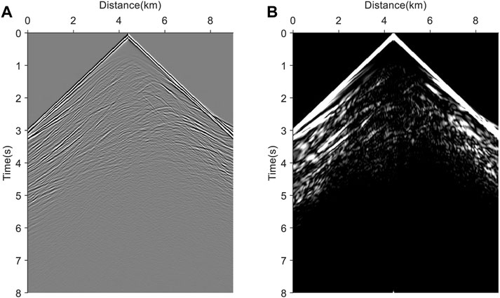
FIGURE 1. A shot gather of X-component and its envelope. (A) X-component of a shot gather. (B) The envelope of (A).

FIGURE 2

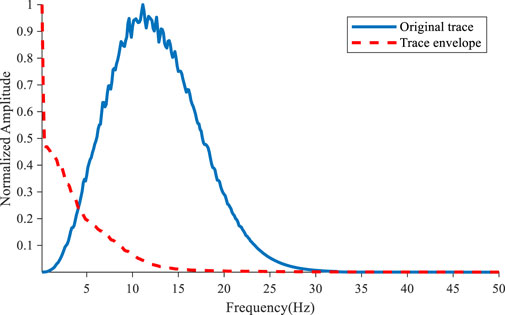
FIGURE 2. Normalized spectrum of Figures 1A, B.

In order to verify the low-frequency information extraction ability of the seismic data envelope, low-frequency components below 3 Hz were filtered out from seismic data, and the normalized spectra of low-frequency missing seismic data and their envelopes were obtained, as shown in Figure 3.

FIGURE 3

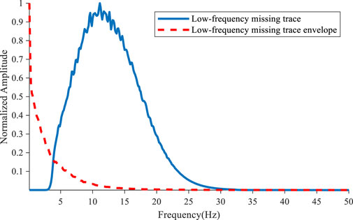
FIGURE 3. Normalized spectrum of low-frequency missing seismic data and their envelopes.

From Figure 3, it can be seen that although low-frequency information is missing from the seismic data, their envelope still contains rich low-frequency components. Therefore, seismic data envelopes based on Hilbert transform have the ability to extract low-frequency information.

Furthermore, the misfit function of elastic wave envelope inversion based on Hilbert transform can be defined as:

$J_{el}\left(\mathbf{m}\right)={\displaystyle \sum _{i=1}^{Ns}}{\displaystyle \sum _{j=1}^{Nr}}{\int }_0^{T_{\mathit{max}}}{\left[{\mathbf{D}}_{{\mathbf{u}}_{i,j}}^p-{\mathbf{D}}_{{\mathbf{d}}_{i,j}}^p\right]}^{2}dt,(13)$

where $T_{\mathit{max}}$ is the record length and ${\mathbf{D}}_{{\mathbf{u}}_{i,j}}^p$ and ${\mathbf{D}}_{{\mathbf{d}}_{i,j}}^p$ are the pth power of the vector envelope of the modeled and observed data, respectively.

In the two-dimensional case, there are:

${\left(D_{u_{i,j}^n}\right)}^p={\left\{{\left(u_{i,j}^n\right)}^2+\left[H{\left(u_{i,j}^n\right)}^2\right]\right\}}^{\frac{p}{2}}\left(n=x,z\right),(\mathrm{14a})$

${\left(D_{d_{i,j}^n}\right)}^p={\left\{{\left(d_{i,j}^n\right)}^2+\left[H{\left(d_{i,j}^n\right)}^2\right]\right\}}^{\frac{p}{2}}\left(n=x,z\right),(\mathrm{14b})$

where $D_{u_{i,j}^x}$ and $D_{u_{i,j}^z}$ are the envelope of the X and Z components of the modeled data, respectively, $D_{d_{i,j}^x}$ and $D_{d_{i,j}^z}$ are the envelope of the X and Z components of the observed data, respectively, $u_{i,j}^x$ and $u_{i,j}^z$ are the X and Z components of the modeled data, respectively, $d_{i,j}^x$ and $d_{i,j}^z$ are the X and Z components of the observed data, respectively, $i$ is the shot index number, and $j$ is the channel index number.

It should be noted that the value of p has a significant impact on the accuracy of envelope inversion. Chi et al. (2014) compared and analyzed the results of envelope inversion under different p-values, and their analysis results showed that a decrease in p-values would weaken the energy of deep reflected waves, thereby increasing the envelope inversion error of deep stratum. We study the first and second envelope inversion methods for elastic waves when p is taken as 1 and 2, respectively.

The gradient of the misfit function $J_{el}$ over the model parameter $\mathbf{m}$ can be expressed as:

$\frac{\partial J_{el}}{\partial \mathbf{m}}=p{\displaystyle \sum _{i=1}^{Ns}}{\displaystyle \sum _{j=1}^{Nr}}{\int }_0^T\left\{\left[{\mathbf{D}}_{{\mathbf{u}}_{i,j}}^p-{\mathbf{D}}_{{\mathbf{d}}_{i,j}}^p\right]{\mathbf{D}}_{{\mathbf{u}}_{i,j}}^{p-2}{\mathbf{u}}_{i,j}-H\left\{\left[{\mathbf{D}}_{{\mathbf{u}}_{i,j}}^p-{\mathbf{D}}_{{\mathbf{d}}_{i,j}}^p\right]{\mathbf{D}}_{{\mathbf{u}}_{i,j}}^{p-2}H\left({\mathbf{u}}_{i,j}\right)\right\}\right\}\frac{\partial {\mathbf{u}}_{i,j}}{\partial \mathbf{m}}dt.(15)$

In order to compare the formal similarities and differences between the gradient formula of elastic wave envelope inversion and the gradient formula of full waveform elastic wave inversion in the conventional time domain, the partial derivative of Eq. 1 with respect to model parameter $\mathbf{m}$ can be obtained as follows:

$\frac{\partial E}{\partial \mathbf{m}}={\displaystyle \sum _{i=1}^{Ns}}{\displaystyle \sum _{j=1}^{Nr}}{\int }_0^T\left({\mathbf{u}}_{i,j}-{\mathbf{d}}_{i,j}\right)\frac{\partial {\mathbf{u}}_{i,j}}{\partial \mathbf{m}}dt.(16)$

Comparing Eq. 15 and Eq. 16, it can be seen that the gradient of elastic wave envelope inversion is consistent in form with the gradient of conventional time domain elastic wave full waveform inversion. Therefore, envelope inversion can be carried out according to the process of time domain EFWI. The difference between the two is that the accompanying source of elastic wave envelope inversion is a function related to the seismic data envelope (Eq. 17), Therefore, it is only necessary to replace the accompanying source of the FWI of elastic waves in the conventional time domain to achieve elastic wave envelope inversion.

${\mathbf{f}}_{i,j}^{el}=p\left\{\left[{\mathbf{D}}_{{\mathbf{u}}_{i,j}}^p-{\mathbf{D}}_{{\mathbf{d}}_{i,j}}^p\right]{\mathbf{D}}_{{\mathbf{u}}_{i,j}}^{p-2}{\mathbf{u}}_{i,j}-H\left\{\left[{\mathbf{D}}_{{\mathbf{u}}_{i,j}}^p-{\mathbf{D}}_{{\mathbf{d}}_{i,j}}^p\right]{\mathbf{D}}_{{\mathbf{u}}_{i,j}}^{p-2}H\left({\mathbf{u}}_{i,j}\right)\right\}\right\},(17)$

where ${\mathbf{f}}_{i,j}^{el}$ is the accompanying source vector of the ith shot and the jth channel. In the two-dimensional case, there are:

$f_{i,j}^{el\left(x\right)}=p\left\{\left[{\left(D_{u_{i,j}^x}\right)}^p-{\left(D_{d_{i,j}^x}\right)}^p\right]{\left(D_{u_{i,j}^x}\right)}^{p-2}{u}_{i,j}^x-H\left\{\left[{\left(D_{u_{i,j}^x}\right)}^p-{\left(D_{d_{i,j}^x}\right)}^p\right]{\left(D_{u_{i,j}^x}\right)}^{p-2}H\left(u_{i,j}^x\right)\right\}\right\},(\mathrm{18a})$

$f_{i,j}^{el\left(z\right)}=p\left\{\left[{\left(D_{u_{i,j}^z}\right)}^p-{\left(D_{d_{i,j}^z}\right)}^p\right]{\left(D_{u_{i,j}^z}\right)}^{p-2}{u}_{i,j}^z-H\left\{\left[{\left(D_{u_{i,j}^z}\right)}^p-{\left(D_{d_{i,j}^z}\right)}^p\right]{\left(D_{u_{i,j}^z}\right)}^{p-2}H\left(u_{i,j}^z\right)\right\}\right\},(\mathrm{18b})$

where $f_{i,j}^{el\left(x\right)}$ and $f_{i,j}^{el\left(z\right)}$ are the X and Z components of ${\mathbf{f}}_{i,j}^{el}$.

4 Source-independent elastic wave envelope inversion

The elastic wave envelope inversion provided above is derived based on the assumption of accurate source wavelets, without considering the different effects of wavelets used in modeled wave fields and observed wave fields. In order to eliminate the influence of source wavelets on elastic wave envelope inversion, we extend the source-independent envelope inversion method to the field of elastic waves, so that the elastic wave envelope inversion can still establish a reliable initial model when the source wavelet is not accurate.

The misfit function of source-independent elastic wave envelope inversion can be expressed as:

$J_{cv1}\left(\mathbf{m}\right)=\frac{1}{2}{\displaystyle \sum _{i=1}^{Ns}}{\displaystyle \sum _{j=1}^{Nr}}{\int }_0^T\left[{\left({\mathbf{E}}_{cv\left(i,j\right)}^{\mathbf{u}}-{\mathbf{E}}_{cv\left(i,j\right)}^{\mathbf{d}}\right)}^2\right]dt,(19)$

where ${\mathbf{E}}_{cv\left(i,j\right)}^{\mathbf{u}}$ and ${\mathbf{E}}_{cv\left(i,j\right)}^{\mathbf{d}}$ are the envelope vectors of the modeled convolutional wave field and the observed convolutional wave field of the ith shot and the jth channel, respectively.

In the two-dimensional case, Eq. 19 can be written as:

$E_{cv\left(i,j\right)}^{u_x}=\sqrt{{\left(u_{i,j}^x*d_{i,k}^x\right)}^2+{\left[H\left(u_{i,j}^x*d_{i,k}^x\right)\right]}^2},(\mathrm{20a})$

$E_{cv\left(i,j\right)}^{u_z}=\sqrt{{\left(u_{i,j}^z*d_{i,k}^z\right)}^2+{\left[H\left(u_{i,j}^z*d_{i,k}^z\right)\right]}^2},(\mathrm{20b})$

$E_{cv\left(i,j\right)}^{d_x}=\sqrt{{\left(d_{i,j}^x*u_{i,k}^x\right)}^2+{\left[H\left(d_{i,j}^x*u_{i,k}^x\right)\right]}^2,}(\mathrm{20c})$

$E_{cv\left(i,j\right)}^{d_z}=\sqrt{{\left(d_{i,j}^z*u_{i,k}^z\right)}^2+{\left[H\left(d_{i,j}^z*u_{i,k}^z\right)\right]}^2}.(\mathrm{20d})$

It can be seen that the misfit function is composed of the sum of squares of the envelope residuals of the convolution wave fields in the x and z directions. Taking Eq. 20a and Eq. 20c as examples, the seismic wave field in the formula can be expressed in the form of Green’s function and source wavelet convolution, so Eq. 20a and Eq. 20c can be expressed as:

$E_{cv\left(i,j\right)}^{u_x}=\sqrt{{\left(u_{i,j}^x*d_{i,k}^x\right)}^2+{\left[H\left(u_{i,j}^x*d_{i,k}^x\right)\right]}^2}=\sqrt{{\left(g_{i,j}^{u^x}*g_{i,k}^{d^x}*s_i^{d^x}*s_i^{u^x}\right)}^2+{\left[H\left(g_{i,j}^{u^x}*g_{i,k}^{d^x}*s_i^{d^x}*s_i^{u^x}\right)\right]}^2},(20e)$

$E_{cv\left(i,j\right)}^{d_x}=\sqrt{{\left(d_{i,j}^x*u_{i,k}^x\right)}^2+{\left[H\left(d_{i,j}^x*u_{i,k}^x\right)\right]}^2}=\sqrt{{\left(g_{i,j}^{d^x}*g_{i,k}^{u^x}*s_i^{d^x}*s_i^{u^x}\right)}^2+{\left[H\left(g_{i,j}^{d^x}*g_{i,k}^{u^x}*s_i^{d^x}*s_i^{u^x}\right)\right]}^2.}(\mathrm{20f})$

In equations Eq. 20e and Eq. 20f, the simulated convolutional wave field envelope $E_{cv}^{u_x}$ and the observed convolutional wave field envelope $E_{cv}^{d_x}$ have the same source wavelet $s_i^{d^x}*s_i^{u^x}$. Similarly, both $E_{cv}^{u_z}$ and $E_{cv}^{d_z}$ have the same source wavelet $s_i^{d^z}*s_i^{u^z}$. Therefore, inversion based on the objective function $J_{cv1}$ can eliminate the influence of source wavelets on elastic wave envelope inversion.

The derivative of the misfit function $J_{cv1}$ over the model parameter $\mathbf{m}$ can be expressed as:

$\frac{\partial J_{cv1}}{\partial \mathbf{m}}={\displaystyle \sum _{i=1}^{Ns}}{\displaystyle \sum _{j=1}^{Nr}}{\int }_0^T\left({\mathbf{E}}_{cv\left(i,j\right)}^{\mathbf{u}}-{\mathbf{E}}_{cv\left(i,j\right)}^{\mathbf{d}}\right)\left(\frac{\partial {\mathbf{E}}_{cv\left(i,j\right)}^{\mathbf{u}}}{\partial \mathbf{m}}-\frac{\partial {\mathbf{E}}_{cv\left(i,j\right)}^{\mathbf{d}}}{\partial \mathbf{m}}\right)dt.(21)$

Since the observed convolution wave field contains the modeled reference trace wave field, its partial derivative to the model parameters is not zero, so Eq. 21 can be expanded to:

$\begin{array}{ll}\hfill \frac{\partial J_{cv1}}{\partial \mathbf{m}}& ={\displaystyle \sum _{i=1}^{Ns}}{\displaystyle \sum _{j=1}^{Nr}}{\int }_0^T\left\{\left({\mathbf{E}}_{cv\left(i,j\right)}^{\mathbf{u}}-{\mathbf{E}}_{cv\left(i,j\right)}^{\mathbf{d}}\right)\frac{1}{{\mathbf{E}}_{cv\left(i,j\right)}^{\mathbf{u}}}\left\{\left({\mathbf{u}}_{i,j}*{\mathbf{d}}_{i,k}\right)\left({\mathbf{d}}_{i,k}*\frac{\partial {\mathbf{u}}_{i,j}}{\partial \mathbf{m}}\right)+\left[H\left({\mathbf{u}}_{i,j}*{\mathbf{d}}_{i,k}\right)\left(H*{\mathbf{d}}_{i,k}*\frac{\partial {\mathbf{u}}_{i,j}}{\partial \mathbf{m}}\right)\right]\right.\}\right.\}dt\hfill \\ \hfill & -{\displaystyle \sum _{i=1}^{Ns}}{\displaystyle \sum _{j=1}^{Nr}}{\int }_0^T\left\{\left({\mathbf{E}}_{cv\left(i,j\right)}^{\mathbf{u}}-{\mathbf{E}}_{cv\left(i,j\right)}^{\mathbf{d}}\right)\frac{1}{{\mathbf{E}}_{cv\left(i,j\right)}^{\mathbf{d}}}\left\{\left({\mathbf{d}}_{i,j}*{\mathbf{u}}_{i,k}\right)\left({\mathbf{d}}_{i,j}*\frac{\partial {\mathbf{u}}_{i,k}}{\partial \mathbf{m}}\right)+\left[H\left({\mathbf{d}}_{i,j}*{\mathbf{u}}_{i,k}\right)\left(H*{\mathbf{d}}_{i,j}*\frac{\partial {\mathbf{u}}_{i,k}}{\partial \mathbf{m}}\right)\right]\right.\}\right.\}dt.\hfill \end{array}(22)$

According to Born’s approximation and convolution theorem (Choi et al., 2011), Eq. 22 can be transformed into:

$\frac{\partial J_{cv1}}{\partial \mathbf{m}}={\displaystyle \sum _{i=1}^{Ns}}{\displaystyle \sum _{j=1}^{Nr}}\left\{{\int }_0^T{\mathbf{W}}_{i,\mathbf{x}}^{\mathbf{u}}\left(t\right)\left\{{\int }_0^T{\mathbf{g}}_{\mathbf{x},j}^{\mathbf{u}}\left(\tau -t\right)\bullet {\mathbf{f}}_{i,j}\left(\tau \right)d\tau \right\}dt\right\}+{\displaystyle \sum _{i=1}^{Ns}}{\displaystyle \sum _{j=1}^{Nr}}\left\{{\int }_0^T{\mathbf{W}}_{i,\mathbf{x}}^{\mathbf{u}}\left(t\right)\left\{{\int }_0^T{\mathbf{g}}_{\mathbf{x},k}^{\mathbf{u}}\left(\tau -t\right)\bullet {\mathbf{f}}_{i,k}\left(\tau \right)d\tau \right\}dt\right\},(23)$

where subscript $\mathbf{x}$ is the spatial position vector, ${\mathbf{W}}_{i,\mathbf{x}}^{\mathbf{u}}$ is the simulated multi-component wavefield of the ith shot, ${\mathbf{g}}_{\mathbf{x},j}^{\mathbf{u}}$ is the Green’s function of the up-going wave, ${\mathbf{f}}_{i,j}=\left(f_{i,j}^x,f_{i,j}^z\right)$ is the adjoint source vector of the ith shot and the jth channel, and ${\mathbf{f}}_{i,k}=\left(f_{i,k}^x,f_{i,k}^z\right)$ is the adjoint source vector of the ith shot and the kth channel. Their calculation formula is as follows:

$\left\{\begin{array}{c}{f}_{i,j}^x=d_{i,k}^x\otimes \left\{\left(E_{cv\left(i,j\right)}^{u_x}-E_{cv\left(i,j\right)}^{d_x}\right)\frac{1}{E_{cv\left(i,j\right)}^{u_x}}\left(u_{i,j}^x*d_{i,k}^x\right)-H\left[\left(E_{cv\left(i,j\right)}^{u_x}-E_{cv\left(i,j\right)}^{d_x}\right)\frac{1}{E_{cv\left(i,j\right)}^{u_x}}H\left(u_{i,j}^x*d_{i,k}^x\right)\right]\right\},\\ f_{i,j}^z=d_{i,k}^z\otimes \left\{\left(E_{cv\left(i,j\right)}^{u_z}-E_{cv\left(i,j\right)}^{d_z}\right)\frac{1}{E_{cv\left(i,j\right)}^{u_z}}\left(u_{i,j}^z*d_{i,k}^z\right)-H\left[\left(E_{cv\left(i,j\right)}^{u_z}-E_{cv\left(i,j\right)}^{d_z}\right)\frac{1}{E_{cv\left(i,j\right)}^{u_z}}H\left(u_{i,j}^z*d_{i,k}^z\right)\right]\right\},\\ \begin{array}{c}{f}_{i,k}^x=-d_{i,j}^x\otimes \left\{\left(E_{cv\left(i,j\right)}^{u_x}-E_{cv\left(i,j\right)}^{d_x}\right)\frac{1}{E_{cv\left(i,j\right)}^{d_x}}\left(d_{i,j}^x*u_{i,k}^x\right)-H\left[\left(E_{cv\left(i,j\right)}^{u_x}-E_{cv\left(i,j\right)}^{d_x}\right)\frac{1}{E_{cv\left(i,j\right)}^{d_x}}H\left(d_{i,j}^x*u_{i,k}^x\right)\right]\right\},\\ f_{i,k}^z={-d}_{i,j}^z\otimes \left\{\left(E_{cv\left(i,j\right)}^{u_z}-E_{cv\left(i,j\right)}^{d_z}\right)\frac{1}{E_{cv\left(i,j\right)}^{d_z}}\left(d_{i,j}^z*u_{i,k}^z\right)-H\left[\left(E_{cv\left(i,j\right)}^{u_z}-E_{cv\left(i,j\right)}^{d_z}\right)\frac{1}{E_{cv\left(i,j\right)}^{d_z}}H\left(d_{i,j}^z*u_{i,k}^z\right)\right]\right\},\end{array}\end{array}\right.(24)$

where $\otimes$ is the cross correlation operator, ${\int }_0^T{\mathbf{g}}_{\mathbf{x},j}^{\mathbf{u}}\left(\tau -t\right)\bullet {\mathbf{f}}_{i,j}\left(\tau \right)d\tau$ and ${\int }_0^T{\mathbf{g}}_{\mathbf{x},k}^{\mathbf{u}}\left(\tau -t\right)\bullet {\mathbf{f}}_{i,k}\left(\tau \right)d\tau$ are the adjoint wavefield of the jth channel obtained through ${\mathbf{f}}_{i,j}$ backpropagation and the adjoint wavefield of the reference channel obtained through ${\mathbf{f}}_{i,k}$ backpropagation, respectively.

Eq. 23 and Eq. 24 show that the partial derivative of the misfit function $J_{cv1}$ with respect to the model parameter $\mathbf{m}$ is still the cross correlation between the forward wavefield and the adjoint wavefield, which is consistent with the gradient formula of the EFWI in the time domain in form. Therefore, in actual inversion, only the adjoint source of the time domain EFWI needs to be replaced by Eq. 24 to obtain the reverse-time propagation wave field, then a zero delay cross correlation can be performed between the reverse-time propagation wavefield and the forward wavefield according to Eq. 19 to obtain the corresponding gradient.

Similarly, the misfit function of source-independent second-order elastic wave envelope inversion can be defined as:

$J_{cv2}\left(\mathbf{m}\right)=\frac{1}{2}{\displaystyle \sum _{i=1}^{Ns}}{\displaystyle \sum _{j=1}^{Nr}}{\int }_0^T{\left[{\left({\mathbf{E}}_{cv\left(i,j\right)}^{\mathbf{u}}\right)}^2-{\left({\mathbf{E}}_{cv\left(i,j\right)}^{\mathbf{d}}\right)}^2\right]}^{2}dt.(25)$

The derivative of $J_{cv2}$ with respect to $\mathbf{m}$ can be expressed as:

$\frac{\partial J_{cv2}}{\partial \mathbf{m}}={\displaystyle \sum _{i=1}^{Ns}}{\displaystyle \sum _{j=1}^{Nr}}{\int }_0^T\left\{\begin{array}{c}2\left[{\left({\mathbf{E}}_{cv}^{\mathbf{u}}\right)}^2-{\left({\mathbf{E}}_{cv}^{\mathbf{d}}\right)}^2\right]\left\{\left({\mathbf{u}}_{i,j}*{\mathbf{d}}_{i,k}\right)\left({\mathbf{d}}_{i,k}*\frac{\partial {\mathbf{u}}_{i,j}}{\partial \mathbf{m}}\right)+2\left[H\left({\mathbf{u}}_{i,j}*{\mathbf{d}}_{i,k}\right)\left(H*{\mathbf{d}}_{i,k}*\frac{\partial {\mathbf{u}}_{i,j}}{\partial \mathbf{m}}\right)\right]\right\}\\ -2\left[{\left({\mathbf{E}}_{cv}^{\mathbf{u}}\right)}^2-{\left({\mathbf{E}}_{cv}^{\mathbf{d}}\right)}^2\right]\left\{\left({\mathbf{d}}_{i,j}*{\mathbf{u}}_{i,k}\right)\left({\mathbf{d}}_{i,j}*\frac{\partial {\mathbf{u}}_{i,k}}{\partial \mathbf{m}}\right)+2\left[H\left({\mathbf{d}}_{i,j}*{\mathbf{u}}_{i,k}\right)\left(H*{\mathbf{d}}_{i,j}*\frac{\partial {\mathbf{u}}_{i,k}}{\partial \mathbf{m}}\right)\right]\right\}\end{array}\right\}dt,(26)$

assuming that the adjoint source vectors of misfit function $J_{cv2}$ at receiver point j and reference channel k are ${\mathit{f}}_{i,j}^{\prime }$ and ${\mathit{f}}_{i,k}^{\prime }$, respectively. The adjoint source expression in vector form is as follows:

${\mathit{f}}_{i,j}^{\prime }={\mathbf{d}}_{i,k}\otimes \left\{2\left[{\left({\mathbf{E}}_{cv}^{\mathbf{u}}\right)}^2-{\left({\mathbf{E}}_{cv}^{\mathbf{d}}\right)}^2\right]\bullet \left({\mathbf{u}}_{i,j}*{\mathbf{d}}_{i,k}\right)-2H\left[\left[{\left({\mathbf{E}}_{cv}^{\mathbf{u}}\right)}^2-{\left({\mathbf{E}}_{cv}^{\mathbf{d}}\right)}^2\right]\bullet H\left({\mathbf{u}}_{i,j}*{\mathbf{d}}_{i,k}\right)\right]\right.\},(\mathrm{27a})$

${\mathit{f}}_{i,k}^{\prime }=-{\mathbf{d}}_{i,j}\otimes \left\{2\left[{\left({\mathbf{E}}_{cv}^{\mathbf{u}}\right)}^2-{\left({\mathbf{E}}_{cv}^{\mathbf{d}}\right)}^2\right]\bullet \left({\mathbf{d}}_{i,j}*{\mathbf{u}}_{i,k}\right)-2H\left[\left[{\left({\mathbf{E}}_{cv}^{\mathbf{u}}\right)}^2-{\left({\mathbf{E}}_{cv}^{\mathbf{d}}\right)}^2\right]\bullet H\left({\mathbf{d}}_{i,j}*{\mathbf{u}}_{i,k}\right)\right]\right.\}.(\mathrm{27b})$

So far, the gradient and adjoint source formulas for the first and second-order envelope inversion of elastic waves independent of wavelets have been obtained.

In terms of inversion strategy, Wang et al. (2016) proposed a multi-step multi-scale strategy for the reconstruction of high-accuracy P- and S-wave velocities, which uses envelope-based EFWI as the first step to obtain the long wavelength components of P- and S-wave velocities, and then uses the above velocities as initial models to obtain the final inversion results through multi-scale inversion. Due to the more natural multi-scale framework of mixed domain EFWI, we combine source-independent elastic wave envelope inversion with source-independent mixed domain EFWI to form a step-by-step multiscale inversion strategy when the source wavelet is inaccurate. The specific process is as follows: firstly, the low-frequency model is obtained by using the first or second-order source-independent elastic wave envelope inversion; then, the above low-frequency mode is used to perform a mixed domain source-independent multi-scale EFWI, and the final inversion results of P- and S-wave velocities are obtained. Theoretically, the strategy can not only avoid the influence of wavelet inaccuracy on the conventional mixed domain EFWI but, on the other hand, using source-independent elastic wave envelope inversion to provide an initial model is beneficial for reducing the probability of EFWI falling into local extrema.

5 Synthetic examples

5.1 Source-independent first-order envelope inversion test

We tested the performance of conventional envelope inversion and source-independent envelope inversion when the wavelet is inaccurate. Firstly, we used an incorrect wavelet to perform envelope inversion using both the above methods to obtain the low-frequency components of the P-and S-wave velocities; then, we used the source-independent EFWI to reconstruct the detailed information in the P- and S-wave velocity model.

The dataset used for testing was a two-component dataset obtained by a finite difference scheme of elastic wave equations on the model shown in Figures 4A, B, and the source wavelet used for simulation was a Ricker wavelet with a dominant frequency of 8 Hz. The model parameters and geometry of simulation were as follows: the space size of the model was 9,000 m × 3,500 m, and the grid size for simulation was 20 m × 20 m; the shot spacing was 200 m, the starting position of the first shot was 0 m, and a total of 45 shots were received in a full array; a total of 45 two-component shot gathers were simulated; all receivers were fixed and stationary, with 450 receivers uniformly placed on the surface, with a time sampling interval of 2 m and a recording length of 8s.

FIGURE 4

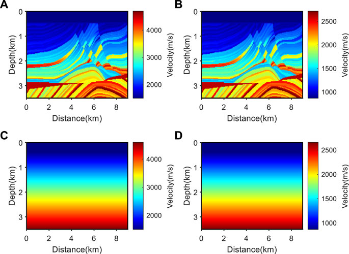
FIGURE 4. The real velocity model used for generating synthetic gathers and the initial velocity model used for envelope inversion. (A) Real P-wave velocity; (B) real S-wave velocity; (C) initial P-wave velocity; (D) initial S-wave velocity.

The wavelet used in the envelope inversion was the Ricker wavelet with a dominant frequency of 3 Hz. Before envelope inversion, a high-pass filtering of 0–5 Hz was performed on the two-component data to remove the low-frequency components in the input shot gathers, and the number of iterations in both the conventional envelope inversion and source-independent envelope inversion was 30. The initial velocity model used for envelope inversion is shown in Figures 5C, D. In the second stage, the source-independent EFWI adopts the frequency group configuration shown in Table 1, with a maximum of 20 iterations per frequency group. The source-independent inversion method selects the minimum offset trace of each shot as the reference channel.

FIGURE 5

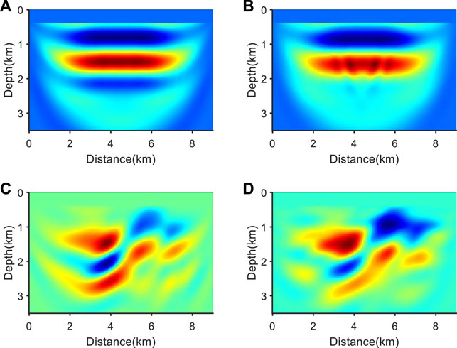
FIGURE 5. Gradient obtained from first-order envelope inversion based on an incorrect wavelet. (A) Gradient of P-wave velocity obtained from conventional envelope inversion; (B) gradient of S-wave velocity obtained from conventional envelope inversion; (C) gradient of P-wave velocity obtained from the source-independent envelope inversion; (D) gradient of S-wave velocity obtained from the source-independent envelope inversion.

TABLE 1

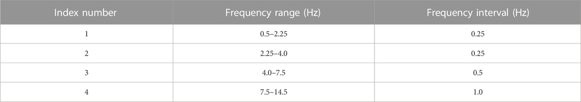
TABLE 1. Frequency group configuration for multi-scale EFWI.

In the iterative process of EFWI, it is first necessary to obtain the gradient, then use optimization algorithms to optimize the gradient, and finally achieve model update iteration with appropriate update steps. This indicates that whether the gradient can be correctly calculated directly determines the quality of the full waveform inversion results. Figure 5 shows the gradients obtained from conventional envelope inversion and source-independent envelope inversion when using incorrect wavelets. It is not difficult to see that the conventional envelope inversion shown in Figures 5A, B resulted in an error in obtaining the gradient in the case of incorrect wavelets. The use of this gradient for iterative model updates ultimately led to inversion failure (as shown in Figures 6A, B), while the gradient of the source-independent envelope inversion shown in Figures 5C, D correctly reflected the gradient information of large-scale structures. Therefore, it is possible to stably iterate and update the large-scale structures in the model (as shown in Figures 6C, D).

FIGURE 6

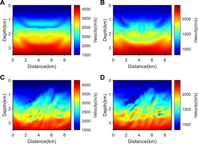
FIGURE 6. First-order envelope inversion results based on error wavelet. (A) P-wave velocity model obtained from conventional first-order envelope inversion; (B) S-wave velocity model obtained from conventional first-order envelope inversion; (C) P-wave velocity model obtained from source-independent first-order envelope inversion; (D) S-wave velocity model obtained from source-independent first-order envelope inversion.

From the inversion results shown in Figure 6, it can be seen that conventional envelope inversion is affected by incorrect wavelets and cannot accurately reconstruct the structural information of the model; the source-independent first-order envelope inversion eliminates the influence of wavelet differences through the convolution method, and the large-scale construction in the model is effectively restored. Figure 7 shows the decline curves of the normalized misfit function values for 30 iterations of two envelope inversion methods. It can be seen that the normalized misfit function values of conventional envelope inversion have almost no change when wavelet is inaccurate, while the misfit function values of source-independent envelope inversion decrease significantly. This indicates that source-independent envelope inversion can converge normally when wavelet errors occur, proving the correctness and effectiveness of the algorithm.

FIGURE 7

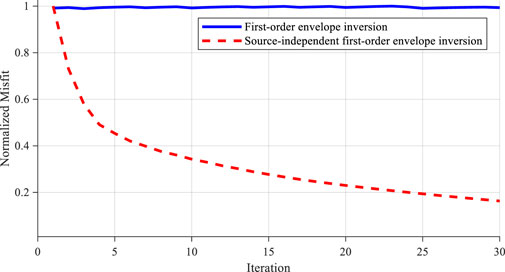
FIGURE 7. Comparison of normalized misfit function values for different inversion methods when the wavelet is inaccurate.

Furthermore, the source-independent EFWI was performed using the inversion results shown in Figures 6A–D, respectively. The results obtained are shown in Figures 8A–D.

FIGURE 8

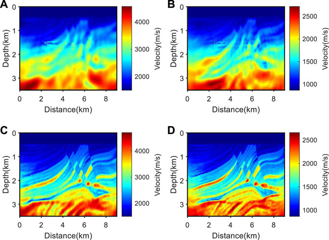
FIGURE 8. Source-independent EFWI results under two initial model conditions. (A) P-wave velocity model obtained from source-independent EFWI using Figures 6A, B as the initial model; (B) S-wave velocity model obtained from source-independent EFWI using Figures 6A, B as the initial model; (C) P-wave velocity model obtained from source-independent EFWI using Figures 6C, D as the initial model; (D) S-wave velocity model obtained from source-independent EFWI using Figures 6C, D as the initial model.

From Figure 8, it can be seen that when the wavelet is inaccurate, if the conventional first-order envelope inversion result is used as the initial model, the source-independent EFWI cannot obtain accurate inversion results. This is because the error information in the conventional first-order envelope inversion result causes the source-independent EFWI fall into local extrema, leading to inversion failure. While using the first-order source-independent envelope inversion result as the initial model for source-independent EFWI, the final inversion result shows clearer stratigraphic information and significantly better overall performance than the former. This indicates that when the wavelet is inaccurate, the first-order source-independent envelope inversion can accurately construct the long wavelength components in the P- and S-wave velocity model, thus aiding the full waveform inversion of elastic waves to obtain high-precision P- and S-wave velocity models.

5.2 Source-independent second-order envelope inversion test

The following tests were conducted for conventional and source-independent second-order envelope inversion when the wavelet is inaccurate. Figure 9 shows the gradient obtained through one iteration of conventional and source-independent second-order envelope inversion when the source wavelet is inaccurate.

FIGURE 9

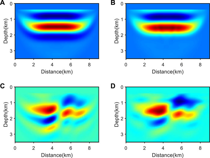
FIGURE 9. Gradient obtained from second-order envelope inversion based on error wavelet. (A) Gradient of P-wave velocity obtained from conventional second-order envelope inversion; (B) gradient of S-wave velocity obtained from conventional second-order envelope inversion; (C) gradient of P-wave velocity obtained from source-independent second-order envelope inversion; (D) gradient of S-wave velocity obtained from source-independent second-order envelope inversion.

Figure 9 shows that conventional second-order envelope inversion also experiences gradient estimation errors when wavelet errors occur, while source-independent second-order envelope inversion can correctly obtain gradient information of large-scale structures.

Figure 10 shows the conventional and source-independent second-order envelope inversion results when the inversion wavelet is inconsistent with the accurate wavelet. Figures 10A, B indicate that the conventional second-order envelope inversion results cannot reconstruct accurate initial velocity models of P- and S-waves when wavelet errors occur. On the contrary, the source-independent second-order envelope inversion has successfully constructed a low-frequency model containing large-scale information. Figure 11 shows the normalized misfit function values of conventional second-order envelope inversion and source-independent second-order envelope inversion when the source wavelet is inaccurate. We can see that the normalized misfit function values of conventional second-order envelope inversion have almost no change, indicating that the algorithm cannot converge normally, while the normalized misfit function values of source-independent second-order envelope inversion have significantly decreased, indicating that the algorithm can converge normally and proving the correctness and effectiveness of the algorithm proposed in this paper.

FIGURE 10

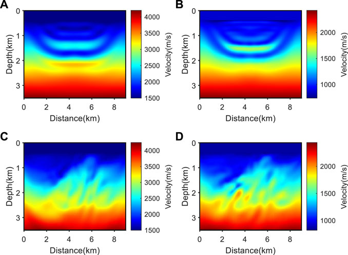
FIGURE 10. Second-order envelope inversion results based on error wavelet. (A) P-wave velocity model obtained from conventional second-order envelope inversion; (B) S-wave velocity model obtained from conventional second-order envelope inversion; (C) P-wave velocity model obtained from source-independent second-order envelope inversion; (D) S-wave velocity model obtained from source-independent second-order envelope inversion.

FIGURE 11

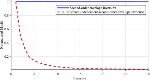
FIGURE 11. Comparison of normalized misfit function values for different inversion methods when the wavelet is inaccurate.

Using Figures 10A–D as initial models for source-independent EFWI, the results obtained are shown in Figure 12.

FIGURE 12

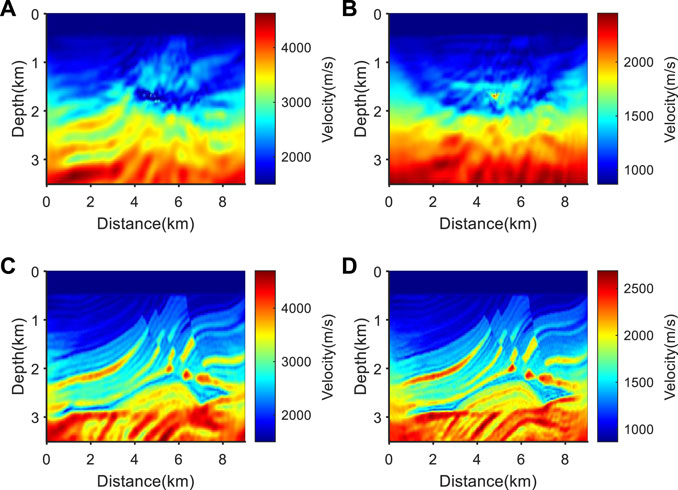
FIGURE 12. Source-independent EFWI results under different models. (A) P-wave velocity model obtained from source-independent EFWI using Figures 11A, B as initial model; (B) S-wave velocity model obtained from source-independent EFWI using Figures 11A, B as initial model; (C) P-wave velocity model obtained from source-independent EFWI using Figures 11C, D as initial model; (D) S-wave velocity model obtained from source-independent EFWI using Figures 11C, D as initial model.

From Figures 12A, B, it can be seen that when the wavelet is inaccurate, using the conventional second-order envelope inversion result as the initial velocity model for source-independent EFWI, there is almost no available structural information in the inversion results, so the inversion has failed. Using the source-independent second-order envelope inversion results shown in Figure 12C and Figure 12D as the initial model, and then conducting source-independent EFWI, the overall structure in the inversion results was well reconstructed, and the stratigraphic interface was depicted more clearly. This indicates that when the wavelet is inaccurate, source-independent second-order envelope inversion can effectively recover the long wavelength components of the model, helping to obtain high-precision P- and S-wave velocity models for EFWI.

5.3 Source-independent elastic wave envelope inversion test for low-frequency missing data

The following analysis shows the performance of source-independent elastic wave envelope inversion in cases of wavelet errors and missing low-frequency information. The low-frequency part of 0∼3 Hz from the two components shot gathers are filtered out to obtain low-frequency missing seismic records. Taking the X-component as an example, one of the seismic gather and its spectra before and after filtering are shown in Figure 13 and Figure 14, respectively. It can be clearly seen from Figure 14 that the low-frequency components of 0∼3 Hz in the seismic data have been filtered out.

FIGURE 13

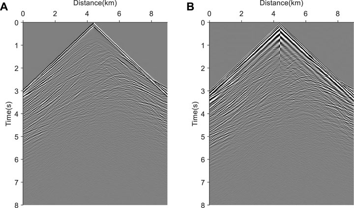
FIGURE 13. One of the X-component shot gather before and after filtering. (A) Original X-component shot gather; (B) X-component shot gather after a high pass filter.

FIGURE 14

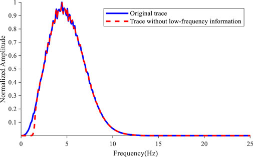
FIGURE 14. Spectra of X-component shot gather before and after high pass filtering.

Due to frequency band limitations, the starting frequency for mixed domain multiscale EFWI is 3 Hz. The specific frequency group configuration is shown in Table 2, and the maximum number of iterations for each frequency group is 20. The theoretical wavelet used in the test is a Ricker wavelet with a dominant frequency of 8 Hz. The error wavelet is a Ricker wavelet with a dominant frequency of 3 Hz.

TABLE 2

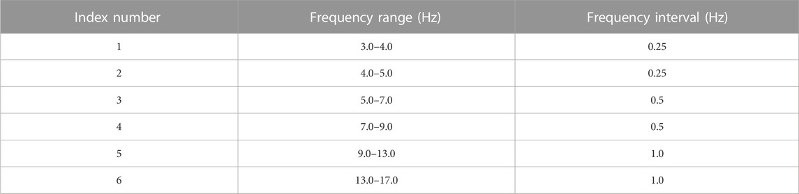
TABLE 2. Frequency group configuration for multi-scale EFWI for low-frequency missing data.

Firstly, conventional multiscale EFWI was performed, and the final results are shown in Figure 15. It can be seen that in the case of wavelet errors and missing low-frequency information, conventional EFWI cannot reconstruct the structural information of the model accurately, so inversion is unsuccessful.

FIGURE 15

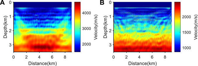
FIGURE 15. Conventional EFWI inversion results in cases of wavelet errors and missing low-frequency data. (A) P-wave velocity obtain form conventional EFWI; (B) S-wave velocity obtain form conventional EFWI.

Next, a source-independent EFWI test was conducted, and the results obtained are shown in Figure 16. It can be seen that the inversion accuracy of source-independent EFWI is improved compared to conventional EFWI. This is because source-independent EFWI uses the convolution method to eliminate the influence of incorrect wavelets, thus enabling stable inversion. However, for low-frequency missing data, the source-independent EFWI still shows a strong dependence on the initial model, with obvious velocity misestimation appearing in the red dashed area, and inversion falling into local minima.

FIGURE 16

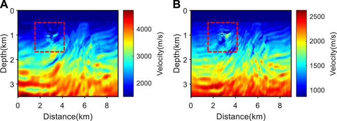
FIGURE 16. Source-independent EFWI results in cases of wavelet errors and missing low-frequency data. (A) P-wave velocity; (B) S-wave velocity.

To reduce inversion errors, we used source-independent first-order envelope inversion to establish a low-frequency initial model. The number of iterations for envelope inversion was 30, and the minimum offset trace of each shot was selected as the reference trace. Figure 17 shows the results of first-order source-independent envelope inversion. The inversion results show that the large-scale structure of the model has been correctly reconstructed, indicating that the method proposed in this paper can establish a good initial model in the absence of low-frequency data and inaccurate wavelets.

FIGURE 17

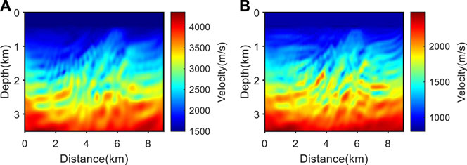
FIGURE 17. Source-independent first-order envelope inversion results in cases of wavelet errors and missing low-frequency data. (A) P-wave velocity; (B) S-wave velocity.

Using Figure 17 as the initial models for source-independent EFWI, the maximum number of iterations for each frequency group was set at 20, and the minimum offset trace of each shot was selected as the reference trace. Figure 18 shows the inversion results. It can be seen that there is no velocity estimation error in the red dashed box, which indicates that the initial model provided by the source-independent first-order envelope inversion alleviates the phenomenon of “cycle skipping".

FIGURE 18

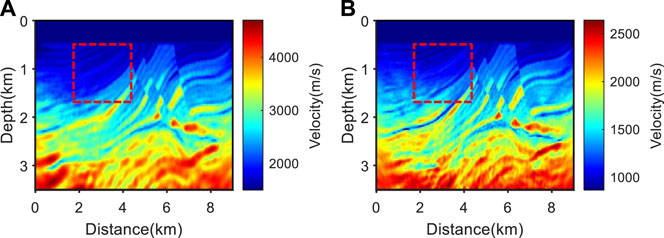
FIGURE 18. Results of source-independent EFWI using Figure 17 as the initial models. (A) P-wave velocity; (B) S-wave velocity.

Based on the same two-component low-frequency missing shot gathers, source-independent second-order envelope inversion was performed, and the inversion results were used as the initial model for source-independent EFWI. Figure 19 shows the initial model obtained from source-independent second-order envelope inversion. From Figure 19, it can be seen that the large-scale construction in the inversion results has also been effectively restored. Using Figure 19 as the initial model for source-independent EFWI, the final result is shown in Figure 20.

FIGURE 19

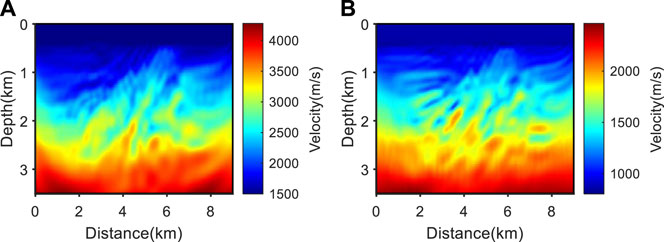
FIGURE 19. Source-independent second-order envelope inversion results in cases of wavelet errors and missing low-frequency data. (A) P-wave velocity; (B) S-wave velocity.

FIGURE 20

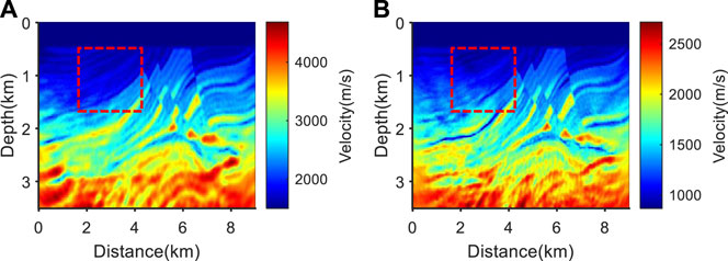
FIGURE 20. Results of source-independent EFWI using Figure 19 as the initial models. (A) P-wave velocity; (B) S-wave velocity.

Comparing Figure 16 and Figure 20 show that, compared to only performing source-independent EFWI, there are no velocity errors in the combined inversion results of source-independent second-order envelope inversion and source-independent EFWI. This indicates that the initial model provided by source-independent second-order envelope inversion can also alleviate the impact of the “cycle skipping” phenomenon. In addition, it should also be noted that the inversion accuracy of deep strata in the inversion results is relatively low, which will be a further research direction in the future.

6 Discussion

Our goal is to develop a depth domain P- and S-wave interval velocity models building method utilizing common shot gathers of multi-component seismic data. However, it is important to note that our current tests were conducted solely on synthetic data. Given the substantial disparities between synthetic and field data, it is crucial to exercise caution when applying this algorithm to real-world scenarios to address practical problems. The following data processing should be considered when working with field data:

(1) Preprocessing of multi-component seismic data (including denoising and surface consistency processing). The assumption in the algorithm we proposed assumes that the input multi-component seismic data do not contain noise and satisfy the assumption of surface consistency, while field data often do not meet above assumptions. Therefore, before using these algorithms for inversion of field data, it is necessary to perform noise suppression and surface consistency processing on the multi-component shot gathers to ensure that the input data are as close as possible to the above assumptions.

(2) Regularized reconstruction of multi-component seismic data in common shot domain. Due to factors such as acquisition cost, acquisition environment, and other acquisition conditions, the distribution of receivers in multi-component seismic exploration is often uneven and irregular; especially in ocean bottom multi-component seismic exploration, the distribution of receivers is often very sparse, so such data do not meet the requirements of the continuous receiver wave field required by the method in the paper. At the same time, since we use the finite difference method for wave propagation, which requires that each receiver must be located on the corresponding grid point, but the field data often does not meet this requirement, it is necessary to reconstruct the shot gathers before inversion to ensure that the spatial sampling rate of the input data and the spatial distribution of the receivers meet the implicit assumptions of our algorithm.

Usually, preprocessed multi-component seismic gathers often lack low-frequency information, which is one of the reasons for the failure of existing EFWI. Therefore, we use Hilbert transform to compensate for the low-frequency information in multi-component seismic data. But we emphasize that the Hilbert transform does not create low-frequency information out of thin air, but rather utilizes existing high-frequency information to predict and supplement low-frequency components. Through Hilbert envelope transformation, we can extract phase information from the observed high-frequency signals and use this phase information to synthesize a complex signal that can fully describe the spectral characteristics of the original signal (including the missing low-frequency components in the original signal). This supplementary low-frequency information is not completely new; it is inferred and restored from existing high-frequency signals through mathematical methods such as frequency domain analysis and phase correction. Therefore, Hilbert envelope transform is a mathematical method that effectively utilizes existing information to infer missing signal components.

7 Conclusion

When low-frequency time-domain FWI of information is missing in the multi-component seismic data, the EFWI strongly relies on an accurate initial model. When the initial model is poor, the inversion is easily trapped in local extrema. Elastic wave envelope inversion can establish a good initial model when low-frequency information is missing, but when the wavelet is not accurate, elastic wave envelope inversion cannot perform normal velocity model construction. We introduce the convolution-based source-independent method in the field of acoustic FWI into the elastic wave envelope inversion. We derived the gradient and adjoint source formulas for the source-independent elastic wave envelope inversion, and formed a step-by-step inversion strategy by combining the source-independent elastic wave envelope inversion and the source-independent mixed domain EFWI. The model testing results indicate that the source-independent elastic wave envelope inversion method we proposed can establish a good low-frequency model for P- and S-waves when seismic data lacks low-frequency information and the source wavelet is not accurate. Using the low-frequency models as the initial models for source-independent EFWI can effectively alleviate the impact of the “cycle skipping” phenomenon on the accuracy of EFWI.

Data availability statement

The original contributions presented in the study are included in the article/Supplementary Material, further inquiries can be directed to the corresponding author.

Author contributions

FL: Writing–original draft. XL: Writing–review and editing. TR: Writing–review and editing. GM: Writing–review and editing. BH: Writing–review and editing. JW: Writing–review and editing.

Funding

The author(s) declare financial support was received for the research, authorship, and/or publication of this article. The research was financially supported by the CNOOC Research Project “Seismic imaging and reservoir characterization of diapir and affected zone based on OBN data” (CNOOC-KJ GJHXJSGG YF 2022-01). The funder was not involved in the study design, collection, analysis, interpretation of data, the writing of this article, or the decision to submit it for publication.

Conflict of interest

Authors FL, XL, TR, GM and JW were employed by CNOOC China Limited, Hainan Branch.

The remaining author declares that the research was conducted in the absence of any commercial or financial relationships that could be construed as a potential conflict of interest.

Publisher’s note

All claims expressed in this article are solely those of the authors and do not necessarily represent those of their affiliated organizations, or those of the publisher, the editors and the reviewers. Any product that may be evaluated in this article, or claim that may be made by its manufacturer, is not guaranteed or endorsed by the publisher.

References

Ao, R., Dong, L., and Chi, B. (2015). Source-independent envelope-based FWI to build an initial model. Chin. J. Geophys. 58 (6), 1998–2010. (in Chinese). doi:10.6038/cjg20150615

CrossRef Full Text | Google Scholar

Baeten, G., Maag, J. W. d., Plessix, R., Klaassen, Rini., Qureshi, T., Kleemeyer, M., et al. (2013). The use of low frequencies in a full-waveform inversion and impedance inversion land seismic case study. Geophys. Prospect. 61, 701–711. doi:10.1111/1365-2478.12010

CrossRef Full Text | Google Scholar

Boonyasiriwat, C., Valasek, P., Routh, P., Cao, W., Schuster, G. T., and Macy, Brian. (2009). An efficient multiscale method for time-domain waveform tomography. Geophysics 74 (6), WCC59–WCC68. doi:10.1190/1.3151869

CrossRef Full Text | Google Scholar

Bozdağ, E., Trampert, J., and Tromp, J. (2011). Misfit functions for full waveform inversion based on instantaneous phase and envelope measurements. Geophys. J. Int. 185 (2), 845–870. doi:10.1111/j.1365-246X.2011.04970.x

CrossRef Full Text | Google Scholar

Bunks, C., Saleck, F. M., Zaleski, S., and Chavent, G. (1995). Multiscale seismic waveform inversion. Geophysics 60 (5), 1457–1473. doi:10.1190/1.1443880

CrossRef Full Text | Google Scholar

Chen, G., Wu, R. S., and Chen, S. (2018). Reflection multi-scale envelope inversion. Geophys. Prospect 66, 1258–1271. doi:10.1111/1365-2478.12624

CrossRef Full Text | Google Scholar

Chi, B., Dong, L., and Liu, Y. (2014). Full waveform inversion method using envelope objective function without low frequency data. J. Appl. Geophy. 109, 36–46. doi:10.1016/j.jappgeo.2014.07.010

CrossRef Full Text | Google Scholar

Choi, Y., and Alkhalifah, T. (2011). Source-independent time-domain waveform inversion using convolved wavefields: application to the encoded multisource waveform inversion. Geophysics 76 (5), R125–R134. doi:10.1190/GEO2010-0210.1

CrossRef Full Text | Google Scholar

Choi, Y., Shin, C., Min, D., and Ha, T. (2005). Efficient calculation of the steepest descent direction for source-independent seismic waveform inversion: an amplitude approach. J. Comput. Phys. 208 (2), 455–468. doi:10.1016/j.jcp.2004.09.019

CrossRef Full Text | Google Scholar

Datta, D., and Sen, M. K. (2016). Estimating a starting model for full-waveform inversion using a global optimization method. Geophysics 81 (4), R211–R223. doi:10.1190/GEO2015-0339.1

CrossRef Full Text | Google Scholar

Hu, Y., Han, L., Xu, Z., and Zhang, T. (2017). Demodulation envelop multi-scale full waveform inversion based on precise seismic source function. Chin. J. Geophys. 60 (3), 1088–1105. (in Chinese). doi:10.6038/cjg20170321

CrossRef Full Text | Google Scholar

Huang, C., Dong, L., Liu, Y., and Chi, B. (2015). Elastic envelope inversion using multicomponent seismic data without low frequency. Appl. Geophys. 12, 362–377. doi:10.1190/FWI2015-013

CrossRef Full Text | Google Scholar

Jun, H., Kim, Y., Shin, J., Shin, C., and Min, D. (2014). Laplace-Fourier-domain elastic full-waveform inversion using time-domain modeling. Geophysics 79 (5), R195–R208. doi:10.1190/GEO2013-0283.1

CrossRef Full Text | Google Scholar

Kim, Y., Shin, H., Calandra, H., and Min, D. (2013). An algorithm for 3D acoustic time-Laplace-Fourier-domain hybrid full-waveform inversion. Geophysics 78 (4), R151–R166. doi:10.1190/GEO2012-0155.1

CrossRef Full Text | Google Scholar

Krebs, J. R., Anderson, J. E., Hinkley, D., Neelamani, N., Lee, S., Baumstein, A., et al. (2009). Fast full-wavefield seismic inversion using encoded sources. Geophysics 74 (6), WCC177–WCC188. doi:10.1190/1.3230502

CrossRef Full Text | Google Scholar

Lailly, P. (1983). “The seismic inverse problem as a sequence of before-stack migration,” in Conference on inverse scattering: Theory and application (Society for Industrial and Applied Mathematics), Aalborg, Denmark, July 3–7, 1983, 20–220.

Google Scholar

Lewis, W., Amazonas, D., Vigh, D., and Coates, R. (2014). “Geologically constrained full-waveform inversion using an anisotropic diffusion based regularization scheme: application to a 3d offshore brazil dataset,” in 84th Annual International Meeting, SEG, Expanded Abstracts, Denver, Colorado, 26-31 October 2014, 1083–1088.

Google Scholar

Liu, Y., Chen, G., Hu, L., Huang, Y., Chang, M., and Contrino, C. (2014). “Improving images below shallow gas clouds with adaptive data-selection FWI and Q-tomography: A case study at east breaks, gom,” in 84th Annual International Meeting, SEG, Expanded Abstracts, Denver, Colorado, 26-31 October 2014, 1099–1104.

Google Scholar

Pratt, R. G., and Worthington, M. H. (1990). Inverse theory applied to multi-source cross-hole tomography. Part 2: elastic wave-equation method. Geophys. Prospect. 38 (3), 311–329. doi:10.1111/j.1365-2478.1990.tb01847.x

CrossRef Full Text | Google Scholar

Sirgue, L., Barkved, O., Dellinger, J., Etgen, J., Albertin, U., and Kommedal, J. H. (2010). Thematic set: full waveform inversion: the next leap forward in imaging at valhall. First Break 28 (1), 65–70. doi:10.3997/1365-2397.2010012

CrossRef Full Text | Google Scholar

Song, Z., Williamson, P. R., and Pratt, R. G. (1995). Frequency-domain acoustic-wave modeling and inversion of crosshole data: part ii—inversion method, synthetic experiments and real-data results. Geophysics 60 (3), 796–809. doi:10.1190/1.1443818

CrossRef Full Text | Google Scholar

Tarantola, A. (1986). A strategy for nonlinear elastic inversion of seismic reflection data. Geophysics 51 (10), 1893–1903. doi:10.1190/1.1442046

CrossRef Full Text | Google Scholar

Tarantola, A. (1984). Inversion of seismic reflection data in the acoustic approximation. Geophysics 49 (8), 1259–1266. doi:10.1190/1.1441754

CrossRef Full Text | Google Scholar

Wang, B., Gao, J., Zhang, H., and Zhao, W. (2011). “CUDA-based acceleration of full waveform inversion on GPU,” in SEG technical program expanded abstracts (Texas, United States: SEG), 2528–2533. doi:10.1190/1.3627717

CrossRef Full Text | Google Scholar

Wang, Y., Dong, L., Huang, C., and Liu, Y. (2016). A multi-step strategy for mitigating severe nonlinearity in elastic full-waveform inversion. OGP 51 (2), 288–294. doi:10.13810/j.cnki.issn.1000-7210.2016.02.011

CrossRef Full Text | Google Scholar

Wu, R., Luo, J., and Wu, B. (2014). Seismic envelope inversion and modulation signal model. Geophysics 79 (3), WA13–WA24. doi:10.1190/GEO2013-0294.1

CrossRef Full Text | Google Scholar

Wu, R., Luo, J., and Wu, B. (2013). “Ultra-low-frequency information in seismic data and envelope inversion,” in 2013 SEG annual meeting (Houston, United States: Society of Exploration Geophysists). doi:10.1190/segam2013-0825.1

CrossRef Full Text | Google Scholar

Wu, R. S., and Chen, G. (2018). Multi-scale seismic envelope inversion using a direct envelope Fréchet derivative for strong-nonlinear full waveform inversion. Available at: https://arxiv.org/abs/1808.05275 (accessed November 20, 2022).

Google Scholar

Wu, R. S., and Chen, G. (2017). “New Fréchet derivative for envelope data and multi-scale envelope inversion,” in Proceedings of the 79th EAGE Annual Meeting, Paris, France, 12–15 June 2017.

Google Scholar

Wu, R. S. (2020). Towards a theoretical background for strong-scattering inversion—direct envelope inversion and gel’fand-LevitanMarchenko theory. Commun. Comput. Phys. 28, 41–73. doi:10.4208/cicp.oa-2018-0108

CrossRef Full Text | Google Scholar

Xu, K., and McMechan, G. A. (2014). 2D frequency-domain elastic full-waveform inversion using time-domain modeling and a multistep-length gradient approach. Geophysics 79 (2), R41–R53. doi:10.1190/GEO2013-0134.1

CrossRef Full Text | Google Scholar

Zhong, M., Tan, J., Song, P., Zhang, X., Xie, C., and Liu, Z. (2017). “Time-domain full waveform inversion using the gradient preconditioning based on seismic wave energy: application to the south china sea,” in CGS/SEG International Geophysical Conference: Geophysical challenges and prosperous development, Qingdao, China, April 17 to 20, 2017.

Google Scholar

Zhu, H. J., and Fomel, S. (2016). Building good starting models for full-waveform inversion using adaptive matching filtering misfit. Geophysics 81 (5), U61–U72. doi:10.1190/GEO2015-0596.1

CrossRef Full Text | Google Scholar