 Lili Zeng
 Weijian Ren1,2*
- 1Northeast Petroleum University, Daqing, China
- 2Heilongjiang Provincial Key Laboratory of Networking and Intelligent Control, Daqing, China
Reliable lithology spatial distribution directly reflects the geological situation of the reservoir, which is the basis of stratigraphic correlation, sedimentary modeling, and other geological research. Under the condition of limited reservoir data, it is a challenging task to accurately depict the lithology spatial distribution and provide a quantitative reliability analysis of the results. In this study, we propose a flexible spatial distribution prediction and model reliability analysis method. Firstly, the method develops a spatially dependent deep Kriging technology to fit the heterogeneous characteristics of the reservoir lithology, and adopts the extracted spatial key information and related reservoir attributes to invert lithology spatial distribution intelligently. Then, it focuses on the real-time assimilation of non-Gaussian data in the reliability modeling and quantitatively analyzes the reliability of the prediction system under the non-Gaussian hypothesis. Finally, the method is applied to the actual heterogeneous reservoir, good results are achieved in the prediction accuracy, model fitting degree, model reliability, and time performance compared with other methods. The method is conducive to finding future mineral deposits locations and reducing exploration costs.
1 Introduction
Kriging technology provides an optimal linear unbiased estimation of spatial interpolation and has an excellent performance in spatial information extraction (Zimmerman and Holland, 2005; Emery, 2008; Guo-Shun et al., 2010). The technology has already achieved notable results across geological science, biological science, and other fields (Gerstmann and Doktor, 2016; Erten et al., 2022), especially in spatial distribution prediction based on dense sample conditions (Du, 2020), which provides basic data for stratum model visualization.
Walvoort and Gruijter (2001) took the composition data as the research object, and fitted the spatial structure and non-negative constraints of the composition data well based on the combined Kriging technology. Korjani et al. (2006) combined fuzzy Kriging and deep learning to estimate reservoir lithology at any point in the field, which qualitatively captured the uncertainties associated with reservoir characteristics. Based on the Kriging technology and neural networks, Hansen et al. (2008) inverted the lithology distribution by using layer velocity, reflected layer roughness, and rock properties, with an accuracy close to that of actual exploration results.
Reservoir lithology is a typical component data (Zuo et al., 2013) with non-Gaussian and non-stationary characteristics. The distribution area is limited by certain geological conditions and constraints. The modeling of spatial distribution under Gaussian conditions is contrary to the actual geological idea. Furthermore, the maximum likelihood estimation under the multivariate Gaussian hypothesis involves the inverse operation of the positive definite covariance matrix (Heaton et al., 2018). The operation is usually Cholesky decomposition. The time complexity is
Deep learning has the ability to reveal nonlinear and non-stationary characteristics of complex structures (Airaudo et al., 2015; Zoltowska et al., 2021), which makes it extremely successful in spatiotemporal modeling tasks (Hauptmann et al., 2018; Suresha et al., 2020). Among them, models based on convolutional neural networks (CNN) have become a research hotspot. CNN captures the spatiotemporal features in the process of image processing through filters, and applies them to the image field, environmental field, and transportation field of massive data (Robert et al., 2018; Pak et al., 2020; Zhang et al., 2020). These methods are limited to images with regular grid cells and pay less attention to reservoir lithology distributions with irregular locations.
In particular, deep neural network (DNN) has the black-box characteristics (Montavon et al., 2016; Natekar et al., 2020; Qiao et al., 2021) during the training process of feature extraction by simulating human brain mechanisms, increasing model uncertainty. The uncertainty reduces the engineering applicability of the model (Janssen, 2013). Therefore, capturing uncertainty to achieve model reliability evaluation is a key step in prediction systems engineering applications. Under the condition of Gaussian distribution, some researchers obtained model reliability by capturing the uncertainty of the weights of the neural network (Pearl, 1990; MacKay, 1992; Gal and Ghahramani, 2015). However, in the training process of DNN, the weights changes with time and have the characteristics of random, dynamic, and non-Gaussian (Choi et al., 2018). Zeng (2021) et al. modeled the uncertainty of deep neural networks and quantitatively captured the uncertainty of logging data prediction results, effectively improving the engineering applicability of the model. The reliability analysis under the Gauss hypothesis will degrade the model performance, and even lead to the model not being able to work normally.
Aiming at the problems in reservoir prediction and reliability analysis modeling, this paper proposed a novel method for reservoir lithology spatial distribution prediction and reliability evaluation. Firstly, a spatial-dependent deep Kriging technology is developed to approximate the Kriging spatial correlation process and obtain spatial key information. Combined with the spatial key information and related reservoir attributes, the spatial distribution of heterogeneous reservoir lithology can be accurately and intelligently predicted based on deep learning. Secondly, the reliability of the prediction system is quantitatively evaluated under a non-Gaussian hypothesis by assimilating the non-Gaussian data in real-time. Finally, the method is applied to the laterite nickel ore heterogeneous reservoir, and evaluated from the prediction accuracy, model reliability, and time performance.
2 Methodology
2.1 Model design
Considering the Gaussian hypothesis problem existing in spatial distribution prediction and uncertainty analysis modeling, this section proposes a reservoir lithology spatial distribution prediction method based on deep learning technology (NG_GRU_Kriging). Its network architecture is shown in Figure 1. The NG_GRU_Kriging model is mainly composed of a feature extraction network and a reliability analysis network. The feature extraction network extracts the reservoir spatial feature by Spatial dependent deep Kriging technology and realizes the prediction of reservoir lithology spatial distribution. The reliability analysis network focuses on the non-Gaussian distribution characteristics of the weight parameters of the DNN_Bayes network, and adopts the GS_IENKF method to assimilate the non-Gaussian data in real time. It constructs the reliability evaluation system of the reservoir prediction system under the non-Gaussian hypothesis.
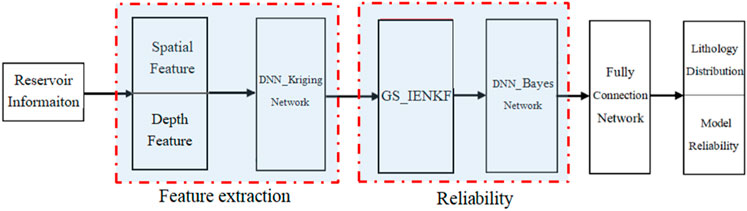
FIGURE 1. The network architecture of the NG_GRU_Kriging model.
In addition, the Kriging model and GRU_Kriging model are also constructed. The Kriging model directly takes the feature information extracted by the Kriging technology and reservoir depth features as the input of the reliability analysis network. Compared with the NG_GRU_Kriging model, the Kriging model and GRU_Kriging model are constructed under the Gaussian hypothesis.
2.2 Spatial-dependent deep kriging technology
2.2.1 Spatial key information extraction
Considering the spatial process
where
Aiming at the non-Gaussian characteristics of reservoir lithology, a log-ratio conversion module is constructed to make it approximately obey the Gaussian distribution. Eq. 2 is the conversion formula for lithology data (Odeh et al., 2013).
where
We seek several orthogonal radial basis functions to approximate the spatial correlation processes based on Karhunen Loeve theorem (Ogawa and Oja, 1986). The decomposition of the lithology spatial correlation process is determined by Eq. 3.
where,
For the spatial coordinates of reservoir lithology, we obtain relevant spatial key information by calculating orthogonal radial basis functions from lithology coordinates, as shown in Eq. 5. The approximate substitution avoids the problems of memory complexity and time complexity caused by the Cholesky decomposition.
In the same study area, different reservoir attributes at the same depth have different effects on the prediction accuracy. The depth feature of reservoir depth accumulation is extracted by adopting the logging depth feature attention module (Zeng et al., 2021), as shown in Eq. 66.
where
2.2.2 Spatial distribution prediction based on deep learning
The radial basis function is adopted to approximate the spatial correlation process before transferring the data to the hidden layer of DNN. Taking the joint key information
The extracted joint key information is embedded into the hidden layer of the deep neural network. Taking the GRU network as an example, the reset gate information is rewritten as Eq. 7. The reset gate can control the importance of the state information at the previous time, reducing the risk of gradient explosion and other problems (Cho et al., 2014).
Similarly, the new memory information
The update gate
The hidden layer state
In Eqs. 7–10,
Compared with classical technology, SDDK technology does not require any assumptions and can obtain more spatial key information by calculating multiple basis functions to approximate the spatial processes.
Finally, the fully connected neural network is adopted to linearly transform the comprehensive feature information. For the regression problems, Sigmoid is selected as the activation function. The result is determined by Eq. 11.
For the classification problems, Softmax is selected as the activation function. Eq. 12 gives the probability function (
The optimization objective function of the model consists of cross-entropy loss function and
where
2.3 Real-time assimilation of non-gaussian data
Combined with deep learning and Bayesian theory, the weights of DNN are modeled to obtain the reliability of the prediction system from the perspective of probability (Denker and Lecun, 1991). Given the reservoir data set (
where
An effective reservoir prediction system should be able to provide a reliability analysis of the results without being limited by Gaussian distribution and other hypotheses. In order to solve the problem of the Gaussian hypothesis in the reliability modeling, a Gaussian transform iterative Kalman filter (GS_IENKF) method is proposed based on the Kalman filtering principle (Gu and Oliver, 2007; Zhou et al., 2011). The data assimilation process of the GS_IENKF method is shown in Figure 2, the specific description is as follows.
(1) In the initial stage of the GS_IENKF method, the vector set
(2) Gaussian transform. Gaussian transform includes the transformation of the model vector and state vector. Firstly, the local cumulative probability distribution function is constructed (Ou et al., 1997). The extreme value of each state is defined in advance to prevent the updated vector from exceeding the probability distribution range. Then, the Gaussian transform equation is used to ensure the vector conforms to the univariate edge Gaussian distribution (Eq. 16).
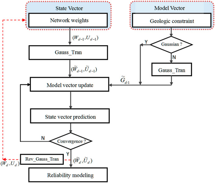
FIGURE 2. The flow chart of non-Gaussian data real-time assimilation (GS_IENKF).
The augmented matrix of the transformed model vector and state vector can be rewritten as Eq. 17.
where
The GS_IENKF method mainly completes the real-time assimilation of non-Gaussian data by updating the model vector and predicting the state vector.
(3) Model vector update. For the nonlinear reservoir lithology spatial distribution prediction system, a series of linear functions
The model vector and state vector satisfy a linear relationship approximately. The vector augmented matrix Eq. 18 can be written as Eq. 20.
The linear approximate covariance
The minimization objective function of the model vector is determined by Eq. 22.
In order to improve the adaptive ability of the deep learning model, automatic matching of iterative steps is realized through
where
(4) State vector prediction. Using the updated model parameters, the network weight parameter state of the state vector set is updated from state
where,
(5) If
(6) Return to step 2) to assimilate all the weight parameters of the deep neural network in real-time.
In the prediction process of heterogeneous reservoir data, the GS_IENKF method assimilates the output weights of the DNN network in real-time. Under the non-Gaussian hypothesis, the quantitative evaluation of the prediction system reliability is realized by combining with Bayesian theory, which can reduce the error cumulative effect caused by the non-Gaussian characteristics of the original distribution changed in the iteration process.
3 Case study in the actual work area
Combined with the heterogeneous reservoir of Australian laterite nickel ore, the spatial distribution prediction and reliability analysis of reservoir lithology are realized under the non-Gaussian hypothesis. The main contents of this section include the following. 1) The introduction of experimental parameters. 2) The data set description of the research area. 3) The prediction of reservoir lithology spatial distribution. 4) The evaluation of Model reliability. 5) Time analysis of the prediction model.
3.1 Experimental environment and operation settings
The experimental operating system is Windows 10, equipped with CPU version 12th Gen Intel R) Core (TM) i9-12900H, GPU NVIDIA GeForce RTX 3090, and deep learning framework Tenorflow2.4.0+cu110. The training dataset (80%) is used to train the prediction model, and the testing dataset (20%) is used to verify and evaluate the model performance. When the experimental training cycle is 40, the batches are 16, and the learning rate is 0.0001, the model performance reaches its optimal level. Meanwhile, Dropout technology and Adam optimizer are adopted to avoid model overfitting.
3.2 Data set
The laterite nickel ore data studied in this paper is collected from New South Wales, Australia, which belongs to the New England fold belt, extending in a north-south direction (Brand et al., 1998). The fold belt is dominated by marine facies, magmatic rocks, and metamorphic hydrothermal deposits. Nickel laterite is developed in the spherical profile of weathered lithology, and the rocks are enriched in the oxidation zone of the weathered layer. The spatial distribution of lithology is controlled by primary shear, resulting in discrete and steep cuttings along strike faults (Xu et al., 2013). The study area is dominated by mudstone and mud sandstone, mainly composed of chlorite, nontronite, and goethite. Nickel occurs in the latter two minerals with a content of about 1.5%–1.8%. It is also known as the transitional laterite nickel ore.
A total of 32,575 data samples from 1,200 wells in the study area were selected, including and 80% training set and a 20% test set. Table 1 shows the description of the test set. The related reservoir information longitude coordinate (long), latit coordinate (latit), multi-scale ridge flatness index (mrrtf), multi-scale valley flatness index (mrvb), topographic humidity index (twi), slope gradient (slope), and river channel distance (rdis) were utilized to achieve the prediction of lithology spatial distribution. The studied reservoir lithology mainly consists of clay (CLAY), sand (SAND), gravel (GRVL), shale (SHLE), sandstone (SDSN), and basalt (BALT).
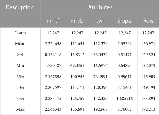
TABLE 1. The description of the test set.
Spearman correlation coefficient (SPCC) is applied to evaluate the relationship between the comprehensive lithology and related attributes. The lithology is weakly correlated with long, latit, mrrtf, and mrvb, with SPCCs of −0.39, 0.35, 0.29, 0.33, and 0.35, respectively. There is an extremely weak correlation between lithology and twi, slope, rdis, with SPCCs being 0.043, −0.1, and −0.0046, respectively.The weak relation creates some challenges for prediction.
The selected data were preprocessed to improve the accuracy of reservoir lithology prediction, including data cleaning, data outlier processing, and data normalization. Firstly, box graph theory was used for outlier detection and median substitution of the selected data to eliminate the influence of anomalous data on the prediction. Then, the least square polynomial fitting method was adopted to correct the replacement values according to the overall distribution trend of each attribute to ensure data stability. Finally, all the data in the study area were normalized to reduce the influence of errors caused by data calibration standards, data dimension, and maximum value on modeling accuracy of deep neural network.
3.3 The prediction of lithology spatial distribution
Table 2 presents the coefficient of determination (
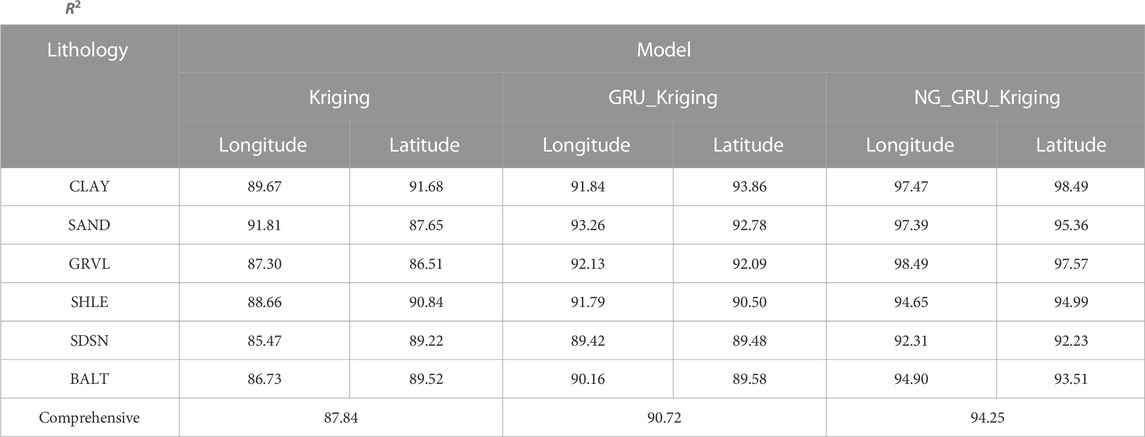
TABLE 2.
Under a non-Gaussian hypothesis, the NG_GRU_Kriging method adopts SDDK technology to extract more spatial key information, which is more in line with the actual geological conditions. This method accurately captures the spatial correlation reflecting the real reservoir lithology and effectively improves the prediction accuracy of single lithology spatial distribution. The accuracy of comprehensive lithology inverted results is 94.25%, which is 6.41% and 3.53% higher than the Kriging model and GRU_Kriging model, respectively.
Figure 3 shows the mean absolute percentage error (Mape) of the three models. Taking the average of the five experimental results, the Mape of Kriging, GRU_Kriging, and NG_GRU_Kriging models are 5.283%, 4.613%, and 3.505%, respectively. Thus, the performance of the proposed method is more stable.
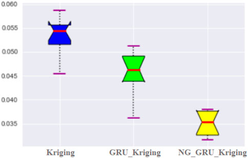
FIGURE 3. Comprehensive mean absolute percentage error in the models.
Figure 4 shows the actual lithology spatial distribution, and Figures 5–7 show the predicted results of the three models. Pearson correlation coefficient (PCC) is used to measure the linear fitting degree between the predicted and actual lithology distribution from the longitude and latitude directions. The linear fitting degree of lithology spatial distribution obtained by the Kriging method (Figure 4) is 92.7%. The situation is improved by 1.84% in the GRU_Kriging method (Figure 5). The RNN model can predict the approximate changed trend of reservoir lithology.
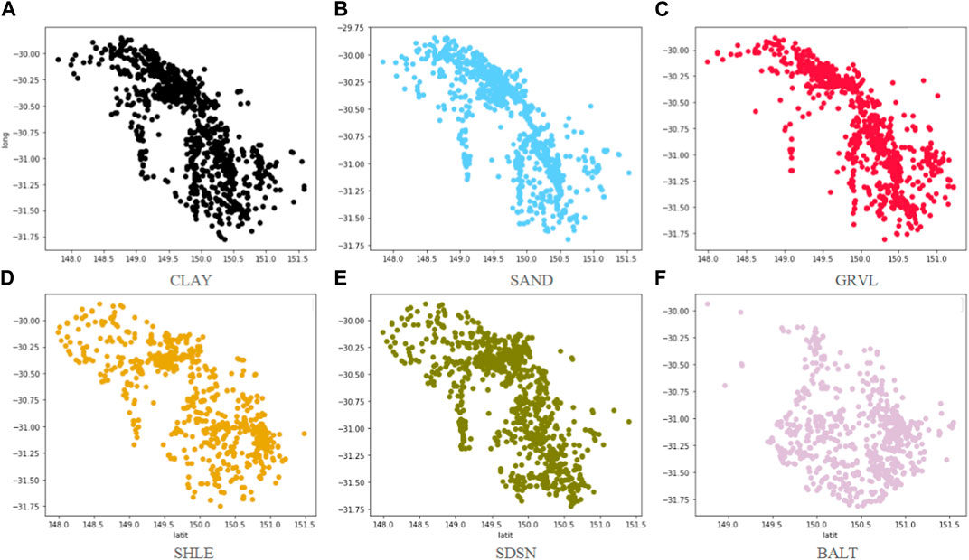
FIGURE 4. Actual lithology spatial distribution.
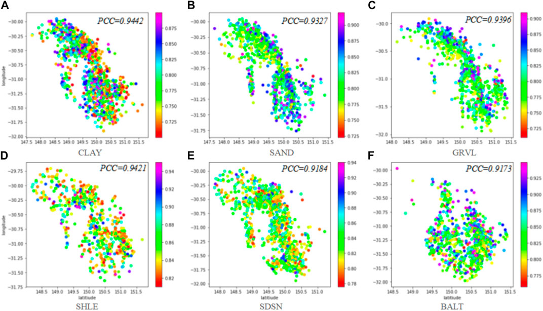
FIGURE 5. Lithology spatial distribution in the Kriging model.
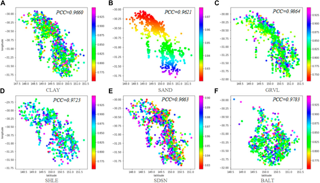
FIGURE 6. Lithology spatial distribution in the GRU_Kriging model.
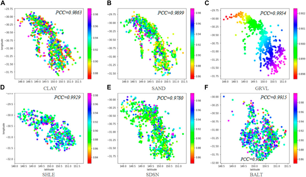
FIGURE 7. Lithology spatial distribution in the NG_GRU_Kriging model.
The proposed NG_GRU_Kriging method can fully extract the spatial features (Figure 6), and all the predicted single lithology information has a higher fitting degree (PCC>97.5%). PCC of the comprehensive lithology prediction is 98.12%, which is 5.85% and 2.01% higher than the Kriging model and GRU_Kriging model, respectively. It can better capture the spatial information between well positions and reproduce the borehole location.
3.4 Reliability analysis under the non-Gaussian hypothesis
The reliability of the DNN model is analyzed based on Bayesian theory. In terms of the Gaussian hypothesis modeling problem, the GS_INEK method is utilized to assimilate the non-Gaussian weight parameters in real-time.
Figures 5–7 track the reliability of the single lithology prediction dynamically. The color bar graph represents the reliability probability values. Table 3 details the extreme range. Compared with Kriging model, the reliability of NG_GRU_Kriging model improved by 6.50%–12.46%, 10.79%–5.39%, 15.48%–4.02%, 10.05%–2.49%, 8.69%–4.96%, and 10.47%–4.46%, respectively. Compared with GRU_Kriging model, the reliability of NG_GRU_Kriging model improved by 1.51%–7.47%, 6.33%–4.74%, 14.8%–3.72%, 14.87%–4.25%, 8.79%–12.97%, and 5.89%–10.76%, respectively.
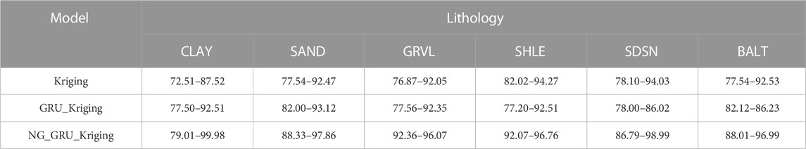
TABLE 3. Reliability range of inverted single lithology in the different models (%).
Figures 8–10 show the histograms of the model reliability of each lithology. The Kriging model has a wide range of single lithology reliability distribution. The central points are located at 0.790, 0.840, 0.8420, 0.825, 0.842, and 0.815, respectively. Although the reliability extremes of lithology SHLE, SDSN, and BALT of the GRU_Kriging method are slightly larger than those of the Kriging method, the reliability distribution range is more concentrated, with the center points located around 0.846, 0.853, 0.848, 0.852, 0.893, and 0.867, respectively. The reliability of all the results in the NG_GRU_Kriging model is over 0.900, except for CLAY lithology (0.800–0.998). The centers are located around 0.900, 0.923, 0.956, 0.913, 0.908 and 0.932, respectively.
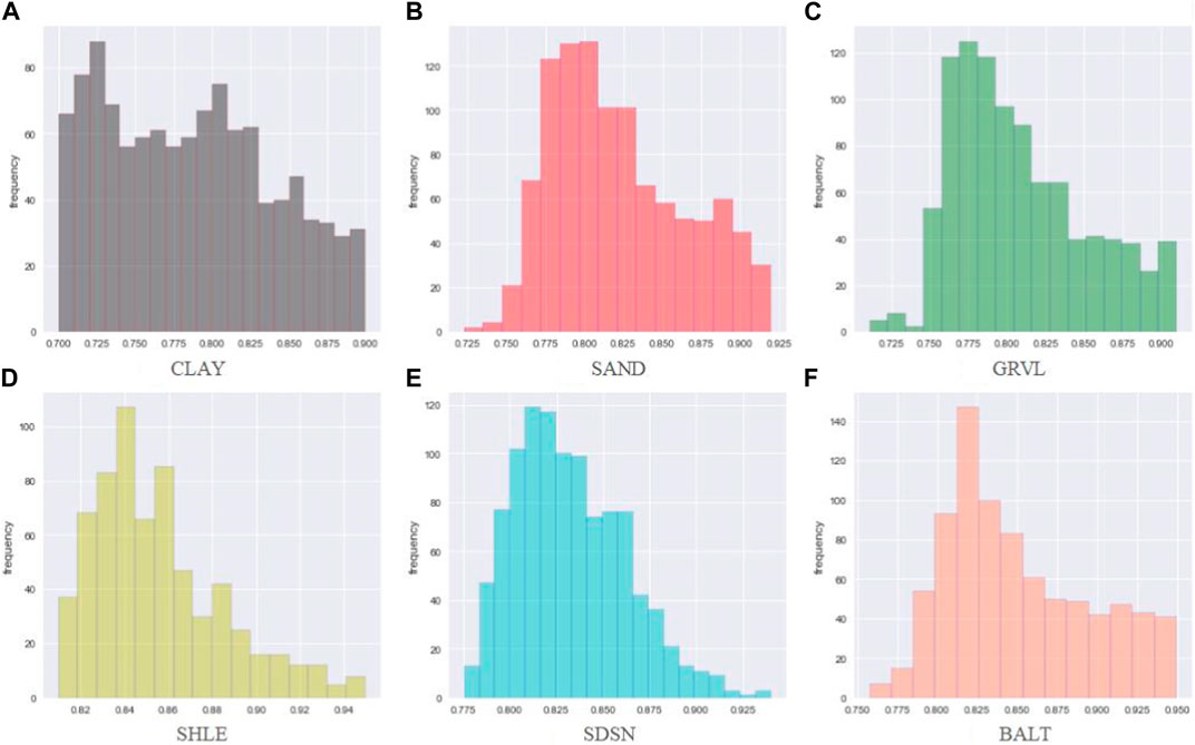
FIGURE 8. Reliability distribution of the Kriging model.
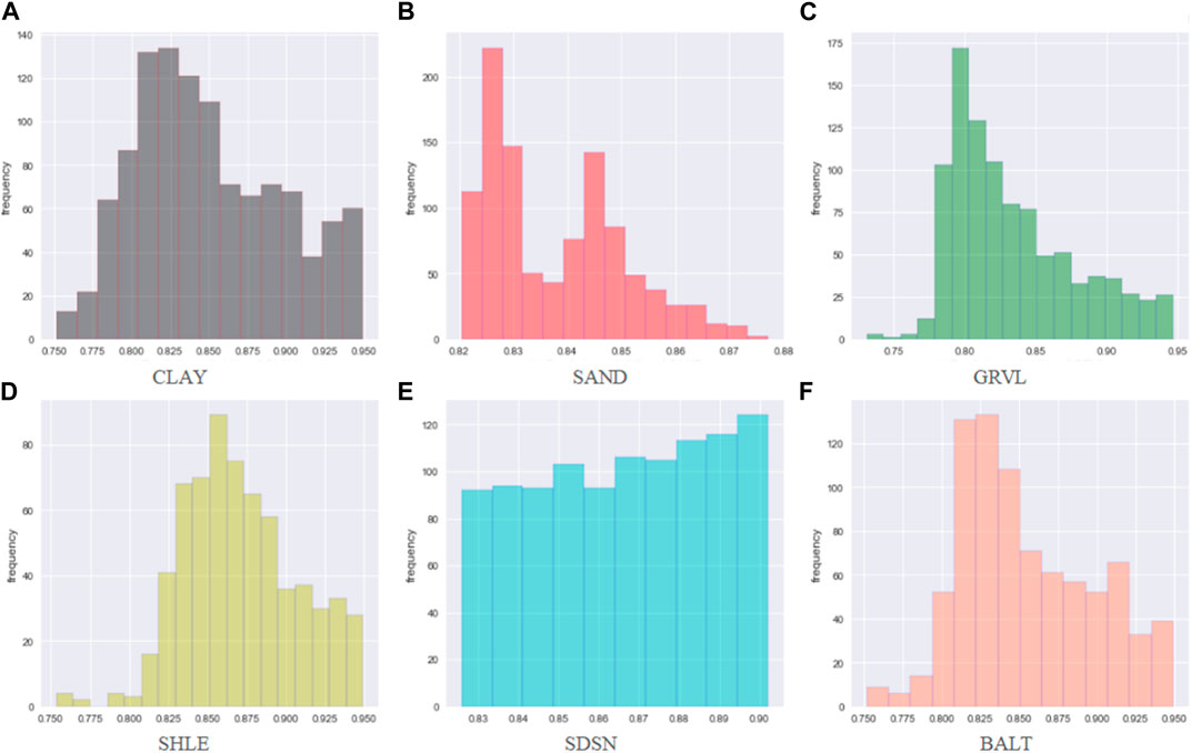
FIGURE 9. Reliability distribution of the GRU_Kriging model.
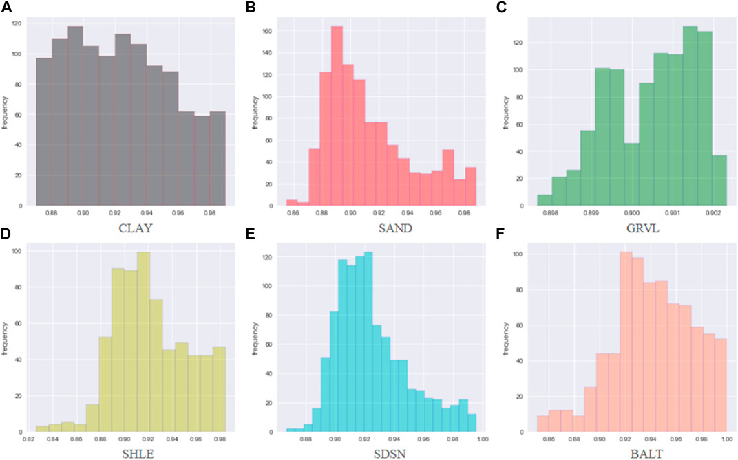
FIGURE 10. Reliability distribution of NG_GRU_Kriging model.
The distribution of the comprehensive reliability is shown in Figure 11. The distribution range of the Kriging model is wide (0.700–0.950), with a maximum value of around 0.825. There are 325 lithology data with a reliability of over 0.900, the reliability of 3,553 lithology data ranges from 0.800 to 0.900, and 1,770 lithology data with have a reliability of between 0.700 and 0.800. The reliability range of the GRU_Kriging model is 0.720–0.950, and the center point is around 0.850. There are 638 lithology data with a reliability over 0.900, the reliability of 4,549 lithology data is between 0.813 and 0.900, and 1,770 lithology data with a reliability is between 0.700 and 0.800. The reliability distribution range of the NG_GRU_Kriging model is relatively concentrated (0.880–0.960). Of particular note, the reliability of the inverted results is all over 0.880, among which 4,183 lithology data have a reliability of more than 0.900.
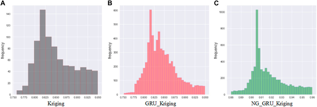
FIGURE 11. Comprehensive reliability distribution in the different models.
The method is applied to the shale reservoir in the North Sea basin, and the spatial distribution of heterogeneous reservoir lithology is predicted by using the existing spatial coordinate information, density, natural gamma ray, deep lateral resistivity, and acoustic. The fitting degree of the comprehensive lithology model is 95.072%, the average absolute percentage error is 1.5113%, and the reliability of single lithology identification results is higher than 90.61%. The experimental results indicate that the proposed method can be applied to the spatial distribution of lithology in other related fields and has a certain universality.
3.5 Training time analysis
The training time of the models is tested under the same running environment. Figure 12 shows the training time for different data samples in the Kriging, GRU_Kriging, and NG_GRU_Kriging models.
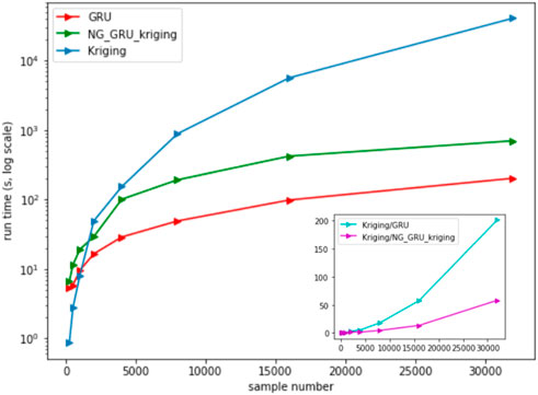
FIGURE 12. Training time in the different models.
The Kriging method has a shorter training time when the data samples are less than 1,000. As the sample size increases, the time cost of training increases exponentially. The small graph in the lower right corner of Figure 12 shows the time-multiple relationship with the other two models. GRU_Kriging model has a certain advantage in time performance. NG_GRU_Kriging method is modeled under the non-Gaussian hypothesis, and the real-time update process of non-Gaussian data requires a certain time cost. High-reliable and high-accuracy results are obtained with smaller time defects, which is beneficial to improve the universality of reservoir prediction systems based on deep learning in specific engineering problems.
4 Discussion
Combined with Kriging and deep learning technology, the NG_GRU_Kriging method can realize the prediction of heterogeneous reservoir lithology spatial distribution and model reliability evaluation according to the relevant reservoir attributes and spatial features. The method is applied to the laterite nickel ore heterogeneous reservoir, and the lateral distribution of reservoir lithology is finely depicted in both longitude and latitude directions.
The NG_GRU_Kriging method can model the spatial dependence and fully extract the key feature information from the nonlinear relationship of the reservoir data, which can accurately describe the horizontal spatial geological trend of reservoir lithology. Especially, it has good spatial tracking ability in the lateral direction of the reservoir. The method can provide basic data support and a decision-making basis for improving drilling and completion strategies.
The NG_GRU_Kriging method effectively gives the blind area of the model for different input data without assuming any data distribution. Combining the model reliability evaluation with the actual data distribution, the reliability of the prediction is higher than that of the other two models. Analyze the results with low reliability in the practical application, which improves the universality of the model in the practical engineering field.
Compared with the Kriging method, the NG_GRU_Kriging method has obvious advantages in the training speed. It reduces computational cost and has stronger scalability for large data samples. The training time of the NG_GRU_Kriging method is slightly higher than that of the GRU_Kriging method. However, it has obtained more reliable and accurate predicted results of lithology distribution. The deep learning model constructed in a non-Gaussian environment has stronger engineering applicability.
5 Conclusion
This study focuses on the problem of the Gaussian hypothesis in reservoir prediction and reliability analysis modeling. The proposed NG_GRU_Kriging method plays an important role in this research, which realizes reservoir lithology spatial distribution prediction and reliability analysis under a non-Gaussian hypothesis. It explores the distribution of lithology spatial distribution in lateral space, and further research will focus on the distribution in depth direction. The case study of heterogeneous reservoirs and experimental analysis reveals the following conclusions.
(1) The NG_GRU_Kriging method can realize intelligent prediction of heterogeneous reservoir lithology spatial distribution. It is conducive to finding future drilling positions and improving the production of oil and gas and solid energy, which can reduce the logging cost and improve the drilling and completion strategy.
(2) The SDDK technology can obtain more spatial key information with less time cost compared with deep learning and Kriging technology. The technology is scalable to massive datasets, which can reduce computational costs, and improve model accuracy and engineering applicability.
(3) The GS_IENKF method assimilates the non-Gaussian data in real time. It ensures the quantitative reliability evaluation of the prediction system under the non-Gaussian hypothesis, and can effectively reduce the economic loss or social impact caused by the unpredictability of neural networks. The model reliability analysis can achieve system risk assessment and assist it in making better decisions.
Data availability statement
The data analyzed in this study is subject to the following licenses/restrictions: The copyright of the dataset belongs to Northeast Petroleum University. Requests to access these datasets should be directed to emxsQG5lcHUuZWR1LmNu.
Author contributions
LZ proposed the spatial distribution method and constructed the model, and was the main writer of the manuscript. WR was mainly responsible for manuscript editing, model verification, and financial support. LS was responsible for the model construction and model verification. YN and XL completed the data processing work. All authors contributed to the article and approved the submitted version.
Funding
This work was supported by the Natural Science Foundation of Hebei Province of China (D2022107001), the Key of Program of the National Natural Science Foundation of China under Grants (61933007, 61873058, and 42002138).
Conflict of interest
The authors declare that the research was conducted in the absence of any commercial or financial relationships that could be construed as a potential conflict of interest.
Publisher’s note
All claims expressed in this article are solely those of the authors and do not necessarily represent those of their affiliated organizations, or those of the publisher, the editors and the reviewers. Any product that may be evaluated in this article, or claim that may be made by its manufacturer, is not guaranteed or endorsed by the publisher.
References
Airaudo, M., Nistico, S., and Zanna, L. F. (2015). Learning, monetary policy, and asset prices. J. Money Credit Bank. 47 (7), 1–1307. doi:10.5089/9781498343466.001
Borup, D. T., Johnson, S. A., Kim, W. W., and Berggren, M. J. (1992). Nonperturbative diffraction tomography via Gauss-Newton iteration applied to the scattering integral equation. Ultrason. Imaging 14 (1), 69–85. doi:10.1016/0161-7346(92)90073-5
Brand, N. W., Butt, C., and Elias, M. (1998). Nickel laterites:classification and features. Ind. Med. Surg. 17 (4), 181–183.
Cho, K., Van Merrienboer, B., Gulcehre, C., Bahdanauet, D., Bougares, F., Schwenk, H., et al. (2014). Learning phrase representations using RNN encoder-decoder for statistical machine translation. Comput. Sci. D14-1179, 172–1734. doi:10.3115/v1/D14-1179
Choi, Y., El-Khamy, M., and Lee, J. (2018). Universal deep neural network compression. Comput. Sci. 14 (4), 715–726. doi:10.1109/JSTSP.2020.2975903
Denker, J. S., and Lecun, Y. (1991). Transforming neural-net output levels to probability distributions advances in neural information processing systems (NIPS 1990).
Dennis, J. E. (1996). Numerical methods for unconstrained optimization and nonlinear equations. SIAM Classics in Applied Mathematics.
Du, D., Wang, C., Du, X., Yan, S., Ren, X., Shi, X., et al. (2020). Distance-gradient-based variogram and Kriging to evaluate cobalt-rich crust deposits on seamounts. Ore Geol. Rev. 84, 218–227. doi:10.1016/j.oregeorev.2016.12.028
Emery, X. (2008). Uncertainty modeling and spatial prediction by multi-Gaussian kriging:Accounting for an unknown mean value. Comput. Geosciences 34 (11), 1431–1442. doi:10.1016/j.cageo.2007.12.011
Erten, G. E., Yavuz, M., and Deutsch, C. V. (2022). Combination of machine learning and Kriging for spatial estimation of geological attributes. Nat. Resour. Res. 31, 191–213. doi:10.1007/s11053-021-10003-w
Gal, Y., and Ghahramani, Z. (2015). Dropout as a bayesian approximation: representing model uncertainty in deep learning. JMLR.Org. 48, 1050–1059. doi:10.48550/arXiv.1506.02142
Gerstmann, H., Doktor, D., Gläßer, C., and Möller, M. (2016). Phase: a geostatistical model for the Kriging-based spatial prediction of crop phenology using public phenological and climatological observations. Comput. Electron. Agric. 127, 726–738. doi:10.1016/j.compag.2016.07.032
Gratton, S., Lawless, A. S., and Nichols, N. K. (2007). Approximate Gauss–Newton methods for nonlinear least squares problems. Siam J. Optim. 18 (1), 106–132. doi:10.1137/050624935
Gu, Y., and Oliver, D. (2007). An iterative ensemble kalman filter for multiphase fluid flow data assimilation. SPE J. 12, 438–446. doi:10.2118/108438-pa
Guo-Shun, L., Hou-Long, J., Shu-Duan, L., Xin-Zhong, W., Hong-Zhi, S., Yong-Feng, Y., et al. (2010). Comparison of kriging interpolation precision with different soil sampling intervals for precision agriculture. Soil Sci. 175 (8), 405–415. doi:10.1097/SS.0b013e3181ee2915
Hansen, T. M., Mosegaard, K., Pedersen-Tatalovic, R., Uldall, A., and Jacobsen, N. L. (2008). Attribute-guided well-log interpolation applied to low-frequency impedance estimation. Geophysics 73 (6), 83–95. doi:10.1190/1.2996302
Hauptmann, A., Arridge, S., Lucka, F., Muthurangu, V., and Steeden, J. A. (2018). Real-time cardiovascular MR with spatio-temporal artifact suppression using deep learning - proof of concept in congenital heart disease. Comput. Sci. 81 (2), 1143–1156. doi:10.1002/mrm.27480
Heaton, M. J., Datta, A., Finley, A. O., Furrer, R., Guinness, J., Guhaniyogi, R., et al. (2018). A case study competition among methods for analyzing large spatial data. J. Agric. Biol. Environ. Statistics 12, 398–425. doi:10.1007/s13253-018-00348-w
Janssen, H. (2013). Monte-Carlo based uncertainty analysis: sampling efficiency and sampling convergence. Reliab. Eng. ? System Safety 109 (2), 123–132. doi:10.1016/j.ress.2012.08.003
Korjani, M. M., Popa, A. S., Grijalva, E., Cassidy, S. D., and Ershaghi, I. (2016). Reservoir characterization using fuzzy Kriging and deep learning neural networks, in SPE Annual Technical Conference and Exhibition.
Liu, X. T., Firoz, J., Aksoy, S., Amburg, L., Lumsdaine, A., Joslyn, C., et al. (2022). High-order line graphs of non-uniform hypergraphs: algorithms, applications, and experimental analysis, in 2022 IEEE International Parallel and Distributed Processing Symposium (IPDPS), 784–794. doi:10.1109/IPDPS53621.2022.00081
MacKay, D. J. C. (1992). A practical bayesian framework for backpropagation networks. Neural Computation 4 (3), 448–472. doi:10.1162/neco.1992.4.3.448
Moehrle, M. G. (2019). Similarity measurement in times of topic modelling. World Patent Information 59, 101934. doi:10.1016/j.wpi.2019.101934
Montavon, G., Lapuschkin, S., Binder, A., Samek, W., and Müller, K. R. (2016). Explaining NonLinear classification decisions with deep taylor decomposition. Pattern Recognition 65, 211–222. doi:10.1016/j.patcog.2016.11.008
Natekar, P., Kori, A., and Krishnamurthi, G. (2020). Demystifying brain tumor segmentation networks: interpretability and uncertainty analysis. Frontiers in Computational Neuroscience 14, 6. doi:10.3389/fncom.2020.00006
Ning, Q., Dong, W., Shi, G., Li, L., and Li, X. (2021). Accurate and lightweight image super-resolution with model-guided deep unfolding network. IEEE Journal of Selected Topics in Signal Processing 15 (2), 240–252. doi:10.1109/JSTSP.2020.3037516
Nowak, W., and Litvinenko, A. (2013). Kriging and spatial design accelerated by orders of magnitude: combining low-rank covariance approximations with FFT-techniques. Mathematical Geosciences 45, 411–435. doi:10.1007/s11004-013-9453-6
Odeh, I., Todd, A. J., and Triantafilis, J. (2003a). Spatial prediction of soil particle-size fractions as compositional data. Soil Science 168 (7), 501–515. doi:10.1097/01.ss.0000080335.10341.23
Odeh, I., Todd, A. J., and Triantafilis, J. (2003b). Spatial prediction of soil particle-size fractions as compositional data. Soil Science 168 (7), 501–515. doi:10.1097/01.ss.0000080335.10341.23
Odeh, I. O. A., Todd, A. J., and Triantafilis, J. (1997). Approximating a cumulative distribution function by generalized hyperexponential distributions. Probability in the Engineering and Informational Sciences 11 (01), 11–18. doi:10.1017/S0269964800004630
Ogawa, H., and Oja, E. (1986). Projection filter, Wiener filter, and Karhunen-Loève subspaces in digital image restoration. Journal of Mathematical Analysis and Applications 114 (1), 37–51. doi:10.1016/0022-247X(86)90063-6
Pak, U., Ma, J., Ryu, U., Ryom, K., Juhyok, U., Pak, K., et al. (2020). Deep learning-based PM2.5 prediction considering the spatiotemporal correlations: a case study of Beijing, China. The Science of the Total Environment 616-617 (10), 133561.1–133561.11. doi:10.1016/j.scitotenv.2019.07.367
Pearl, J. (1990). Probabilistic reasoning in intelligent systems: networks of plausible inference. Artificial Intelligence 48 (8), 117–124. doi:10.2307/2026705
Robert, J. W., Jacqueline, A., Lloyd, D. G., and Ajmal, M. (2018) Predicting athlete ground reaction forces and moments from spatio-temporal driven CNN models. IEEE Transactions on Biomedical Engineering 66(3):689–694. doi:10.1109/TBME.2018.2854632
Salakhutdinov, R., and Hinton, G. (2012). An efficient learning procedure for deep Boltzmann machines. Neural Computation 24 (8), 1967–2006. doi:10.1162/NECO_a_00311
Schaback, R. (1995). Error estimates and condition numbers for radial basis function interpolation. Advances in Computational Mathematics 3 (3), 251–264. doi:10.1007/BF02432002
Suresha, M., Kuppa, S., and Raghukumar, D. S. (2020). A study on deep learning spatiotemporal models and feature extraction techniques for video understanding. International Journal of Multimedia Information Retrieval 9 (2), 81–101. doi:10.1007/s13735-019-00190-x
Walvoort, D., and Gruijter, J. (2001). Compositional Kriging: a spatial interpolation method for compositional data. Mathematical Geology 33 (8), 951–966. doi:10.1023/a:1012250107121
Xu, M., Liu, J., Du, J., Gu, S., and Liang, S. (2013). Progress in prospecting of gold and copper polymetallic deposits in the New England orogenic belt, New South Wales, Australia. Mineral Exploration 4 (6), 707–713. doi:10.3969/j.issn.1674-7801.2013.06.017
Zeng, L., Ren, W., Shan, L., and Huo, F. (2021). Well logging prediction and uncertainty analysis based on recurrent neural network with attention mechanism and Bayesian theory. Journal of Petroleum Science and Engineering 208 (B), 109458. doi:10.1016/j.petrol.2021.109458
Zhang, Y., Lu, M., and Li, H. (2020). Urban traffic flow forecast based on FastGCRNN. Journal of Advanced Transportation 2020 (12), 1–9. doi:10.1155/2020/8859538
Zhou, H., Gomez-Hernandez, J. J., Franssen, H., and Li, L. (2011). An approach to handling non-Gaussianity of parameters and state variables in ensemble Kalman filtering. Advances in Water Resources 34 (7), 844–864. doi:10.1016/j.advwatres.2011.04.014
Zimmerman, D. L., and Holland, D. M. (2005). Complementary co-kriging:spatial prediction using data combined from several environmental monitoring networks. Environmetrics 16 (3), 219–234. doi:10.1002/env.699
Keywords: lithology spatial distribution, kriging technology, non-Gaussian hypothesis, deep learning, reliability analysis
Citation: Zeng L, Ren W, Shan L, Niu Y and Liu X (2023) Prediction and reliability analysis of reservoir lithology spatial distribution. Front. Earth Sci. 11:1251218. doi: 10.3389/feart.2023.1251218
Received: 01 July 2023; Accepted: 26 October 2023;
Published: 27 December 2023.
Edited by:
Zhihao Xu, Guangdong University of Technology, ChinaCopyright © 2023 Zeng, Ren, Shan, Niu and Liu. This is an open-access article distributed under the terms of the Creative Commons Attribution License (CC BY). The use, distribution or reproduction in other forums is permitted, provided the original author(s) and the copyright owner(s) are credited and that the original publication in this journal is cited, in accordance with accepted academic practice. No use, distribution or reproduction is permitted which does not comply with these terms.
*Correspondence: Weijian Ren, cmVud2pAMTI2LmNvbQ==