Assessing turbulence and mixing parameterizations in the gray-zone of multiscale simulations over mountainous terrain during the METEX21 field experiment

Multiscale numerical weather prediction models transition from mesoscale, where turbulence is fully parameterized, to microscale, where the majority of highly energetic scales of turbulence are resolved. The turbulence gray-zone is situated between these two regimes and multiscale models must downscale through these resolutions. Here, we compare three multiscale simulations which vary by the parameterization used for turbulence and mixing within the gray-zone. The three parameterizations analyzed are the Mellor-Yamada Nakanishi and Niino (MYNN) Level 2.5 planetary boundary layer scheme, the TKE-1.5 large eddy simulation (LES) closure scheme, and a recently developed three-dimensional planetary boundary layer scheme based on the Mellor-Yamada model. The simulation domain includes complex (i.e., mountainous) terrain in Nevada that was instrumented with meteorological towers, profiling and scanning lidars, a tethered balloon, and a surface flux tower. Simulations are compared to each other and to observations, with assessment of model skill at predicting wind speed, wind direction and TKE, and qualitative evaluations of transport and dispersion of smoke from controlled releases. This analysis demonstrates that microscale predictions of transport and dispersion can be significantly influenced by the choice of turbulence and mixing parameterization in the terra incognita, particularly over regions of complex terrain and with strong local forcing. This influence may not be apparent in the analysis of model skill, and motivates future field campaigns involving controlled tracer releases and corresponding modeling studies of the turbulence gray-zone.

1 Introduction and motivation

With advances in computing resources, multiscale atmospheric simulations that resolve scales of motion ranging between the mesoscale (Δ ≳ 1 km) and microscale (Δ ≲ 100 m), which includes the so-called turbulence “gray-zone,” are becoming increasingly mainstream. Recent studies have demonstrated that by resolving and downscaling large-scale flow features and turbulence, a multiscale approach can improve predictions of transport and dispersion compared to a microscale-only approach (Wiersema et al., 2020; Wiersema et al., 2022; Nagel et al., 2022). Here, we analyze and compare multiscale simulations of the Meteorology Experiment 2021 (METEX21) field campaign with the objective of developing insight into the choice of turbulence parameterization for domains within the turbulence gray-zone and providing a set of case study days to assist the modeling community with developing recommendations and “best practices” for future multiscale modeling endeavors.

In multiscale simulations, inaccuracy on a parent domain will impact the solution of any child domains. By definition, a multiscale nested simulation includes at least two regimes, a mesoscale domain where the majority of energetic turbulence is subgrid-scale and a microscale domain where the majority of energetic turbulence is resolved. Because of the disconnect between the mesoscale and microscale, multiscale simulations typically include at least one intermediate domain within the turbulence gray-zone. Also referred to as the terra incognita, the gray-zone is a numerical regime where the dominant energy-containing length scales of turbulence are roughly the same scale as the grid resolution (Wyngaard, 2004). In this regime, one-dimensional planetary boundary layer (PBL) schemes are inappropriate because large turbulent features are resolved, however large eddy simulation (LES) turbulence closure models are also unsuitable because the majority of energetic turbulence is unresolved. Additionally, horizontal gradients are often non-negligible within the gray-zone, which invalidates the assumption of horizontal homogeneity made by PBL schemes. While the numerical weather prediction community has extensively developed and compared PBL schemes for mesoscale simulations (Hu et al., 2010; Peña and Hahmann, 2020), and the engineering community has reviewed LES techniques for microscale simulations (Meneveau and Katz, 2000), there is not yet consensus on “best practices” for configuring intermediate domains within the terra incognita for multiscale simulations.

The terra incognita is receiving increasing attention from the atmospheric modeling community, including several noteworthy reviews and modeling studies. Chow et al. (2019), Honnert et al. (2020), and Dudhia (2022) provide clear and thorough descriptions of the challenges associated with modeling at gray-zone resolutions. Efstathiou and Beare (2015) investigated the partitioning of resolved and subgrid diffusion at gray-zone resolutions and emphasizes the complexity of modeling in this regime. These studies have focused on model fidelity at gray-zone resolutions, but multiscale modelers are typically most interested in microscale domains that are intrinsically connected to their gray-zone parent domains. It is important to understand the relevance of domains with gray-zone resolutions in the context of a multiscale simulation. Specifically, how, when, and to what extent domains with gray-zone resolution influence nested microscale domains.

Here, we evaluate multiscale simulations of transport and mixing over complex (i.e., mountainous) terrain with four primary motivations. First, to investigate transport and dispersion during METEX21 and examine how the choice of turbulence and mixing parameterization in the gray-zone effects microscale predictions. Second, to evaluate performance of the three-dimensional planetary boundary layer (3D PBL) scheme of Kosović et al. (2020) and Juliano et al. (2022), detailed in Section 4. Third, to provide the multiscale modeling community with a case-study, including lessons learned regarding the model configuration and performance. It is important to note that numerous and diverse case studies are necessary for the modeling community to establish “best practices” regarding multiscale modeling. And fourth, to motivate future model development by examining model limitations and uncertainties.

For this study, we compare three methods used to parameterize turbulence and mixing in the turbulence gray-zone; a PBL scheme, a LES closure model, and the 3D PBL scheme. Effort has been taken to reduce simulation complexity by minimizing the number of nested domains, which simplifies the analysis and emphasizes the differences between the simulations. The simulations use a three-domain nested configuration, shown in Figure 1 and described in detail in Section 3, with the outermost domain at mesoscale resolution (Δ_x = 2,520 m), the intermediate domain (Δ_x = 280 m) at a resolution within the terra incognita, and the innermost domain at microscale resolution (Δ_x = 40 m). The calculation and discussion of model skill for prediction of wind speed, wind direction, and turbulence kinetic energy is presented in Section 5. Section 6 includes qualitative analysis of transport and dispersion and comparisons to scanning lidar observations.

FIGURE 1

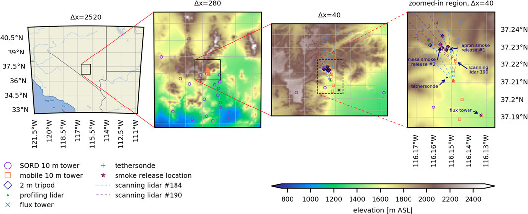
FIGURE 1. Grid layout of the three nested domains, including filled terrain contours and selected METEX21 sensor locations on D2 and D3. The fourth panel shows a zoomed-in section of D3 that more clearly displays the dense network of instruments located near the P-tunnel apron. Dashed lines are used to indicate the orientation of the scanning lidar RHI sweeps. Annotations of the sweep numbers for scanning lidar #190 are included in the zoomed-in panel.

2 Meteorology experiment 2021 case study

METEX21 was a field campaign designed to observe meteorology and transport and dispersion in the PBL over complex mountainous terrain. Observations for METEX21 were collected March 20–28 2021 at the Nevada National Security Site (NNSS) with an emphasis on a 5 km by 5 km region of desert flats, rugged canyons, and mesas in NNSS Area 12. Centered within this 25 km² domain is a hillside tunnel entrance, henceforth referred to as the P-tunnel. The hillside has a flat region near the base of the mesa and in front of the P-tunnel entrance that is referred to as the P-tunnel apron, which is a location of interest during METEX21. Vegetation within the experiment domain varied from juniper and Piñon pine woodland on the mesa tops to blackbrush and sagebrush at lower elevations. Photographs of the site and detailed descriptions of the field campaign planning, sensor deployment, and data collection are available in an accompanying paper to this Special Issue by Wharton et al.

Here, we simulate three case periods of interest with each beginning at 1200 UTC (5 a.m. local time) and ending at 0000 UTC (5 p.m. local time) on March 21st, 22nd and 28th of 2021. Multiple controlled releases of smoke occurred on each of these days and are described in more detail below. Conditions throughout March 21st included dominant synoptic forcing and uniform northwesterly winds. On the 22nd, conditions were locally forced and a wind direction shift was observed in the flats and canyons below the mesa while consistent northwesterly winds were found aloft and on the mesa tops. Winds on the 28th started off north-northwesterly and transitioned to southeasterly at all sites as the day progressed. Cloud cover and precipitation were negligible during all of the time periods evaluated.

During METEX21, the complex flow near the P-tunnel apron was directly observed through the controlled release of smoke from seven release locations. Three locations along the top of the mesa edge, one location midway up the mesa slope, and three locations along the P-tunnel apron were selected in combinations to form release scenarios including a “horizontal transect” roughly along the elevation contour of the P-tunnel apron, a “vertical transect” along the slope between the P-tunnel apron and the mesa edge, and a set of locations along the mesa cliff referred to as “mesa edge.” The highest and lowest release locations in the vertical transect scenario had an elevation difference of 250 m. Each release consisted of approximately 20 smoke candles set at ground level and ignited in batches to create a nearly continuous 30 min smoke plume. Releases were observed in-person and by a series of video cameras. Additionally, two portable optical particle counter (POPS) were deployed at approximately 80 and 300 m AGL on the tethersonde at a distance of 2 km from the smoke release locations. However, the plumes were not clearly detected by the POPS. This may be due to the distance from the release location and very low concentrations at these distances.

The scanning lidars proved more successful at tracking the smoke plumes nearby (i.e., within a kilometer of) the release locations and these results are compared to the atmospheric simulations in more detail below. Figure 1 shows topography near the P-tunnel apron with markers indicating locations of smoke release locations and observational sensors, including orientations of scanning lidar RHI (range-height-indicator) sweeps directed towards the P-tunnel. Sweep #3 by scanning lidar #190, which is at an elevation of 1,615 m ASL, roughly follows the vertical transect release scenario including the Apron-1, Mesa-4, and Mesa-2 release locations, which have elevations of 1,660, 1,741, and 1,903 m ASL, respectively.

Simulations are evaluated using a combination of quantitative and qualitative comparisons between each other and versus observations collected during the METEX21 field campaign. Observations used in this analysis include two scanning lidar systems, three profiling lidar systems, 31 10 m meteorological towers, 6 3-d sonic anemometers mounted on 2 m tripods, one 3 m flux tower, one tethered balloon system, and multiple balloon-launched radiosondes.

3 Model configurations

Simulations are run with the Weather Research and Forecasting (WRF) model version 4.0.3 (Skamarock et al., 2021). The three nested domains will henceforth be referred to as D1 (mesoscale Δ_x = 2,520 m), D2 (intermediate Δ_x = 280 m), and D3 (microscale Δ_x = 40 m). Additional details regarding the model configuration are included in Table 1. Turbulence and mixing are parameterized by the Mellor-Yamada Nakanishi and Niino (MYNN) level-2.5 PBL scheme (Nakanishi and Niino, 2006) on D1, and the turbulent kinetic energy 1.5 order (TKE1.5) subgrid-scale (SGS) model (Deardorff, 1980) on D3. The three configurations compared in this study vary by the turbulence and mixing parameterization used on D2, which is MYNN, TKE1.5, or the 3D PBL scheme of Kosović et al. (2020) and Juliano et al. (2022) that is detailed in Section 4.

TABLE 1

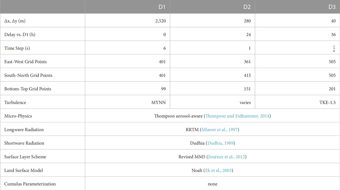
TABLE 1. Summary of the model configuration including grid sizes and physics parameterizations. MYNN is Mellor-Yamada Nakanishi and Niino Level 2.5 PBL scheme. TKE-1.5 is the 1.5 order TKE LES closure scheme.

D1 is initialized and forced with output from the High Resolution Rapid Refresh (HRRR) model (Benjamin et al., 2016). Topography for D2 and D3 is sampled from the Shuttle Radar Topography Mission dataset, which has approximately 1 arcsecond resolution (Farr et al., 2007). Land characteristics data is sampled from the National Land Cover Database, which has approximately 9 arcsecond resolution. Shading of incoming solar radiation by topography is enabled, which calculates complex terrain shadows near sunrise and sunset. These high-resolution datasets and model configuration options are essential for capturing the local-scale temperature and pressure differences that drive upslope and downslope flows in the mountain-valley terrain.

Control over the grid aspect ratio and vertical resolution of each domain is necessary because the vertical grid of the mesoscale domain D1 is inappropriate for use on the microscale domain D3, and vice versa. The vertical grid refinement method of Daniels et al. (2016) allows each domain to have a unique number and placement of vertical grid levels. D1 has 99 vertical levels with placement determined by the default WRF model algorithm. D2 has 151 vertical levels with near-surface spacing of 17.5 m until 315 m AGL after which levels are progressively stretched by ∼4.4% until 1,500 m AGL. The remaining levels are progressively stretched by ∼1.4% until reaching the model top. D3 has 201 vertical levels with near-surface spacing of 10 m until 150 m AGL after which levels are progressively stretched by ∼4.5% until 1,000 m AGL. The remaining levels are progressively stretched by ∼0.9% until reaching the model top. The model top for all domains is at 10,000 Pa.

The cell perturbation method (CPM) of Muñoz-Esparza et al. (2014), Muñoz-Esparza et al. (2015), and Muñoz-Esparza and Kosović (2018) is applied along the lateral boundaries of the most coarse LES domain of each simulation. The CPM accelerates the development of small-scale turbulence following transition through a grid refinement interface by introducing small perturbations to the potential temperature field. Here, the CPM is enabled when transitioning from a PBL or 3DPBL domain to an LES domain. For simulations where D2 is run with the PBL or 3DPBL scheme, the perturbations are added to D3. For simulations where D2 is run with the LES SGS model, the perturbations are added to D2.

A passive tracer gas is released in D3 to mimic the smoke releases during METEX21. Because of uncertainty regarding the exact source strength of the smoke candles, each release location has a modeled source strength of 1 g·s⁻¹ and the following analysis focuses on comparisons of plume shape. Feedback from child to parent domains is disabled (i.e., one-way nesting is used). However, an exception is made for the passive tracer, which is upscaled from D3 to D2 and from D2 to D1. Note that nest feedback is not possible in the standard WRF code when vertical grid refinement is used. A new option for tracer-only feedback with vertical grid refinement was added to the code as part of this work.

4 3D PBL parameterization

The three-dimensional planetary boundary layer (3D PBL) scheme, recently developed in WRF for atmospheric simulations in the gray zone by Kosović et al. (2020) and Juliano et al. (2022), is tested here in the complex environment of METEX21. The scheme, based on Mellor and Yamada (1974) and Mellor and Yamada (1982), calculates both horizontal and vertical turbulent fluxes for use in the model equations for momentum, potential temperature, and moisture. Its treatment of the horizontal fluxes distinguishes the 3DPBL scheme from MYNN and other common one-dimensional schemes, which calculate vertical fluxes only and rely on a two-dimensional version of the Smagorinsky model to parameterize horizontal fluxes (Smagorinsky, 1963). In practice, the horizontal Smagorinsky treatment is often used to smooth horizontal variability, thus increasing numerical stability (Smagorinsky, 1993).

The 3DPBL scheme provides a useful comparison to MYNN because both are based on the Mellor-Yamada framework. In particular, they both parameterize turbulent fluxes by solving a prognostic equation for the TKE [see Eq. 9 in Juliano et al. (2022)]. They also depend on a diagnostic master length scale and closure constants that relate the master length scale to other length scales used in the model. These parameters differ between the two schemes, as discussed in Arthur et al. (2022). Within the 3D PBL scheme, the boundary layer approximation of Mellor and Yamada (1974) and Mellor and Yamada (1982) can be invoked to reduce computational cost and increase numerical stability. This option neglects horizontal derivatives within the algebraic system and in the prognostic TKE equation, while still allowing the 3D turbulent fluxes to be calculated analytically [see Eq. 22 in Juliano et al. (2022)].

The 3D PBL setup used here follows that of Arthur et al. (2022), which tested model performance in the complex terrain of the Columbia River Basin. Therein, the boundary layer approximation was used along with the standard formulation for the length scale and closure constants (Mellor and Yamada, 1982). Readers are referred to Juliano et al. (2022) and Arthur et al. (2022) for additional discussion of these model options. Note that here, as in Arthur et al. (2022), the full 3D PBL scheme (without the boundary layer approximation) was attempted but found to be numerically unstable. This is likely related to the limited applicability of available length scale formulations in complex terrain, which is a topic of ongoing work.

5 Model skill

Model skill tests allow for an analysis of the accuracy of model prediction relative to METEX21 observations of wind speed, wind direction, and turbulence kinetic energy. Here we evaluate the accuracy of wind speed predictions with the skill metrics HR2.0, the hit rate within 2.0 m·s⁻¹ (Eq. 1a), and FB, the fractional bias (Eq. 1b). Note that a negative (positive) FB score indicates an overprediction (underprediction). Wind direction predictions are evaluated with a metric proposed by Calhoun et al. (2004), the scaled average angle (SAA) (Eq. 1c), which more heavily weights errors in wind direction that occur at locations with high wind speed. Note that a lower SAA score corresponds to less error in the wind direction predictions. TKE predictions are evaluated with FAC2, the fraction of predictions within a factor of two of the observations (Eq. 1d), and FB.

$\text{HRx}=\text{\hspace{0.17em}fraction satisfying}{X}_o-\text{x}\le X_p\le X_o+\text{x}(\mathrm{1a})$

$\text{FB}=2\left(\overline{X_o}-\overline{X_p}\right)/\left(\overline{X_o}+\overline{X_p}\right)(\mathrm{1b})$

$\text{SAA}=\mathrm{\Sigma }\left(|U_i||{\varphi }_i|\right)/\left(N|\overline{U_i}|\right)(\mathrm{1c})$

$\text{FACx}=\text{\hspace{0.17em}fraction satisfying}1/\text{x}\le X_p/X_o\le \text{x}(\mathrm{1d})$

In Equations 1, X_o and X_p are the sets of observations and corresponding predictions, N is the number of observations, ϕ_i is the difference between observed and predicted wind directions, and |U_i| is the predicted wind speed. An overbar indicates averaging over all locations of observations. Values for X_o and X_p are time-averages over a 30 min window.

Figure 2 summarizes the model skill scores for predictions of wind speed, wind direction, and TKE at 10 m towers and 2 m tripods, and includes timeseries and mean skill scores during the three case study days analyzed. Model skill at predicting wind speed and wind direction is calculated using simulation results from D2 because all 31 of the 10 m towers are sited within D2 while only 13 are within D3. When evaluated on D3, these model skill scores show similar trends but with more noise in the timeseries due to the lower number of observation sites located within D3. Model skill at predicting resolved TKE is calculated using results from D3 because all of the observations with high-frequency output (mobile 10 m towers and 2 m tripods) are sited within D3 and we are most interested in evaluating differences within the microscale domain of the three configurations. Note that while all of the 10 m meteorological towers were equipped with 3 dimensional sonic anemometers, only ten of those (all located within D3) archived the high frequency data needed to calculate TKE.

FIGURE 2

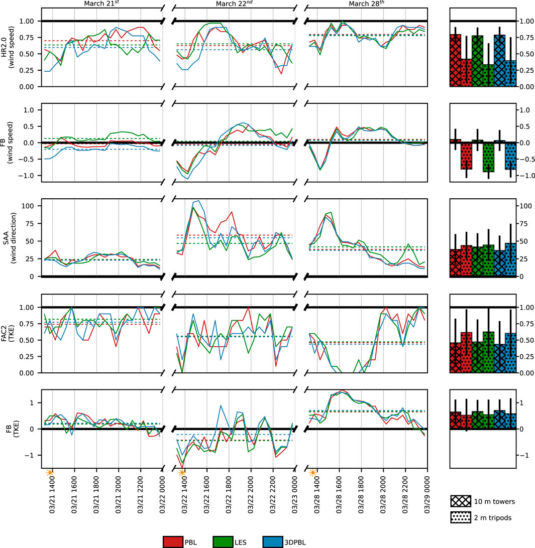
FIGURE 2. Timeseries of model skill scores and bar graphs of mean scores across the three timeperiods simulated. Observations of wind speed and wind direction are compared to predictions from D2 while observations of TKE are compared to predictions from D3. Timeseries of model skill includes only data from the 10 m towers. Bar graphs of mean scores include results reported independently for 10 m towers and 2 m tripods. Dashed horizontal lines in the timeseries correspond to mean scores during each case study day. Solid black horizontal lines correspond to the skill score of a perfect model. Estimated local sunrise times are marked with a small sun symbol along the x-axis.

With a few exceptions, differences between the skill scores of the three configurations in Figure 2 are small. The experiment-averaged skill scores display negligible differences between the PBL, 3DPBL and LES configurations. Generally, the model skill for predicting conditions at the 2 m tripods is lower than at 10 m towers, likely due to the towers being sited in unobstructed areas and higher above ground level, relative to the tripods. Skill scores for TKE are an exception due to a less severe underestimate at the tripods than at the towers. Additionally, these simulations could benefit from higher vertical resolution near the surface, which would likely improve predictions at 2 m AGL. Further refining the vertical grid would bring about additional challenges, including numerical stability limitations arising from the terrain-following vertical coordinate, increasing computational costs, and a non-optimal near-surface grid-aspect-ratio (Mirocha et al., 2010).

The timeseries of model skill include some interesting trends. Compared to March 22nd and 28th, the model skill on the 21st is nearly constant throughout the day, likely because of the consistent synoptic forcing. Wind speeds are slightly underpredicted in the LES simulation and slightly overpredicted in the 3DPBL simulation. The PBL simulation best predicts wind speed. The three simulations show comparable skill predicting wind direction and TKE. This day had the lowest overall error in predicting wind direction (northerly winds).

On March 22nd, where conditions within the valley were locally forced for most of the day, the simulations all overpredict wind speeds in the morning and underpredict wind speeds in the afternoon. The LES simulation best predicts wind directions, which is not surprising because the LES simulation is expected to best represent horizontal fluxes arising due to the thermally-driven flow over complex topography upwind on D2. All of the simulations generally overpredict TKE, with the 3DPBL simulation being the least overpredictive, but there are some brief hour-long periods of underprediction in the late morning and afternoon. The simulations show the lowest model skill in the early morning around 1500 UTC (8 a.m. local time) with large errors in wind direction and an overprediction of both wind speed and TKE. This period coincides with the atmosphere transitioning from stable to unstable as the sun rises and surface heating increases. The largest of these errors, which are shared by all of the simulations, may arise due to local-scale inaccuracy of the HRRR model, which is used for initialization and forcing of D1.

March 28th is another challenging day to simulate because of the morning transition from north-northwesterly winds to southeasterly winds. Unlike the morning transition on March 22nd, the shift in wind direction occurs nearly simultaneously at all stations and elevations throughout the 25 km² region of interest. Of the 3 days simulated, here the model skill is most similar between simulations. Model skill deteriorates in the early morning around 1500 UTC (8 a.m. local time) and recovers throughout the day. By 0000 UTC (5 p.m. local), the model skill is near perfect for all five metrics evaluated. While wind speeds are generally well predicted, the simulations underpredict TKE, which may be an indication that topography and heterogeneity of land characteristics are inadequately represented in the model and that future studies may benefit from the use of a more advanced subgrid-scale turbulence closure model and a canopy model.

Overall, the model skill shows some expected trends and a few noteworthy differences between the PBL, LES, and 3DPBL simulations. Prediction accuracy is worst in the early morning when the atmospheric stability is transitioning from stable to unstable, and best in the late afternoon when conditions are unstable and more consistent. Model skill is higher when forcing is synoptic rather than local. And the 2 m tripods are generally less predictable than the 10 m towers, which could be due to rocky terrain and nearby vegetation, such as juniper shrubs close to the tripods along the mesa edge.

Analysis of the predicted surface heat flux provides insight into a potential cause of model inaccuracy when conditions are locally-forced. Figure 3 shows the magnitude of the predicted daytime net radiation flux is generally overestimated. The overestimation in the predicted net radiation results in slightly overpredicted mid-day sensible heat fluxes as well, especially on March 22nd. The model predicts the ground heat flux and latent energy flux with high accuracy. Overall, net radiation is partitioned correctly in the model with the majority of the energy going into the sensible heat flux, followed by the ground heat flux, and very little being used for evapotranspiration (i.e., latent energy flux). Given the low soil moisture values and limited biomass in the desert valley, the energy partitioning results in a very high observed, and modeled, Bowen ratio (ratio between the sensible heat flux and latent energy flux). The accuracy in the energy partitioning in the model instills confidence that the simulations are correctly simulating daytime surface fluxes that are key to accurately prediction of near-surface flows and atmospheric mixing over complex terrain.

FIGURE 3

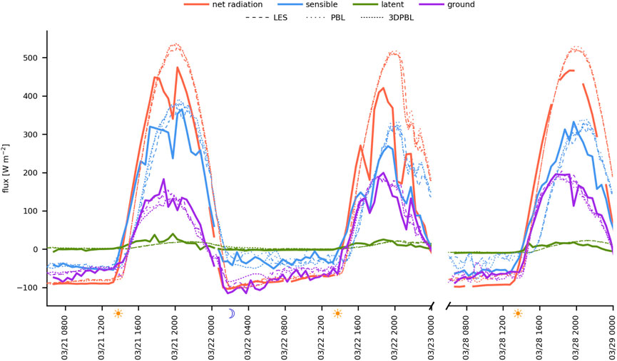
FIGURE 3. Surface energy balance observed at the Blackbrush flux tower. Observations of the 30 min averaged surface fluxes are displayed using solid lines. The 30 min rolling mean of predicted fluxes from D2 of the three simulations are shown using dashed and dotted lines. Sunrise and sunset times are indicated along the x-axis with sun and crescent moon symbols, respectively.

6 Qualitative analysis of transport and dispersion

While few substantial differences are found in the analysis of model skill at predicting wind speed, wind direction, and TKE, some noteworthy differences between the PBL, LES, and 3DPBL simulations are apparent when examining transport and dispersion of the predicted smoke plumes. Figures 4, 6, 9 show vertically integrated and time-averaged plumes from the three simulations for 1 h beginning after the start of each 30-min smoke release period. Note that results in this section focus on predictions from D3, which is always configured with an LES SGS model, but the three simulations have labels “PBL,” “3DPBL,” and “LES” according to the turbulence and mixing parameterization applied on D2. Three types of release scenarios were executed during METEX21. A series of simultaneous horizontal and vertical release transects were done on March 21st, releases along the mesa edge were done on March 22nd, and alternating horizontal and vertical transect releases were conducted on March 28th. Additional details regarding the release strategies can be found in an accompanying paper to this Special Issue. A passive tracer is released in the simulations at multiple locations matching the release strategies and sequencing of the controlled smoke releases during METEX21.

FIGURE 4

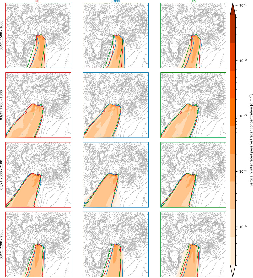
FIGURE 4. PBL, LES, and 3DPBL simulation results from D3 on March 21st with filled contours of vertically integrated passive tracer concentration. Results are time-averaged over 1-h beginning at the start times of smoke releases. To assist with visually comparing the plumes, each subplot includes colored contour lines at 10⁻⁵ g·m⁻² from the three simulations with a red contour line from the PBL simulation, blue from the 3DPBL simulation, and green from the LES simulation. Gray contour lines represent topography with spacing of 50 m. A small purple star-shaped marker indicates the location of the P-tunnel apron. The results from D3, which is always configured with an LES SGS model, are shown, but the figure labels are according to the turbulence and mixing parameterization on the parent domain, D2.

6.1 March 21st

Four smoke releases were performed on March 21st at 1500, 1700, 2000, and 2200 UTC. These were simultaneous vertical and horizontal transect release scenarios with five release locations. For these four releases, the PBL and 3DPBL simulations produce plumes of similar shape with only minor differences visible in Figure 4. During the releases beginning at 1500 and 2200 UTC, the smoke plumes predicted by the LES simulation appear more strongly affected by the complex topography, particularly to the southwest of the release location, which might be a result of differences in the large-scale turbulence and flow features that are resolved upwind on D2 and downscaled onto D3. These hours correspond to 0800 and 1500 local time. Note that local sunrise and sunset were at 0646 and 1857 local time, respectively.

Scanning lidar #190 was sited 1 km south of the P-tunnel apron and was programmed for alternating plan-position-indicator (PPI) and range-height-indicator (RHI) scan patterns while facing the P-tunnel apron. Figure 5 shows time-averaged observations and predictions between 2000 and 2100 UTC (1300–1400 local time) along RHI sweep #4 (azimuth of 335.5°) recorded by scanning lidar #190. The lidar location and the sweep orientations are shown in Figure 1. Note that in Figures 5A, B the observations recorded beneath the terrain are nonphysical and appear as regions with high levels of noise or are demarcated by prominent spikes in the attenuated backscatter. Both the observations and predictions of radial velocity indicate flow towards the lidar (flow from the north) with the maximum velocity at mesa-level overhead of the slope and a sheltered region of lower velocity flow found below mesa-level in the lee of the slope.

FIGURE 5

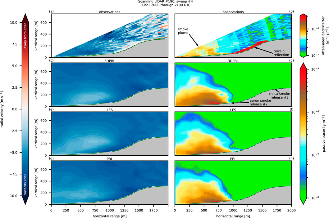
FIGURE 5. Observations of radial velocity (A) and attenuated backscatter (B) observed along sweep #4 by scanning lidar #190. Predictions from D3 of the 3DPBL, LES, and PBL simulations of radial velocity (C, E, G) and passive tracer concentration (D, F, H) along a transect defined by the scanning lidar sweep. Observations and predictions are averaged between 2000 and 2100 UTC on March 21st. Note that the observations in (A,B) include nonphysical data in regions with obscured line of sight to the scanning lidar, indicated using dashed green lines. The surface of the mesa slope is distinguished by pronounced (i.e., bright red) attenuated backscatter in (B).

Due to low concentrations of background aerosols in the desert environment, the smoke plumes are often distinguishable in the scanning lidar attenuated backscatter field. It is important to note that the attenuated backscatter is impacted by background aerosols and other sources of particles than the smoke release, such as vehicles driving on dirt roads, however, vehicle traffic was few and far between during the smoke releases. While the attenuated backscatter is not directly comparable to the predicted tracer concentrations, a qualitative visual comparison of the fields can provide insight into the differences and similarities between the observed and predicted smoke plumes. Note that the magnitudes and colormaps of attenuated backscatter and passive tracer concentration are similar, however, it is not appropriate or feasible to directly compare these values to each other due to unknown information regarding the exact source strength of the smoke candles and particle properties of the smoke. Figure 5B indicates the smoke plume follows the mean wind direction and is transported towards scanning lidar #190 while remaining attached to the ground surface and mixing upwards. The predicted plumes in Figures 5D, F, H are visually similar in shape to each other and share the general characteristics of the observed plume. These qualitative comparisons strengthen the earlier finding that changes to the parameterization of turbulence and mixing in the terra incognita result in only small differences between these simulations when forcing is predominantly synoptic rather than local.

6.2 March 22nd

The diurnal flow conditions observed on March 22nd produce plumes, shown in Figure 6, with more nonuniform and complex shapes than those on March 21st. The lower wind speeds and local forcing in the valley result in pronounced differences between the simulations. Of particular interest are plumes from the 1700 UTC (10 a.m. local time) release. Relative to the PBL or LES simulations, the plume from the 3DPBL simulation extends noticeably further to the northwest of the release location, presumably driven by upslope flow. Additional details can be seen in Figure 7, which shows time-averaged observations and predictions along sweep #3 (azimuth of 325.5°) by scanning lidar #190.

FIGURE 6

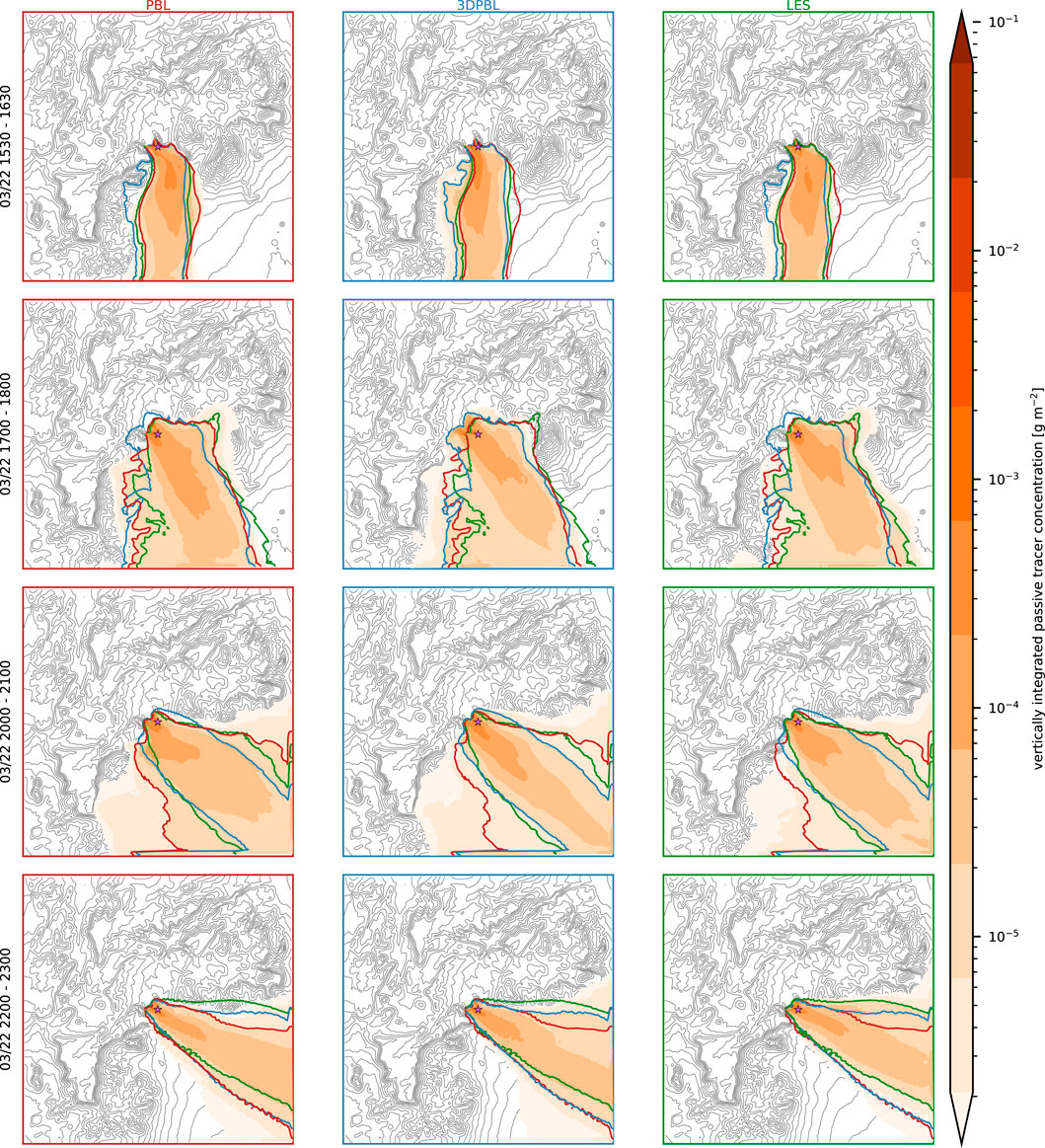
FIGURE 6. PBL, LES, and 3DPBL simulation results from D3 on March 22nd with filled contours of vertically integrated passive tracer concentration. Results are time-averaged over 1-h beginning at the start times of smoke releases. To assist with visually comparing the plumes, each subplot includes colored contour lines at 10⁻⁵ g·m⁻² from the three simulations with a red contour line from the PBL simulation, blue from the 3DPBL simulation, and green from the LES simulation. Gray contour lines represent topography with spacing of 50 m. A small purple star-shaped marker indicates the location of the P-tunnel apron. The results from D3, which is always configured with an LES SGS model, are shown, but the figure labels are according to the turbulence and mixing parameterization on the parent domain, D2.

FIGURE 7

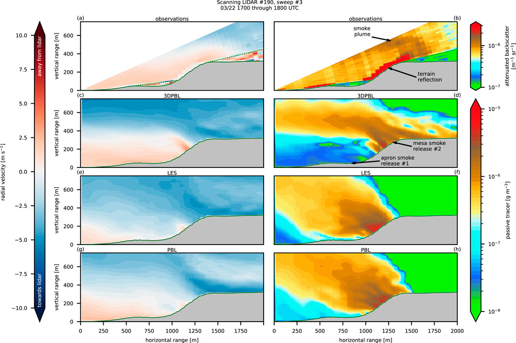
FIGURE 7. Observations of radial velocity (A) and attenuated backscatter (B) observed along sweep #3 by scanning lidar #190. Predictions from D3 of the 3DPBL, LES, and PBL simulations of radial velocity (C, E, G) and passive tracer concentration (D, F, H) along a transect defined by the scanning lidar sweep. Observations and predictions are time-averaged between 1700 and 1800 UTC on March 22nd. Note that the observations in (A,B) include nonphysical data in regions with obscured line of sight to the scanning lidar, indicated using dashed green lines. The surface of the mesa slope is distinguished by pronounced (i.e., bright red) attenuated backscatter in (B).

The observed radial velocity seen in Figure 7A shows flow above the mesa directed towards the lidar (northerly flow), while flow below the mesa is directed away from the lidar (southerly flow). This implies that the near surface flow is being locally driven in the valley, while flow over the mesa is synoptically driven. The three simulations produce similar flow patterns, shown in Figures 7C, E, G, but there are noteworthy differences between predicted wind speeds below the mesa and the heights at which the flow reverses. Positive radial velocities (southerly flow) below the mesa appear strongest in the 3DPBL simulation, and weakest in the LES simulation.

The flow reversal was also observed by instruments suspended by a tethered balloon flown from a flat location roughly 2 km south of the P-tunnel apron, 1 km south-southwest of scanning lidar #190, and with a surface elevation 350 m lower than the top of the mesa. The sensors on the tethersonde were flown at fixed heights, however, the balloon was grounded at 1810 UTC with the descent beginning at 1745 UTC. During the descent, the topmost anemometer detected the height flow reversal, which corresponds to a wind speed minimum. By fitting a curve to the wind speeds observed between 200 and 400 m AGL during the time of descent, the height of flow reversal above the tethersonde launch site is estimated at 316 m AGL, roughly 35 m below the elevation at the top of the mesa. Figure 8 includes vertical profiles of observed and predicted wind speed and wind direction, the fitted curves described above, and the approximated height of the flow reversal. When averaged between 1700 and 1800, the PBL, 3DPBL, and LES simulations predict heights of flow reversal at 303, 278, and 274 m AGL, respectively. The simulations all predict a flow reversal that is reasonably close to what was observed by the tethersonde.

FIGURE 8

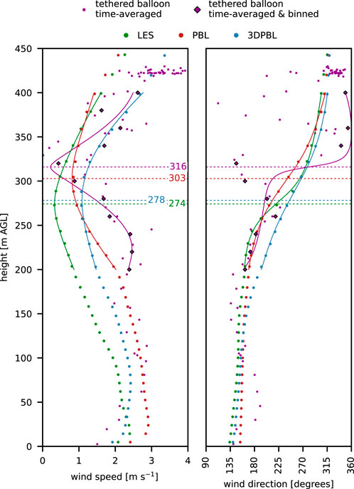
FIGURE 8. Vertical profiles of predicted and observed wind speed and wind direction at the launch site of tethered balloon. The predictions from D3 are time averaged between 1700 and 1800 UTC. Observations recorded during the balloon descent by the topmost sensor are averaged every 30 s and are shown with small purple circular markers. The 30 s averaged observations are grouped into bins with 20 m vertical spacing. The mean wind speed and wind direction within each 20 m bin are shown with a purple diamond markers. Third order polynomials are fit to the time-averaged predictions and to the averaged and binned observations between 200 and 400 m AGL. The height of the wind speed minimum, shown with a dashed horizontal line, is estimated from each fitted curve of wind speed.

Comparison of the vertical profiles in Figure 8 highlights the importance vertical grid resolution when simulating conditions involving high shear. Because of the steep mountainous slopes and the WRF model’s terrain-following vertical coordinate, further refining the near-surface vertical grid resolution introduces grid skewness resulting in numerical instability. These constraints further motivate the development of alternative gridding techniques within the WRF model that allow for highly resolved complex topography, such as the immersed boundary method (Lundquist et al., 2012; Arthur et al., 2018; Wiersema et al., 2020; Wiersema et al., 2022). Regardless of potential benefits from increased vertical grid resolution, all three simulations predict a pronounced wind speed minimum close to, within 50 m of, what was observed.

Each simulation produces a distinct wind speed profile, with no simulation clearly outperforming the others. The differences between predicted wind speed profiles once again indicates that the choice of turbulence and mixing parameterization applied in the terra incognita can have a significant impact on predictions, particularly when conditions are stable or local forcing is dominant. The PBL simulation is most visually consistent with the observations below 200 m AGL and most closely predicts the height of the wind speed minimum. The 3DPBL simulation has the best visual agreement with the observed wind speeds above 325 m AGL. The magnitude of the minimum wind speed predicted by each simulation also varies greatly, with the minimum of the fitted curve to the 3DPBL, PBL, and LES simulations at 1.08, 0.81, and 0.33 m·s⁻¹, respectively. The curve fitted to wind speed observations has a minimum of 0.22 m·s⁻¹. The tethered balloon observed some extremely quiescent conditions during descent, such as a 30 s average wind speed of 0.02 m·s⁻¹ at 329 m AGL.

Figure 7B shows the smoke plume transported over the mesa top after being released along the mesa edge. After traveling approximately 250 m downrange, the smoke plume rises, reverses direction, and is advected uprange (southeasterly) aloft of the P-tunnel apron and beyond the lidar scan-plane’s upper boundary. Of the three predicted plumes, the 3DPBL simulation appears most consistent with the observed transport and dispersion. While the PBL and LES simulation plumes do not extend far downrange beyond the mesa cliff edge, the 3DPBL simulation plume extends several hundred meters after the mesa edge. Concentrations predicted near-surface between scanning lidar #190 and the P-tunnel apron are notably lowest in the 3DPBL simulation. This particular instance exemplifies that the choice of turbulence and mixing parameterization for domains within the terra incognita can markedly influence near-source microscale predictions of transport and dispersion over complex terrain.

6.3 March 28th

March 28th is distinguished from the other 2 days simulated by lower average wind speeds. Shortly after local sunrise at 1335 UTC (6:35 a.m. local time), the flow transitions from north-northwesterly to southeasterly at all sites and elevations. As shown in Figure 9, the first smoke release on the 28th, beginning at 1400 UTC, advects southwards and downslope from the apron release locations while forming a narrow plume that is channeled by the terrain contours. Compared to the 21st and 22nd, plumes on the 28th persist for much longer within the modeling domain due to the low wind speeds and the early-morning transition in wind direction. Additionally, the start of the first release period (1400 UTC) begins earlier in the morning than on the 21st (1500 UTC) or the 22nd (1530 UTC), resulting in a release with more stable atmospheric conditions. These factors result in a noticeable amount of smoke from any prior releases lingering within the 25 km² domain (D3) during and after subsequent smoke releases.

FIGURE 9

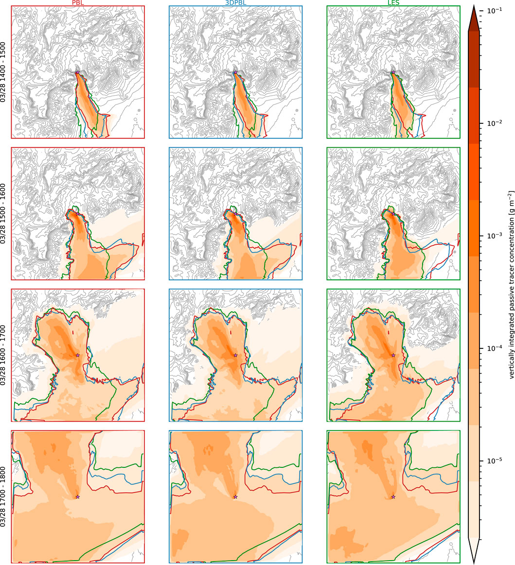
FIGURE 9. PBL, LES, and 3DPBL simulation results from D3 on March 28th with filled contours of vertically integrated passive tracer concentration. Results are time-averaged over 1-h beginning at the start times of smoke releases. To assist with visually comparing the plumes, each subplot includes colored contour lines at 10⁻⁵ g·m⁻² from the three simulations with a red contour line from the PBL simulation, blue from the 3DPBL simulation, and green from the LES simulation. Gray contour lines represent topography with spacing of 50 m. A small purple star-shaped marker indicates the location of the P-tunnel apron. The results from D3, which is always configured with an LES SGS model, are shown, but the figure labels are according to the turbulence and mixing parameterization on the parent domain, D2.

Particularly for the first three smoke releases on the 28th, differences between the predicted plumes are most pronounced over the relatively flat region in the southeast of D3. Following the morning transition from north-northwesterly to southeasterly flow, smoke is transported over higher terrain north of the P-tunnel apron and above the mesa top. These “arms” of the predicted plumes that reach northward are visually comparable with each other and show negligible differences between the three simulations.

Averaged between 1400 and 1500 UTC, the predicted plumes are narrow and visibly differ from each other only after reaching the flat region in the southeast of D3. This behavior can be attributed to the highly stable atmospheric conditions that inhibit mixing and results in shallow plumes constrained near the surface where they are strongly influenced by the complex topography. Altering the turbulence and mixing parameterization on D2 has a minimal impact on predictions until the smoke reaches the flat region where the plumes are less influenced by the complex terrain.

Between 1500 and 1600 UTC, the LES simulation produces a plume that is relatively narrow compared to the 3DPBL and PBL simulations, which both predict plumes that reach the east boundary of D3. Similar trends are seen between 1600 and 1700 UTC, with the highlighted contour level of 10⁻⁵ g·m⁻² from the LES simulation plume remaining distanced from the east boundary. Between 1700 and 1800 UTC, the predicted plumes elongate to the north and west, covering over the majority of D3, which stands in contrast to the plumes predicted on the 21st and 22nd that covered, at most, one quarter of D3.

7 Conclusion and ongoing research

Here we evaluated multiscale simulations of the METEX21 field campaign with an objective of developing insight into the choice of turbulence parameterization for domains within the terra incognita (i.e., the turbulence gray-zone). These simulations demonstrate that the method used to parameterize turbulence and mixing in the terra incognita can significantly influence microscale predictions of transport and dispersion, particularly when atmospheric conditions are locally forced. This influence was not apparent when analyzing the model skill for prediction of wind speed, wind direction, and turbulence kinetic energy, however, important differences between the simulations are revealed through a qualitative evaluation of transport and dispersion of smoke plume behavior. Follow up tracer release campaigns would greatly benefit from quantifiable tracer releases with robust sensing of tracer concentrations. Careful observation of a different tracer, such as SF₆ or a compound not found in the background environment, may highlight yet unseen differences between these simulation configurations that are not obvious when analyzing wind speed, wind direction, and TKE.

Additionally, these simulations provide insight into the performance of the new 3D PBL scheme of Juliano et al. (2022) relative to a traditional PBL scheme and LES closure model. The MYNN PBL scheme and TKE1.5 LES closure model were considered due to their frequency of use by the multiscale modeling community, while the 3D PBL scheme was considered as a promising development for intermediate resolution domains in the terra incognita. Here, the 3DPBL simulation best predicts transport and dispersion of the smoke plumes on March 22nd when conditions were predominantly locally forced within the valley and observed plume behavior was particularly complicated due to different wind directions based on elevation.

These simulations have a high computational cost, which has restricted the number of configurations and methods that are compared. There are many compelling methods to consider for evaluation in future studies, including the hybrid Reynolds Averaged Navier Stokes (RANS) and LES scheme of Senocak et al. (2007), which blends the LES solution with a RANS solution near boundaries where the characteristic length scale of turbulence is smaller than the grid resolution. Future work could also evaluate more advanced turbulence closure models, such as the dynamic reconstruction model (DRM) (Chow et al., 2005) or the nonlinear backscatter and anisotropy (NBA) model (Kosović, 1997; Mirocha et al., 2010).

Generalized conclusions are difficult to reach due to the inherent uniqueness of microscale meteorology over a location with complex terrain. These METEX21 simulations demonstrate that when synoptic forcing is dominant, the transport and dispersion is less impacted by changes to turbulence and flow features resolved in the terra incognita, relative to when local forcing is dominant. To gain broad insights into “best practices” in the terra incognita, additional modeling studies are necessary with a diversity of configurations, locations, and meteorological conditions.

Finally, these multiscale simulations emphasize some limitations of the WRF model, particularly regarding the methods for parallelization and gridding. Recently developed codes, such as the Energy Research and Forecasting (ERF) model (Almgren et al., 2023) and the FastEddy model (Sauer and Muñoz-Esparza, 2020), are highly optimized and can fully leverage modern high performance computing resources (i.e., hybrid CPU/GPU computing), enabling larger domains and higher resolutions while reducing wall-clock time. As these models mature and computing resources become more accessible, it is likely that multiscale modeling will become more commonplace and there will be increasing benefit from field campaigns for model validation and case studies for informing model configuration.

Data availability statement

The datasets presented in this article are not readily available because Data from the METEX21 field campaign is temporarily restricted and will become available after 2 years from the completion of the field campaign (27 July 2023). Sharing of model output produced in this study is currently unfeasible due to the large file sizes, approximately 30 terabytes total. Requests to access the datasets should be directed to DW, wiersema1@llnl.gov.

Author contributions

DW configured and analyzed the simulations, and drafted the manuscript. SW led the organization of the METEX21 field experiment, provided valuable insight about the observational datasets, and helped edit the manuscript. RA assisted with drafting the manuscript, assisted with simulation configuration and debugging, and provided code for scalar upscaling. TJ provided the 3D PBL code, assisted with simulation configuration and debugging, and helped draft the manuscript. KL and LG advised throughout this study, providing expertise regarding microscale meteorology and transport and dispersion. RN was diagnostic lead for the scanning lidars. WS was diagnostic lead for the meteorological towers. MB was diagnostic lead for the meteorological tripods. DD was diagnostic lead for the tethersonde. All authors contributed to the article and approved the submitted version.

Funding

This research was funded by the National Nuclear Security Administration, Defense Nuclear Nonproliferation Research and Development (NNSA DNN R&D). This work was performed under the auspices of the U.S. Department of Energy by Lawrence Livermore National Laboratory under Contract DE-AC52-07NA27344. This research was funded in part by the U.S. Department of Energy Office of Energy Efficiency and Renewable Energy Wind Energy Technologies Office. The National Center for Atmospheric Research is a major facility sponsored by the National Science Foundation under Cooperative Agreement 1852977.

Acknowledgments

The authors acknowledge important interdisciplinary collaboration with scientists and engineers from LANL, LLNL, MSTS, PNNL, and SNL. This manuscript will has been approved for external release (LLNL-JRNL-843907).

Conflict of interest

The authors declare that the research was conducted in the absence of any commercial or financial relationships that could be construed as a potential conflict of interest.

Publisher’s note

All claims expressed in this article are solely those of the authors and do not necessarily represent those of their affiliated organizations, or those of the publisher, the editors and the reviewers. Any product that may be evaluated in this article, or claim that may be made by its manufacturer, is not guaranteed or endorsed by the publisher.

References

Almgren, A., Lattanzi, A., Haque, R., Jha, P., Kosovic, B., Mirocha, J., et al. (2023). ERF: energy research and forecasting. J. Open Source Softw. 8, 5202. doi:10.21105/joss.05202

CrossRef Full Text | Google Scholar

Arthur, R., Lundquist, K., Mirocha, J., and Chow, F. K. (2018). Topographic effects on radiation in the WRF model with the immersed boundary method: implementation, validation, and application to complex terrain. Mon. Weather Rev. 146, 3277–3292. doi:10.1175/MWR-D-18-0108.1

CrossRef Full Text | Google Scholar

Arthur, R. S., Juliano, T. W., Adler, B., Krishnamurthy, R., Lundquist, J. K., Kosović, B., et al. (2022). Improved representation of horizontal variability and turbulence in mesoscale simulations of an extended cold-air pool event. J.Appl. Meteor. Climatol. 61, 685–707. doi:10.1175/jamc-d-21-0138.1

CrossRef Full Text | Google Scholar

Benjamin, S. G., Weygandt, S. S., Brown, J. M., Hu, M., Alexander, C. R., Smirnova, T. G., et al. (2016). A north american hourly assimilation and model forecast cycle: the rapid refresh. Mon. Weather Rev. 144, 1669–1694. doi:10.1175/MWR-D-15-0242.1

CrossRef Full Text | Google Scholar

Calhoun, R., Gouveia, F., Shinn, J., Chan, S., Stevens, D., Lee, R., et al. (2004). Flow around a complex building: comparisons between experiments and a Reynolds-averaged Navier-Stokes approach. J. Appl. Meteorology 43, 696–710. doi:10.1175/2067.1

CrossRef Full Text | Google Scholar

Chow, F. K., Schar, C., Ban, N., Lundquist, K. A., Schlemmer, L., and Shi, X. (2019). Crossing multiple gray zones in the transition from mesoscale to microscale simulation over complex terrain. Atmosphere 10, 274. doi:10.3390/atmos10050274

CrossRef Full Text | Google Scholar

Chow, F. K., Street, R. L., Xue, M., and Ferziger, J. H. (2005). Explicit filtering and reconstruction turbulence modeling for large-eddy simulation of neutral boundary layer flow. J. Atmos. Sci. 62, 2058–2077. doi:10.1175/JAS3456.1

CrossRef Full Text | Google Scholar

Daniels, M., Lundquist, K., Mirocha, J., Wiersema, D., and Chow, F. K. (2016). A new vertical grid nesting capability in the Weather Research and Forecasting (WRF) model. Mon. Weather Rev. 144, 3725–3747. doi:10.1175/MWR-D-16-0049.1

CrossRef Full Text | Google Scholar

Deardorff, J. W. (1980). Stratocumulus-capped mixed layers derived from a three-dimensional model. Boundary-Layer Meteorol. 18, 495–527. doi:10.1007/BF00119502

CrossRef Full Text | Google Scholar

Dudhia, J. (2022). Challenges in sub-kilometer grid modeling of the convective planetary boundary layer. Meteorology 1, 402–413. doi:10.3390/meteorology1040026

CrossRef Full Text | Google Scholar

Dudhia, J. (1989). Numerical study of convection observed during the winter monsoon experiment using a mesoscale two-dimensional model. J. Atmos. Sci. 46, 3077–3107. doi:10.1175/1520-0469(1989)046<3077:NSOCOD>2.0.CO;2

CrossRef Full Text | Google Scholar

Efstathiou, G. A., and Beare, R. J. (2015). Quantifying and improving sub-grid diffusion in the boundary-layer grey zone. Q. J. R. Meteorological Soc. 141, 3006–3017. doi:10.1002/qj.2585

CrossRef Full Text | Google Scholar

Ek, M., Mitchell, K., Lin, Y., Rogers, E., Grunmann, P., Koren, V., et al. (2003). Implementation of noah land surface model advances in the national centers for environmental prediction operational mesoscale eta model. J. Geophys. Res. Atmos. 108. doi:10.1029/2002JD003296

CrossRef Full Text | Google Scholar

Farr, T. G., Rosen, P. A., Caro, E., Crippen, R., Duren, R., Hensley, S., et al. (2007). The shuttle radar topography mission. Rev. Geophys. 45. doi:10.1029/2005RG000183

CrossRef Full Text | Google Scholar

Honnert, R., Efstathiou, G. A., Beare, R. J., Ito, J., Lock, A., Neggers, R., et al. (2020). The atmospheric boundary layer and the “gray zone” of turbulence: a critical review. J. Geophys. Research-Atmospheres 125. doi:10.1029/2019JD030317

CrossRef Full Text | Google Scholar

Hu, X.-M., Nielsen-Gammon, J. W., and Zhang, F. (2010). Evaluation of three planetary boundary layer schemes in the wrf model. J. Appl. Meteorology Climatol. 49, 1831–1844. doi:10.1175/2010JAMC2432.1

CrossRef Full Text | Google Scholar

Jiménez, P. A., Dudhia, J., González-Rouco, J. F., Navarro, J., Montávez, J. P., and García-Bustamante, E. (2012). A revised scheme for the wrf surface layer formulation. Mon. Weather Rev. 140, 898–918. doi:10.1175/MWR-D-11-00056.1

CrossRef Full Text | Google Scholar

Juliano, T., Kosović, B., Munoz, P. J., Eghdami, M., Haupt, S. E., and Martilli, A. (2022). Gray zone simulations using a three-dimensional planetary boundary layer parameterization in the Weather Research and Forecasting model. Mon. Weather Rev. 150, 1585–1619. doi:10.1175/MWR-D-21-0164.1

CrossRef Full Text | Google Scholar

Kosović, B., Munoz, P. J., Juliano, T. W., Martilli, A., Eghdami, M., Barros, A. P., et al. (2020). Three-dimensional planetary boundary layer parameterization for high-resolution mesoscale simulations. J. Phys. Conf. Ser. 1452, 012080. doi:10.1088/1742-6596/1452/1/012080

CrossRef Full Text | Google Scholar

Kosović, B. (1997). Subgrid-scale modelling for the large-eddy simulation of high-Reynolds-number boundary layers. J. Fluid Mech. 336, 151–182. doi:10.1017/S0022112096004697

CrossRef Full Text | Google Scholar

Lundquist, K., Chow, F. K., and Lundquist, J. (2012). An immersed boundary method enabling large-eddy simulations of flow over complex terrain in the WRF model. Mon. Weather Rev. 140, 3936–3955. doi:10.1175/MWR-D-11-00311.1

CrossRef Full Text | Google Scholar

Mellor, G. L., and Yamada, T. (1974). A hierarchy of turbulence closure models for planetary boundary layers. J. Atmos. Sci. 31, 1791–1806. doi:10.1175/1520-0469(1974)031<1791:ahotcm>2.0.co;2

CrossRef Full Text | Google Scholar

Mellor, G. L., and Yamada, T. (1982). Development of a turbulence closure model for geophysical fluid problems. Rev. Geophys. 20, 851–875. doi:10.1029/rg020i004p00851

CrossRef Full Text | Google Scholar

Meneveau, C., and Katz, J. (2000). Scale-invariance and turbulence models for large-eddy simulation. Annu. Rev. Fluid Mech. 32, 1–32. doi:10.1146/annurev.fluid.32.1.1

CrossRef Full Text | Google Scholar

Mirocha, J., Lundquist, J., and Kosović, B. (2010). Implementation of a nonlinear subfilter turbulence stress model for large-eddy simulation in the advanced research WRF model. Mon. Weather Rev. 138, 4212–4228. doi:10.1175/2010MWR3286.1

CrossRef Full Text | Google Scholar

Mlawer, E. J., Taubman, S. J., Brown, P. D., Iacono, M. J., and Clough, S. A. (1997). Radiative transfer for inhomogeneous atmospheres: rrtm, a validated correlated-k model for the longwave. J. Geophys. Res. Atmos. 102, 16663–16682. doi:10.1029/97JD00237

CrossRef Full Text | Google Scholar

Muñoz-Esparza, D., and Kosović, B. (2018). Generation of inflow turbulence in large-eddy simulations of nonneutral atmospheric boundary layers with the cell perturbation method. Mon. Weather Rev. 146, 1889–1909. doi:10.1175/mwr-d-18-0077.1

CrossRef Full Text | Google Scholar

Muñoz-Esparza, D., Kosović, B., Mirocha, J., and van Beeck, J. (2014). Bridging the transition from mesoscale to microscale turbulence in numerical weather prediction models. Boundary-Layer Meteorol. 153, 409–440. doi:10.1007/s10546-014-9956-9

CrossRef Full Text | Google Scholar

Muñoz-Esparza, D., Kosović, B., van Beeck, J., and Mirocha, J. (2015). A stochastic perturbation method to generate inflow turbulence in large-eddy simulation models: application to neutrally stratified atmospheric boundary layers. Phys. Fluids 27. doi:10.1063/1.4913572

CrossRef Full Text | Google Scholar

Nagel, T., Schoetter, R., Masson, V., Lac, C., and Carissimo, B. (2022). Numerical analysis of the atmospheric boundary-layer turbulence influence on microscale transport of pollutant in an idealized urban environment. Boundary-Layer Meteorol. 184, 113–141. doi:10.1007/s10546-022-00697-7

CrossRef Full Text | Google Scholar

Nakanishi, M., and Niino, H. (2006). An improved mellor–yamada level-3 model: its numerical stability and application to a regional prediction of advection fog. Boundary-Layer Meteorol. 119, 397–407. doi:10.1007/s10546-005-9030-8

CrossRef Full Text | Google Scholar

Peña, A., and Hahmann, A. (2020). Evaluating planetary boundary-layer schemes and large-eddy simulations with measurements from a 250-m meteorological mast. J. Phys. Conf. Ser. 1618, 062001. doi:10.1088/1742-6596/1618/6/062001

CrossRef Full Text | Google Scholar

Sauer, J. A., and Muñoz-Esparza, D. (2020). The fasteddy® resident-gpu accelerated large-eddy simulation framework: model formulation, dynamical-core validation and performance benchmarks. J. Adv. Model. Earth Syst. 12, e2020MS002100. doi:10.1029/2020MS002100

CrossRef Full Text | Google Scholar

Senocak, I., Ackerman, A. S., Kirkpatrick, M. P., Stevens, D. E., and Mansour, N. N. (2007). Study of near-surface models for large-eddy simulations of a neutrally stratified atmospheric boundary layer. Boundary-Layer Meteorol. 124, 405–424. doi:10.1007/s10546-007-9181-x

CrossRef Full Text | Google Scholar

Skamarock, W. C., Klemp, J. B., Dudhia, J., Gill, D. O., Liu, Z., Berner, J., et al. (2021). A description of the advanced research WRF version 4.3. Technical note NCAR/TN-556+STR. United States: National Center for Atmospheric Research. doi:10.5065/1dfh-6p97

CrossRef Full Text | Google Scholar

Smagorinsky, J. (1963). General circulation experiments with the primitive equations: I. The basic experiment. Mon. Wea. Rev. 91, 99–164. doi:10.1175/1520-0493(1963)091<0099:gcewtp>2.3.co;2

CrossRef Full Text | Google Scholar

Smagorinsky, J. (1993). “Some historical remarks on the use of nonlinear viscosities,” in Large eddy simulation of complex engineering and geophysical flows, Proceedings of an international workshop in large eddy simulation. Editors B. Galperin, and S. A. Orszag (Cambridge, UK: Cambridge University Press), 3–36.

Google Scholar

Thompson, G., and Eidhammer, T. (2014). A study of aerosol impacts on clouds and precipitation development in a large winter cyclone. J. Atmos. Sci. 71, 3636–3658. doi:10.1175/JAS-D-13-0305.1

CrossRef Full Text | Google Scholar

Wiersema, D., Lundquist, K., and Chow, F. K. (2020). Mesoscale to microscale simulations over complex terrain with the immersed boundary method in the Weather Research and Forecasting model. Mon. Weather Rev. 148, 577–595. doi:10.1175/MWR-D-19-0071.1

CrossRef Full Text | Google Scholar

Wiersema, D., Lundquist, K., Mirocha, J., and Chow, F. K. (2022). Evaluation of turbulence and dispersion in multiscale atmospheric simulations over complex urban terrain during the joint urban 2003 field campaign. Mon. Weather Rev. 150, 3195–3209. doi:10.1175/MWR-D-22-0056.1

CrossRef Full Text | Google Scholar

Wyngaard, J. (2004). Toward numerical modeling in the “terra incognita”. J. Atmos. Sci. 61, 1816–1826. doi:10.1175/1520-0469(2004)061<1816:tnmitt>2.0.co;2

CrossRef Full Text | Google Scholar