 Sonia Wharton1*
 Michael J. Brown2
 Darielle Dexheimer3
 Jerome D. Fast4Rob K. Newsom4Walter W. Schalk5
 David J. Wiersema1
- 1Lawrence Livermore National Laboratory, Livermore, CA, United States
- 2Los Alamos National Laboratory, Los Alamos, NM, United States
- 3Sandia National Laboratories, Albuquerque, NM, United States
- 4Pacific Northwest National Laboratory, Richland, WA, United States
- 5National Oceanic and Atmospheric Administration, Air Resources Laboratory, Special Operations and Research Division, Las Vegas, NV, United States
METEX21 was an atmospheric tracer release experiment executed at the Department of Energy’s Nevada National Security Site (NNSS) in the southwestern U.S to study terrain-induced wind and thermodynamic conditions that influence local-scale (<5-km) plume transport under varying atmospheric forcing conditions. Meteorological observations were collected using 10-m tall meteorological towers, 2-m tall tripods with 3-d sonic anemometers, a 3-m tall eddy covariance flux tower, Doppler profiling lidars, Doppler scanning lidars, weather-balloon launched radiosondes, and a tethered balloon equipped with wind, temperature, and aerosol sensors at heights up to 800 m. A smoke tracer was released along three transects in the horizontal and vertical directions and observed with video cameras, aerosol sensors and lidars (via aerosol backscatter). The observations showed evidence of large-scale/synoptic transience as well as local-scale upslope and downslope flows, along-axis valley flows, recirculation eddies on leeward slopes, and periods of strong shear and veer aloft. The release days were classified as either synoptically-driven or locally-driven, and a single case day is presented in detail for each. Synoptically-forced days show relatively narrow smoke plumes traveling down the valley from north to south (with the predominant wind direction), with little deviation in transport direction regardless of the elevation or ground locations of the smoke releases, except near the presence of leeside recirculation eddies. Locally-forced days exhibit a wider range of plume behavior due to the combination of thermally-induced valley and slope flows, which are often flowing in different cardinal directions, and wind shear found aloft at higher altitudes and elevations. We saw evidence of smoke lofting on top of the mesas due to strong upslope flows on these days. A major finding of this experiment was the effectiveness of scanning lidars to measure 2-dimensional plume transport out to a 2–3 km distance; much farther than could be visibly observed. METEX21 was the first of three planned tracer experiments at NNSS, and future experiments will incorporate multiple tracers to improve individual plume identification so that finer resolution flow details can be attained from these measurements, as well as deploy a larger suite of meteorological instrumentation, including more temperature profiling data.
1 Introduction
Transport and dispersion of tracers in the atmosphere is primarily driven by the mean wind field; however, other factors including terrain, mechanical turbulence, vertical mixing (i.e., thermal turbulence), the height of the surface layer and planetary boundary layer (PBL), entrainment, precipitation, and tracer chemistry all play a role in plume behavior. Atmospheric dispersion and transport experiments have been conducted at least since the 1950’s for military and civilian purposes. With the advent of national air quality standards in the 1960’s interest shifted to tracking the long-range or regional transport of human-health pollutants, and tracer release experiments were designed at those scales. Over time transport and dispersion experiments have evolved to include finer-resolution urban and complex terrain environments, including looking at the transport of tracers through urban city canyons (e.g., Joint Urban 2003, Allwine and Flaherty, 2006; DAPPLE, Martin et al., 2010), the coastal sea breeze-city interface (e.g., TexAQS II, Parrish et al., 2009), complex/coastal terrain (e.g., DOPPTEX, Thuillier, 1992; Nasstrom et al., 2007), and complex/mountain terrain (e.g., ASCOT, Orgill and Schreck, 1985; ASCOT-Colorado/Rocky Flats Plant, Poulos and Bossert, 1995, Banta et al., 1996; TRACT, Fiedler and Borrell, 2000). Conducting experiments at finer scales has also been driven by the need to validate the next-generation of multiscale atmospheric models, which simulate flow at scales ranging from mesoscale (>1 km) to meter-scale.
A handful of these dispersion and transport experiments are considered “classical experiments” and are important to this day for atmospheric model validation. However, measurement and modeling uncertainties in plume behavior remain and warrant additional tracer release experiments, especially as models now simulate down to the meter-scale resolution. These uncertainties are especially large for air motion and tracer transport over locally (defined here as 5 km or less) complex terrain. At this distance the scales of interest overlap the microscale and mesoscale and include the interactions between local topography and surface-atmospheric boundary layer physics with larger-scale meteorological forcing. For example, locally complex terrain creates strong heterogeneity in the horizontal and vertical flow fields over relatively small distances, which results in individual observations being representative of limited spatial and temporal extents. This is especially true if multiple plumes from different source locations or elevations are emitted simultaneously in mountain terrain where local features strongly affect the flow and plume transport. This can have large implications for how we interpret and react to national security and human health incidents.
Repeated experiments and multiple instrument platforms are still needed to gather data under locally varying terrain environments. To address this, a 5 km long by 2 km wide domain at the northern end of the Nevada National Security Site (NNSS) was chosen for a series of meteorological and tracer release experiments conducted by the U.S. Department of Energy. The Meteorology Experiment (METEX21) is the first of three tracer release experiments to study the impacts of complex terrain and flow features on plume dispersion and transport. A second field campaign was completed in October 2022 and focused on the release of a radiotracer alongside smoke. A third experiment is planned for 2025 and will have a more extensive array of radiotracers (e.g., dual tracer releases) and meteorological instrumentation, including more temperature profiling sensors.
Specific goals of METEX21 were to:
1) examine the utility of different meteorological instruments in locally complex terrain to optimally capture the complex flow field, including up-valley and down-valley and upslope and downslope flows. This includes evaluating what instruments are needed to capture flow across our vertical and horizontal distance scales, where these instruments should be placed in the experimental domain and testing of different lidar scanning strategies to capture wind flow and plume behavior.
2) examine how release locations, as a function of elevation and ground distance, affect plume transport in an area that is locally complex. The smoke transects were designed to study how release elevation affects plume transport as well as the effects of horizontal distance separating release points.
3) provide a robust dataset of multi-day atmospheric observations to validate atmospheric transport and diffusion models across the microscale-mesoscale interface.
This paper serves as an overview of the METEX21 field campaign and describes the instrumentation and smoke release execution. Observations from two case days are highlighted to emphasize how local terrain and tracer release height influences plume transport under different atmospheric forcing conditions. These include a day dominated by synoptic forcing and consistent northerly winds (March 21) and a day with local (e.g., diurnal surface heating) forcing and strong wind veer found between the valley flow and flow aloft (March 22). For readers interested in the atmospheric modeling of these days, those results and discussion are found in Wiersema et al. (2023).
2 Site description
METEX21 took place along and on top of a mesa, called the Aqueduct Mesa, and along a narrow, 5-km long valley, that is referred to here as the “P-tunnel valley.” The overall terrain slopes from north to south starting at the higher elevation Aqueduct Mesa and P-tunnel apron in the north, to the lower elevation, broader Yucca Flat in the south. Hills and mesas are found along the edges of P-tunnel valley. The P-tunnel apron is defined as the relatively flat, 300-m wide area at the base of Aqueduct Mesa which serves as the entry point for a tunnel called the P tunnel. A photograph of this landscape taken from Aqueduct Mesa is shown in Figure 1. Idealized, terrain-induced flow patterns and the apron meteorological tower/smoke release locations are also shown.
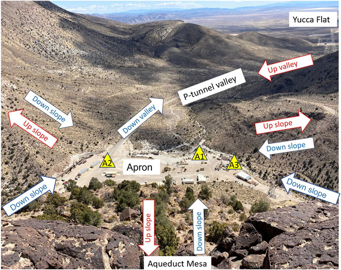
FIGURE 1. Photograph taken from Aqueduct Mesa at mesa edge release location #2 (M2) facing south and overlooking the apron, P-tunnel valley, and much larger Yucca Flat valley. The apron smoke release locations are shown and labeled (A1, A2 and A3). Also visible are the two terminating canyons and local hills and ridgelines in the immediate vicinity of the apron. Idealized flow directions are shown for locally-driven flow: daytime winds flow up-valley or upslope, and nighttime drainage winds are down-valley or downslope.
Elevations range from 1950 m a.s.l. on top of Aqueduct Mesa to 1,490 m a.s.l. at the southern end of our domain in Yucca Flat. These elevations result in two dominant ecosystems: a piñon pine/juniper woodland on the mesa tops and slopes, and a blackbrush/sagebrush shrub steppe in the valley below. Both ecological communities are typical of the U.S. Great Basin Desert.
3 Materials and methods
3.1 Experiment planning
METEX21 was designed around a preference for northerly winds, i.e., winds from the north. Due to site boundaries, we were not able to deploy sensors and towers more than a few kilometers north of the smoke release points. For this reason, the experiment was executed in early spring (March) to take advantage of daytime northerly winds that were climatologically predicted with moderate frequency. We also targeted a time of year that had a lower probability of deep snow cover on top of Aqueduct Mesa (for access purposes), extensive cloud cover (for analyzing the smoke video footage), and significant precipitation.
At NNSS in March, the weather is shifting from being dominated by the winter-time Great Basin High circulation to the summer-time Thermal Low circulation. With this weather pattern shift comes a change in how the local winds at NNSS are forced, how strong they are, and which wind direction is prevalent during the daytime hours. Winds are driven by either synoptic meteorology or by local diurnal heating depending on the dominant forcing mechanism found on the day in question. Often, daytime flow in early spring is dominated by synoptic weather systems and winds are from the north, e.g., a cold frontal passage system, at all hours of the day. However, southerly winds are also found the day ahead of these northerly frontal passages, or on days with enough solar heating to create land-air-gradient local-forcing. Differential cooling and heating in this sloped terrain in combination with low humidities and clear skies, is a strong contributor to the overall flow pattern on days without strong synoptic forcing. These days are instead locally-forced, and an along-axis valley circulation pattern develops in the P-tunnel valley which is connected to the larger and broader Yucca Flat area. Down-valley (north to south) flows develop at night and persist into the early morning. Up-valley (south to north) flows develop soon after sunrise and last until near dusk. Valley thermal winds are usually much weaker than synoptically-forced nighttime winds. More information about the long-term climatology and wider-scale wind flow patterns found at NNSS is described in Soule (2006).
Although less well characterized prior to METEX21, slope flows were also expected to occur in the domain. Slope flows are caused by a temperature differential between the (non-flat) ground surface and atmosphere (i.e., the ground typically cools and heats at a faster rate) and the subsequent buoyancy forces produced. Topographic shading can also enhance these buoyancy forces. Slope flows were expected to be present near the edge of Aqueduct Mesa and on the P-tunnel apron which is at a higher elevation than the valley below. Flow on the apron was expected to be highly variable given the complexity of the immediate area. The apron is the terminus for two small canyons which define the western and eastern edges of Aqueduct Mesa. Recirculation, or rotor flows, were also predicted to occur on the leeward slopes near the apron.
Planning for each day’s smoke experiment included day-before and day-of weather forecasts provided by the Air Resources Laboratory/Special Operations Research Division (ARL/SORD). Forecasted days with lack of precipitation and cloud cover were given priority for releases. Due to the white color of the smoke, clear skies were preferred for the video footage. Local time during the experiment was Pacific Daylight Time (PDT), or UTC-7.
3.2 Instrumentation
Figure 2 shows the regional and local areas of interest. Our experimental domain extended out to 5-km from north-to-south, and vertically up through the tropopause, although the bulk of observations were taken at altitudes of 1 km or lower and lie in the PBL. Smoke was released on 7 days during the nine-day experiment. Deployed instruments for METEX21 included eleven 10-m tall meteorological towers (MT), six 2-m tall tripods with 3-d sonic anemometers (TT), one 3-m tall eddy covariance flux tower (BB), three Doppler profiling lidars (PL), two Doppler scanning lidars (SL), weather-balloon launched radiosondes (RS), and a tethered balloon system (TBS) equipped with wind, temperature, and aerosol sensors at multiple heights up to 800 m. Additionally, ARL/SORD regularly operates a mesonet network consisting of twenty-five 10 m tall towers across the NNSS site (https://www.sord.nv.doe.gov/index.php) and a sodar (Figure 2A) at the very southern end of NNSS and those data were included in the study. The METEX21 instruments were focused along the P-tunnel valley (Figure 2B), although a handful of instruments were also deployed on top of Aqueduct Mesa. Note that a higher density of towers and sensors was placed within the first kilometer south of the smoke release points due to the complexity of the terrain in that area (Figure 2C). The smoke release locations are also shown in Figure 2C. Details about each tower or sensor are listed in the sections below. Table 1 defines the instrumentation naming convention. A day-by-day overview of the executed release scenarios and instrumentation in operation is listed in Table 2.
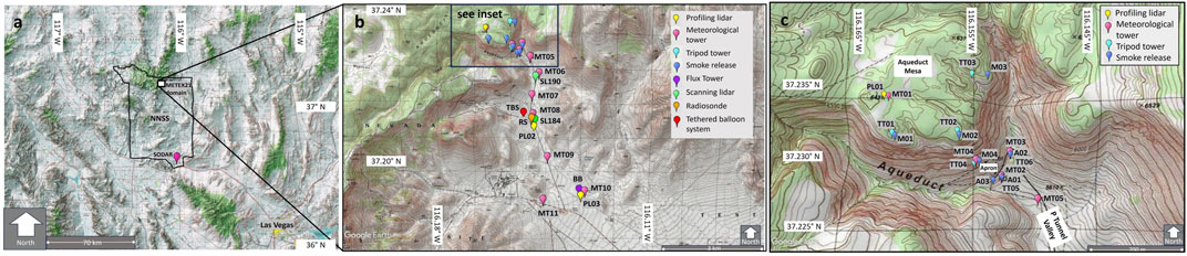
FIGURE 2. (A) Regional map of southern Nevada showing the Nevada National Security Site (NNSS) located northwest of the city of Las Vegas and locations of the METEX experiment domain and NNSS sodar. (B) Map of the METEX21 instrumentation showing all of the deployed instruments and sensors in the 5-km domain. (C) Detailed map of the northern section of the METEX21 domain showing the apron and mesa instrumentation and smoke release locations.
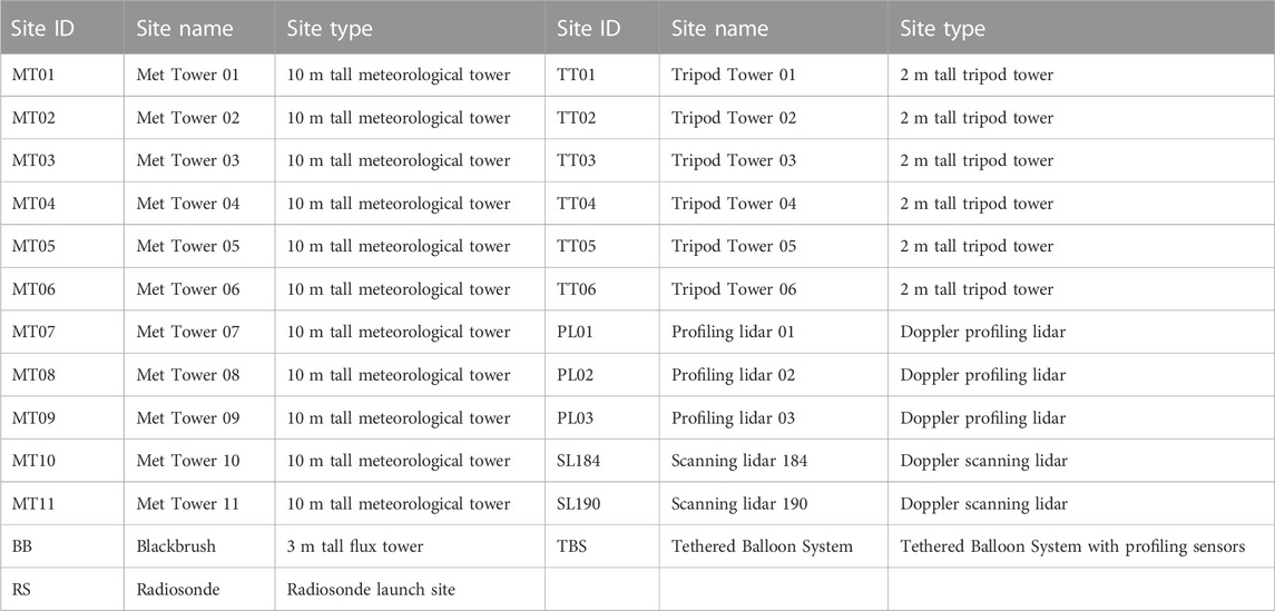
TABLE 1. Instrument site naming convention.
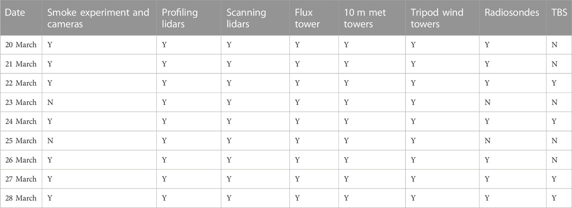
TABLE 2. Daily schedule during METEX21 showing which instrument platforms were operational and on which days the smoke releases occurred.
3.2.1 Smoke releases
Over 2,000 Superior Smoke 3C candles were ignited. Each candle contained approximately 40,000 cubic feet of dense white smoke which was emitted for approximately 3 min (release rate of 13,333 ft3/min). Each 30-minute smoke release was done by igniting five sets of either three (March 20–24, release rate of 40,000 ft3/min) or five (March 26–28, release rate of 66,666 ft3/min) candles. Each candle set was manually lit. 34 smoke release experiments were done across 7 days. Each smoke experiment was done as either a vertical transect or horizontal transect or a combination of both. The horizontal transects consisted of three release locations on the P tunnel apron (called the Apron Transect, A01-03) or three release locations along the Aqueduct Mesa edge (called the Mesa Edge Transect, M01-03) (Figure 2C). The Apron Transect covered a ground distance of 300 m. The Mesa Edge Transect covered a ground distance of 1 km. A vertical transect consisted of three release locations across a 270 m elevation gradient from the P tunnel apron to the top of the Aqueduct Mesa (called the Vertical Transect, A01, M04 and M02). On March 21 the Horizontal and Vertical Transects were done simultaneously. On March 26 the Vertical Transect releases were done at a higher time frequency and the release points were done in series to test the scanning lidar’s ability to pinpoint the individual plume source location. The Mesa Edge Transect release on March 27 was planned in a similar manner. Our smoke release times were constrained to daylight hours. Releases began as early as 0700 local time (PDT) and ended as late as 1630 local time (PDT). Further details on each release scenario are listed in Tables 3–5.
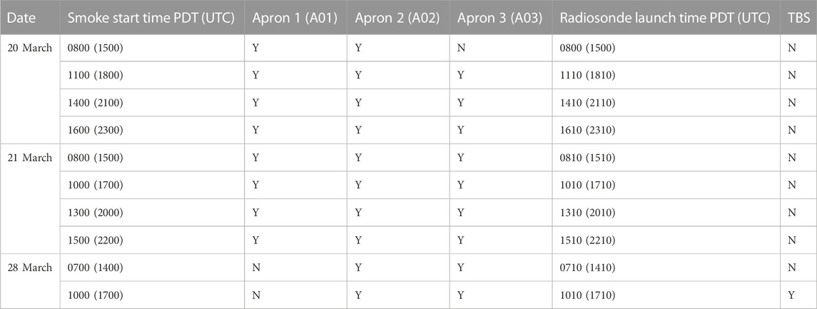
TABLE 3. Details for the Apron Transect releases. Also included is information on the weather-balloon radiosonde release time and whether the TBS was flown.
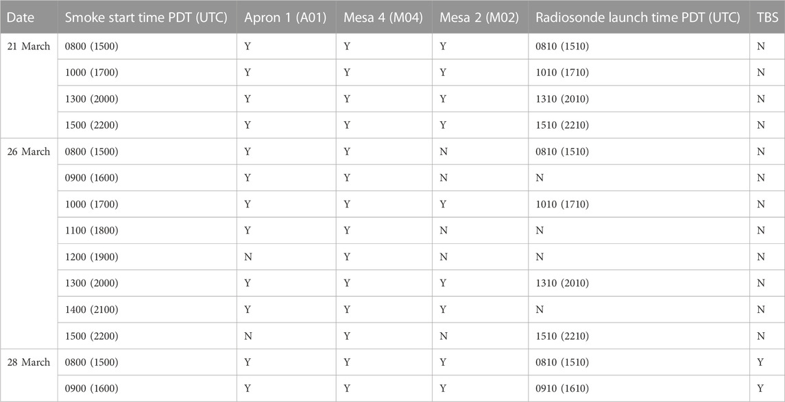
TABLE 4. Details for the Vertical Transect releases. Also included is information on the radiosonde release time and whether the TBS was flown.
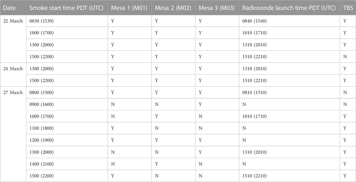
TABLE 5. Details for the Mesa Edge Transect releases. Also included is information on the radiosonde release time and whether the TBS was flown.
3.2.2 Meteorological towers and tripods
The three-dimensional wind vectors, u, v, and w (m/s) were measured at seventeen locations during METEX21 at high sampling resolution (10 Hz or greater) using 3-d sonic anemometry at the top of 10 m tall meteorological towers (MT01-11) and 2 m tall tripod towers (TT01-06). The anemometers included model RM Young 81000VRE (RM Young Company, USA) at the met towers and model RM Young model 81,000 at the tripod towers. From these data 10- and 15-minute average horizontal wind speed (U, m/s), direction (°), and turbulence kinetic energy (TKE, m2/s2) were calculated. The high frequency data were archived for additional variables, such as the momentum flux and sensible heat flux (using sonic temperature) calculations. The 10 m tall towers additionally measured 1 Hz air temperature (Ta, °C) and relative humidity (RH, %) (at two levels, 1.7 and 8.6 m), air pressure (P, kPa) (at 1.2 m), and incoming solar radiation (W/m2) (at 1.7 m) using a pyranometer. These variables were also averaged over a 10- and 15-minute period. The 10-minute average allowed for direct comparison to the profiling lidars; the 15-minute average allowed for comparison to the ARL/SORD mesonet towers. All except for MT01 were deployed on trailers. The trailer towers were aligned in a transect from north to south along the P-tunnel valley (see Figure 2B). A more permanent tower (MT01) was installed on Aqueduct Mesa and is now part of the ARL/SORD mesonet network (Figure 2C). MT01 was programmed to collect the same variables as the trailer towers, but only saved the 15-minute averages due to logistical constraints with telemetry on the mesa. The 2 m tall tripods were co-located with all but one of the smoke release locations: three tripods were along the Aqueduct Mesa edge (TT01-03) (co-located with M01-03), one on the Mesa slope (TT04) (co-located with M04), and two on the P-tunnel apron (TT05-06) (co-located with A01-02) (Figure 2C). Smoke release location A03 was a last-minute addition to the experiment and did not have a co-located 2 m tall tripod.
3.2.3 Flux tower
A 3 m tall eddy covariance flux tower called Blackbrush (BB), named after the dominant vegetation (mean canopy height ∼0.4 m), was deployed at the southern end of the 5-km METEX21 domain in Yucca Flat (Figure 2B) and collected 10 Hz measurements of u, v, and w-wind components and scalar (CO2, H2O vapor) densities. as well as 1 Hz measurements of Ta/RH, P, the solar radiation fluxes (incoming and outgoing shortwave and longwave radiation: kin, kout, lin, lout, W/m2), soil moisture (θv, m3/m3), and soil temperature (Ts, °C). Ts is an integrated measurement at depth of 0–15 cm; θv is taken at 8 cm. The ground measurements are done in replicas of four around the tower. The ground heat flux (G, W/m2) is estimated with four buried ground heat flux plates, each at a depth of 15 cm. The Blackbrush tower is equipped with an IRGASON sensor (Campbell Scientific, Inc., USA) at a height of 2.8 m for collecting the 3-axis wind components and densities of water vapor and carbon dioxide at 10 Hz over the plant and soil ecosystem. From these measurements the sensible heat flux (H, W/m2) and latent heat flux (LE, W/m2) are derived using the eddy covariance method (e.g., Baldocchi, 2003). The energy fluxes are calculated across a 30-min averaging period using the EasyFlux DL flux code (Campbell Scientific, Inc.) which includes standard correction procedures and algorithms typically used in the eddy covariance method. These include: 1) 10 Hz data were despiked and filtered using the sonic and gas analyser diagnostic codes, and signal strength and measurement output range thresholds 2) coordinate rotation was done using the double rotation method, 3) a lag correction was applied between CO2 and H2O measurements and the wind measurements, 4) frequency corrections were applied using cospectra and transfer functions of block averaging, and 5) a correction for air density changes was done using the WPL equations.
The energy fluxes (H, LE, G), with the inclusion of a calculated ground storage term (SG, W/m2), comprise the energy budget for the desert ecosystem. In practice, the amount of energy leaving a system should equal the amount of energy entering a system (at least when including energy storage and averaging over an extended period); however, the individual energy fluxes are measured using different instruments which varies the temporal sampling frequency and size and shape of the measurement area (i.e., the footprint). When checking for full energy closure, we determined that the energy budget at BB is close to 90% and is well within the acceptable and expected range for the eddy covariance method (Mauder et al., 2020). We note however that the eddy covariance method relies on a set of assumptions including horizontal homogeneity and net zero advection. Our tower location was purposely set in the flattest part of our experimental domain, however the mountains to the west and east of our tower likely produce some non-zero advection, especially at night. Users of the flux data should take this into consideration, especially if the nighttime CO2 fluxes (i.e., respiration fluxes) are studied for quantifying net ecosystem exchange (i.e., carbon balance calculations). For now, the 90% energy closure provided confidence that our surface energy fluxes were largely accounted for. The flux tower also provides an estimate of surface layer atmospheric stability via the scaling parameter, Obukhov length (L, m), which in combination with the temperature and wind profiles obtained from the launched radiosondes and tethered balloon provide a reasonably accurate assessment of atmospheric stability in the lower planetary boundary layer over the valley. The Obukhov length stability thresholds used here are based on those found in Panofsky and Dutton (1984) and Stull (1988).
3.2.4 Laser detection and ranging (lidar)
METEX21 utilized both profiling and scanning Doppler lidar to measure the wind vectors. The profiling lidars (PL) provided height- and time-resolved measurements of wind speed and direction. The scanning lidars (SL) provided range- and time-resolved measurements of radial (line-of-sight) velocity, attenuated backscatter, and wide-band signal-to-noise ratio (wSNR). While the beam positions in the profiling lidars are not programmable, the scanning lidars allow a wide array of scans to be performed, including the Plan Position Indicator (PPI) and Range Height Indicator (RHI) scans. Additionally, the scanning capability provided valuable information on the location, vertical extent, and concentration of the smoke plume. Because one of our primary objectives in METEX21 was to determine how to best use and program scanning lidars in complex terrain for plume detection, information about these instruments and their set-up is given in finer detail.
Lidars are sensitive to particulates (and insensitive to molecular scattering), and most of the signal is coming from the backscattering from aerosols in the atmosphere. Because the PBL over NNSS and this part of the country is relatively clear of natural- and man-made aerosols, the maximum lidar ranges that we were able to achieve were limited to out to 2–3 km for the scanning lidar. However, the clean background air acted in our favor for the capture of the smoke plumes as we saw distinct increases in wSNR in the lidar scans that could be attributed to smoke aerosols and thus, plume transport.
Three profiling lidars were deployed. These included one Windcube v2 (PL01) (Leosphere, France) and two ZephIR300s (PL02, PL03) (Zephir Ltd., England). Profiling lidars have the ability to penetrate the first couple hundred meters of the PBL, but no higher. The Windcube v2 uses a standard pulsed laser for ranging, whereas the ZephIR uses a focused continuous wave laser to provide range-resolved measurements. The Windcube v2 uses a Doppler Beam Swinging (DBS) method, and the ZephIR uses a Velocity Azimuth Display (VAD) method for computing the winds. The Windcube v2 is much more sensitive to low background aerosol count because it utilizes 4 laser beams to retrieve u and v, and a 5th beam to measure w while the ZephIR300 uses 55 beams across the cone scan. Thus, data availability for PL01 was often lower than for PL02 or PL03. In addition to the wind profiles, the Windcube v2 also provides vertical profiles of carrier-to-noise ratio, which is proportional to the backscatter. Thus, PL01 provided an additional location with potential smoke plume information. An additional advantage of the Windcube v2 is that it requires less power and was operated using a solar/battery array on top of the Mesa. The ZephIR lidars were run using gasoline generators. The profiling lidars were orientated to true north using multiple compasses and GPS units to find agreement.
PL01 was deployed on top of Aqueduct Mesa, PL02 was deployed 2 km from the base of the Mesa in the P tunnel valley, and PL03 was deployed at the very south end of our 5-km domain in Yucca Flat near MT10 and the BB flux tower, as indicated in Figure 2B. PL02 and PL03 were configured to collect wind data from 10 to 150 m a.g.l., at ten programmable heights. PL01 collected data from 40 to 150 m a.g.l., at twelve programmable heights. Note that the ZephIRs (PL02 and PL03) have a lower minimum measurement height due to the focused-continuous wave ranging method. Average wind speed, direction, and TKE were calculated across a 10-minute averaging period from the high-frequency data for both profiling lidar models. Although profiling lidars assume a set of ideal atmospheric flow conditions (e.g., horizontal homogeneity in the scan volume) to derive wind speed, these lidars have been assessed to accurately measure the wind profile in moderately complex terrain with acceptable certainty (Wharton et al., 2015).
Two scanning lidars (SL184 and SL190) were deployed during METEX21. Both systems are Halo XR+ models from Halo Photonics, UK, and have a maximum range of 12 km, although clear atmospheric conditions at NNSS, as discussed prior, made this distance range unachievable. SL184 was co-located with PL02 roughly 2 km south of the apron. SL190 was deployed 1.2 km north of SL184 and co-located with MT06. Both scanning lidars acquired data continuously from 19 to 29 March and were run on gasoline generators. During non-smoke-release periods the lidars performed sector RHIs and PPIs in the up-valley and down-valley directions. Additionally, SL184 performed regular VAD scans, which enabled estimation of the wind profile from about 100 m to greater than 2 km a.g.l. On days with smoke releases the scan schedules for SL190 and SL184 were modified to concentrate the measurements in the up-valley direction (i.e., scanning north) and performed only up-valley RHI scans. This provided a much higher sampling frequency in the up-valley direction, thus improving the chances of smoke plume detection. The azimuth angles for the up-valley RHI scans are listed in Table 6 as well as the other lidar configuration settings used. Figure 3 shows a schematic of the RHI azimuth scan angles (referred to as sweep numbers) used for SL190 and SL184 on smoke release days. Sweeps 3 and 4 for SL190 and 2 and 3 for SL184 are the closest to the smoke release points. SL190’s Sweep 3 goes over the release points A01, A03, M04, and M02. SL184’s Sweep 2 is largely over the apron release points A01-03. A ridge north-northwest of SL184 partially blocked the line-of-sight to the apron release points (e.g., Sweep 1). SL190 was placed only a kilometer south of the apron and had a less obstructed view. Therefore, SL190 was programmed to scan a relatively narrow sector towards the release locations, with SL184 covering a larger sector from a farther stand-off distance.

TABLE 6. List of lidar configurations for Range Height Indictor (RHI) scans used during METEX21.
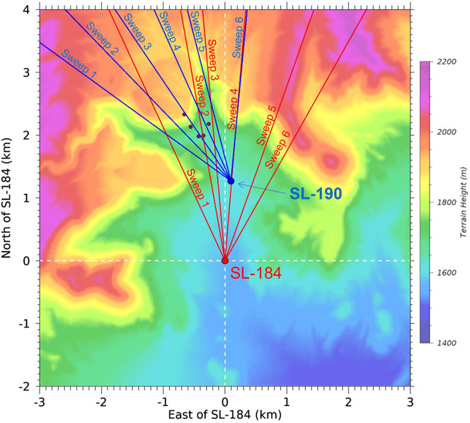
FIGURE 3. RHI scan directions used by SL190 (blue) and SL184 (red) during the smoke releases. For each lidar the scans are labeled “Sweeps” 1 through 6. Note that Sweep 4 from SL184 is coaligned with Sweep 6 from SL-190. Sweep 3 from SL190 was programmed to be aligned with the vertical smoke transect. The black dots indicate the Apron and Vertical Transect smoke locations.
Scanning lidars require additional careful calibration of the instrument’s heading direction because the scanning capability is used to accurately determine the lidar’s orientation. This is performed by directing the laser to “ping” off a nearby stationary target, such as a power pole. This calibration technique, when done carefully, allows for determination of the lidar’s heading direction to within ±0.1°. During post-processing the scanning lidars required a couple of error fixes. On occasion the time stamp in the datafiles “skipped” backwards in time by a few 100th of milliseconds. A correction was done to replace the erroneous time stamp with the average time computed from the two neighboring data rows. Secondly, a correction was made to correct for a long-term time drift that was seen partially in the data for SL190. This correction was necessary due to the inability of SL190’s computer to automatically sync with an external time-server and only affected a small portion of the data. A correction was done assuming a linear increase in time to correct the erroneous time stamps.
3.2.5 Sound detection and ranging (sodar)
Remotely sensed wind speed and direction measurements are also retrieved from the sodar near the Desert Rock Airport at NNSS (Figure 2A). This location is in an alluvial plain near the southern boundary of NNSS and ∼60 km from our study domain. Here, observations of the u, v, and w wind components are taken from 30 to 500 m, at 10 m height intervals, although often the maximum range gate with available data is closer to 250–300 m a.g.l. The sodar provided information about the wind profile at another NNSS location (for comparison) and at a higher temporal cadence (data are taken continuously) than the radiosonde launches and TBS missions. Sodar data are available as 15-minute averages.
3.2.6 Weather balloon and tethered balloon sensors
Profiles of Ta, RH, P, wind speed (U, m/s) and wind direction were collected using weather-balloon launched radiosondes (RS) and a tethered balloon system (TBS). Twenty-eight weather-balloon radiosondes (iMet-4, InterMet Systems, USA) were released during the METEX21 campaign, and their timing was done to coincide with each smoke release experiment. Nineteen of these flights were tracked to burst altitude (∼11 hPa, or about 30 km a.g.l.); the remaining others were either terminated early or telemetry was lost during the flight path. Note that wind speed and direction from the weather balloons is derived from the radiosonde’s GPS position. The radiosonde release point was 2 km south of the apron and co-located with the SL184, PL02, and MT08 (Figure 2B).
A TBS was deployed 400 m west of the radiosonde trailer (Figure 2B). This location proved to be somewhat problematic due to the presence of cross-valley canyon winds which increased shear and veer aloft for the 104 m3 aerostat tethered balloon and some flights were brought down prematurely for this reason. Enhanced winds and turbulence in this location also restricted flying the balloon all together on some smoke release days. Five TBS flights were conducted during METEX21 across four smoke experiment days (March 22, 24, 27, and 28). The tethered balloon was flown to a height of 400 m during the first flight on March 22nd and was moved up to 800 m on the next four flights. A flight altitude of 800 m above the valley aligns with an altitude of 450 m above the Aqueduct Mesa top. The TBS flew up to ten cup and wind vane anemometers for wind speed and direction, twelve iMet radiosondes (iMet XQ4 and iMet-4 RSB) for Ta, RH, P, and 3-d GPS, two Portable Optical Particle Sensors (POPS) (Handix Scientific, USA, Fan et al., 2020) for aerosol concentration and size distribution (0.14–3 micron range), and two condensation particle counters (CPC) for aerosol concentration (0.01–1 micron range). The POPS and CPC sensors were flown to capture any evidence of smoke plume transport across the balloon’s tethered path. The TBS also had a ground station for assessing wind gust (Ugust) and U as well as Ta, RH and P. All measurements were taken at 1 Hz.
3.2.7 Cameras
Scanning lidars, POPS, and CPC sensors were deployed to capture quantifiable evidence of the smoke plume. Qualitative information about plume behavior was captured using eight video cameras. The video cameras were placed in various locations to capture the smoke plumes from different angles and length scales. Some cameras were focused on the release points while other cameras had much wider angles and looked either down-valley or up-valley to capture longer-range transport behavior.
4 Results and discussion
4.1 Summary of flow and plume behavior
METEX21 collected more than 200 h of atmospheric observations to answer fundamental questions about flow in locally complex terrain and to provide validation data for atmospheric models. The variables U, direction, TKE, Ta, and L measured just above the valley floor (all but L were measured at MT08) are plotted in Figure 4 to show a time series of weather conditions during METEX21. Figure 4 also highlights the conditions observed during the smoke releases (time periods in gray boxes). Wind speed, direction and TKE varied greatly from day to day. Days with strong synoptic flow (March 21 and 26) saw moderate to strong northerly winds, enhanced daytime TKE, and cooler daytime temperatures. Days with locally driven flow (March 22, 27 and 28) experienced weaker daytime winds from the south and warmer daytime temperatures.
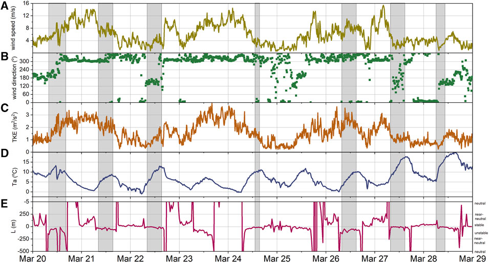
FIGURE 4. Time series of weather conditions in the METEX21 domain showing the 10 m (A) wind speed, (B) wind direction, (C) turbulence kinetic energy (TKE), and (D) air temperature (Ta) taken at MT08 in the P Tunnel Valley. The surface layer Obukhov length (L) is shown in panel (E). Note that L has been plotted only to ±500 (│L│> 500 is neutral stability) to show higher resolution during the other stability classes. Smoke release days and duration are highlighted in gray. Time is Pacific Standard Time.
We aimed to release smoke during different atmospheric stability conditions, although due to our daylight constraint for the smoke experiment, most of the transect releases were done either during near-neutral or unstable conditions (Figure 4E). The desert atmosphere transitions rapidly from stable to unstable as surface heating intensifies following sunrise. During METEX21, the Obukhov length values showed that the atmosphere was usually unstable (convectively well-mixed) by 0700 PST. Stable conditions developed again just after sunset around 1800 PST, but we did not capture this stability transition since our last smoke release was done at 1500 PST. One smoke release was done during strongly stable conditions, at 0600 PST (0700 PDT) on March 28, as seen in the time series of L in Figure 4E. In agreement with the Obukhov length, the TBS and weather balloon radiosondes also showed a lack of near-surface temperature inversion during most of our releases, indicating a well-mixed atmosphere. These diurnal observations of stability are consistent with March climatological averages of the Pasquill-Gifford stability parameter at NNSS (Soule, 2006).
Available energy in the METEX21 domain was partitioned mostly into the sensible heat flux, H (∼70%), followed by G and SG (∼20%) (not shown). Very little energy (<10%) was used for evapotranspiration. Given the low soil moisture levels (∼0.05 m3/m3) and limited amount of photosynthesizing vegetation, the very small LE fluxes are reasonable. Due to lack of both precipitation and extensive cloud cover during the experiment, the measured surface energy fluxes did not vary strongly from day to day. Small amounts of variability in the net radiation (Rn) flux, and the subsequent sensible heat (H) flux were due to the passing of occasional clouds in the afternoon hours.
Wind roses are shown for the three profiling lidars in Figure 5. The data were taken at 10 m (5a), 50 m (5b), and 100 m (5c) altitude and are shown for the hours overlapping with the tracer release days and times (0800-1500 PDT). The wind roses show dominant north-northwesterly winds, followed by a secondary dominance in south-southeasterly winds across the experiment domain and period. Northerly winds tended to be stronger than southerly winds and fastest on top of the Mesa (PL01). The stronger northerly wind speeds occurred during synoptically-driven wind events. On locally-forced days, the north-south valley flow reversal was a consistent feature for all measurement heights (10–150 m above the surface) in the valley based on PL02 and PL03. The 10 m tall met towers in the valley additionally show the same timing of the north-south flow reversal on non-synoptic forced days (as seen in Figure 4B at MT08).
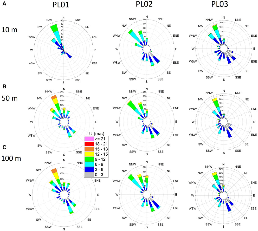
FIGURE 5. Wind roses at (A) 10 m, (B) 50 m, and (C) 100 m from the three profiling lidars during smoke release times only. Note that PL01 (4a) shows data from co-located MT01 because the Windcube v2 lidar has a minimum measurement of 40 m a.g.l.
While the met towers and lidars in the valley measured distinct along-axis valley flows in the METEX21 domain, the 2 m tall tripods measured much higher amounts of directional and velocity variability in the wind field (Figure 6) compared to the profiling lidars. The tripod towers also indicated the presence of slope flows along the mesa slope and edge, which are particularly visible in the data at Tripod 4, TT04. TT04 sees a wind pattern distinctly different from the others. This tower is located along the slope of Aqueduct Mesa and here the winds are channeled from the west from the nearby canyon and then forced upslope, resulting in a dominance of southwesterly winds. TT04 also sees upslope flows from the southeast, which are likewise observed on the apron at TT06. Note the observed anomalous wind direction at TT03. This tripod was placed on the eastern side of Aqueduct Mesa in a shallow dip in topography and that location appears to see very light winds from the west in that depression. The actual smoke release location (M03) was closer to the mesa edge (Figure 2C).
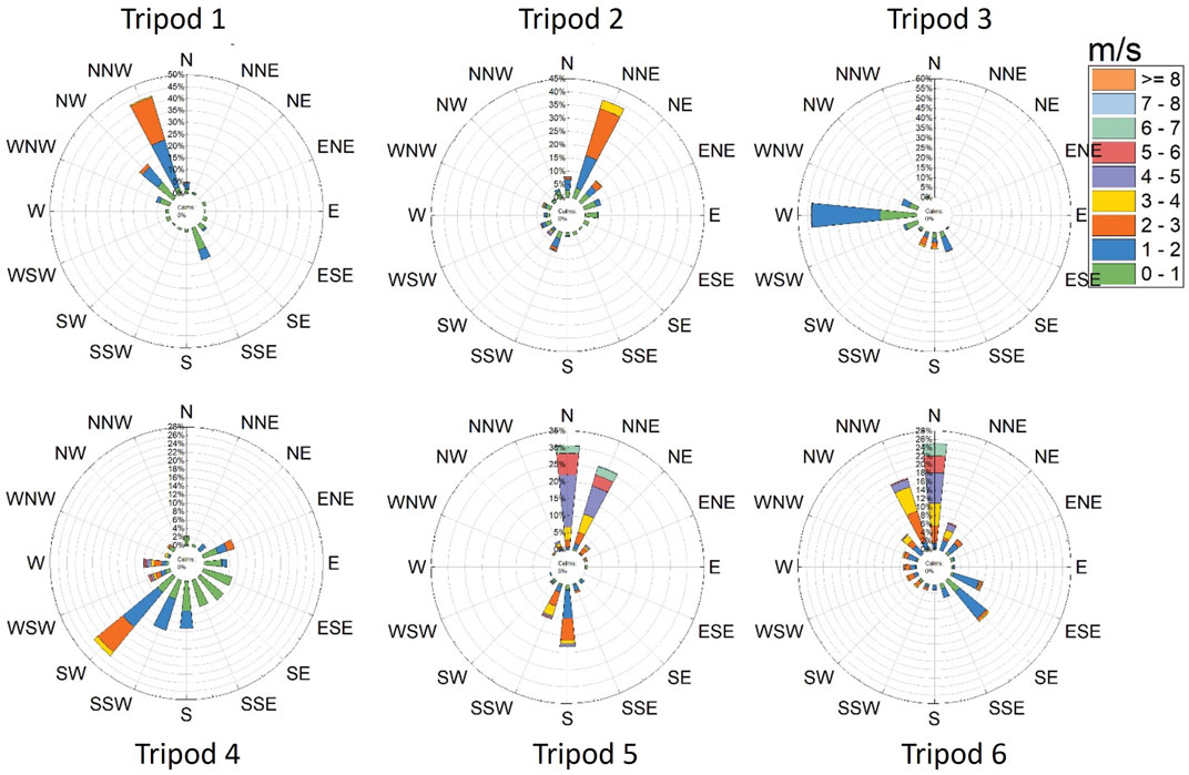
FIGURE 6. Wind roses of the 2 m height winds observed during smoke release times only. The data show very high spatial variability just above the ground and at these locations. Tripods 1–3 are on the Mesa edge (smoke release points M01–M03), Tripod 4 is on the Mesa slope (smoke release point M04), and Tripods 5 and 6 are on the P tunnel apron (at smoke release points A01 and A02).
Still images from video also showed evidence of slope and valley flows. Figure 7 shows two smoke release experiments planned 2 hours apart on March 28. The first release at 0600 PST/0700 PDT (Apron Transect Release) shows smoke transported down-valley from the apron (Figure 7A) as it stays close to the ground surface under weak north-to-south drainage winds (measured by the valley met towers, Figure 4B, and PL02 and PL03) and a strongly stable atmosphere (measured by the Blackbrush flux tower, Figure 4E). By 0800 PST/0900 PDT local heating in the valley has already created enough buoyant mixing to erode the stable boundary layer (Figure 4E) and the smoke plumes during this release (Vertical Transect Release) are transported immediately upslope (following the mesa and ridgelines that border the P-tunnel apron, Figure 7B), even though the dominant winds over the valley have shifted to the southerly direction and are flowing up-valley (Figure 4B).
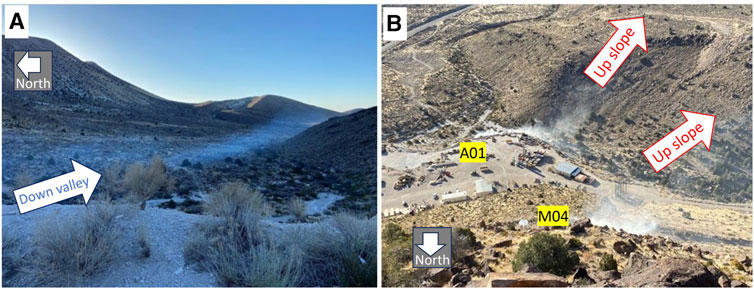
FIGURE 7. Photographs showing evidence of the smoke plume being transported (A) down-valley (A) and with (B) upslope flow. These photographs were taken on March 28 around 0700 PDT and 0900 PDT, respectively. In (A) the release points were on the apron (an Apron Transect release). In (B) the visible release points are A01 and M04 (a Vertical Transect release). Photograph (A) was taken from the edge of the apron looking southeast down the P-tunnel valley; photograph (B) was taken from the top of Aqueduct Mesa.
The cameras captured the finer features of the smoke behavior well, but the visible smoke was only detectable to the eye out to 1 km (during our single stable release time) and usually out to much shorter distances from the release points during most of the releases due to well-mixed conditions. The SLs and TBS were deployed farther down-valley to detect the plumes beyond the camera footage. The SLs using RHI scans proved extremely effective in measuring and detecting the smoke plume (via the attenuated backscatter coefficient) at distances out to 2–3 km from the release points. These scanning lidar plume detection results are presented in detail for the two case study days.
While we aimed to deploy four particle counters on the TBS to validate plume transport, the two CPCs proved to be problematic and were not flown on every mission meaning that TBS flights later in the campaign flew only two aerosol sensors (POPs) – mostly at altitudes of 80 m and 300 m. A likely plume detect, i.e., significant increase in particle number concentration in the expected particle size range, was detected on the 80 m level POPs on March 28, and with more uncertainty at various altitudes on March 22. On March 28 we saw an increase in number concentration and mean particle diameter corresponding with the first Apron release of the day (Figure 7A). Further details about the possible March 22 detects are discussed in the Case Days below.
4.2 Case days
4.2.1 Synoptically-forced flow over NNSS
A set of four simultaneous Apron and Vertical Transect releases were done on March 21. Each smoke release lasted 30-minutes. Start times were 1500, 1700, 2000, and 2200 UTC (0800, 1000, 1300, and 1500 PDT). Because two transects were lit simultaneously a total of five smoke release locations (M02, M04, A01, A02, A03) were used during all releases on this day. A single radiosonde was launched 10 minutes after the start of each smoke release for a total of four radiosonde releases. Due to some last-minute logistical issues and high wind speeds, the TBS was not in operation.
Wind observations from the meteorological towers, profiling lidars, sodar, and weather balloon radiosondes showed evidence of strong synoptically-driven flow throughout the entire day and winds were from the north or north-northwest at all release times and locations. The 10 m wind speeds averaged 10–12 m/s over the Aqueduct Mesa, 6–10 m/s over the P-tunnel valley, and 5–6 m/s over the north end of Yucca Flat during these smoke releases. PL01-03 showed little shear and veer in the wind profiles (up to 150 m a.g.l.) over the Mesa and valley as well. Figure 8 highlights the near-surface wind speeds and directions measured by the MT and TT anemometers near the release points and at the four start times. Although there is some variability in wind speed in this plot, the direction is largely from the north showing that dominant synoptic flow was seen even a few meters off the ground at most locations near the apron and on the Mesa where the terrain is most complex. One exception was Met Tower 4 on the Mesa slope (M04 smoke release point) which saw local flow channeled down the canyon from the west or southwest due to that local terrain feature.
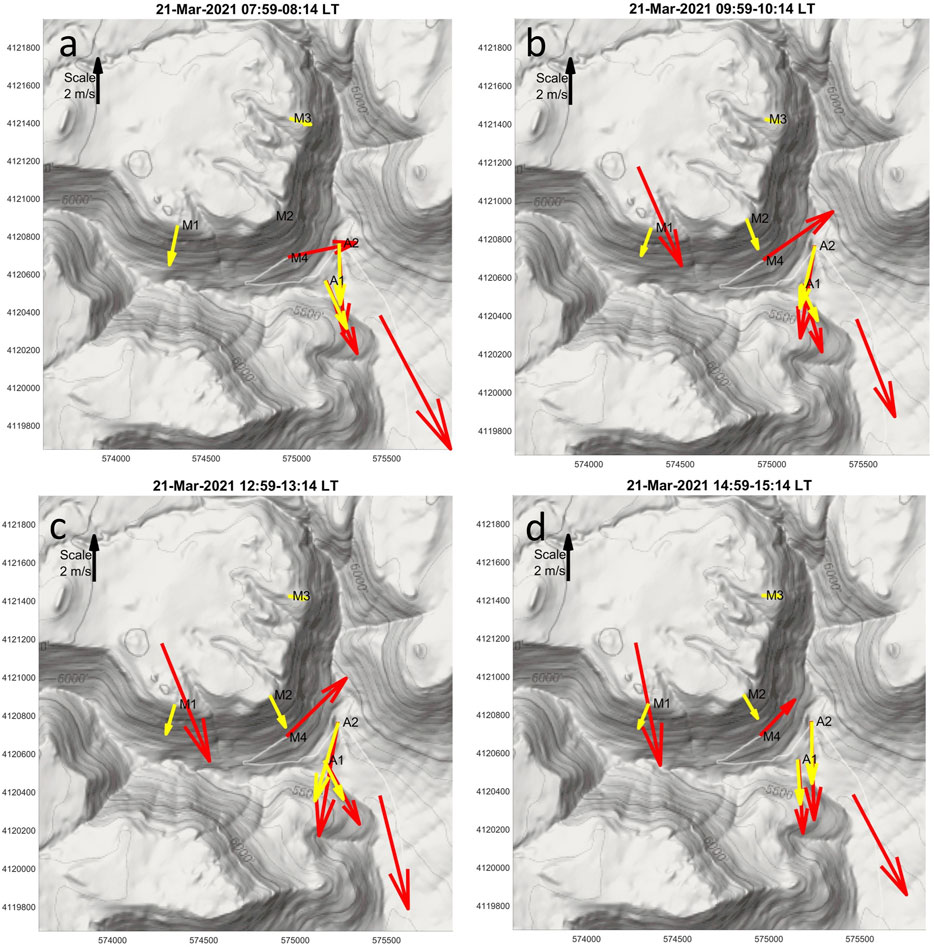
FIGURE 8. 15-minute average near-surface winds at the tripod towers and meteorological towers, including those locations co-located with the smoke releases at M1, M2, M3, M4, A1, and A2 on March 21. Average wind conditions during the first 15 minutes of each release time are shown here (A–D). Red vectors are the 10 m MT winds, yellow vectors are the 2 m TT winds. The black arrow shows the velocity scale and direction of north.
The four radiosondes launched showed north winds (not shown) within the first couple of kilometers of the PBL which turn westerly above 5 km. Westerlies at high altitude are consistent with the climatological record of radiosonde-derived wind directions found aloft at NNSS. The stability data (radiosonde temperature profiles; Obukhov length, Figure 4E) indicated a weakly unstable atmosphere during the day’s smoke releases.
RHI measurements are shown in Figures 9, 10 for the second release of the day, a 1000 local time (1700 UTC) Apron and Vertical Transect release. Focusing on the closest SL first, SL190, we see strong negative radial velocities (i.e., indicating flow towards the lidar) in nearly all of the sweeps, indicating that the winds are from the north-northwest over the Mesa and over the valley. Data availability from the scanning lidar is much sparser over the Aqueduct Mesa (Sweeps 2–4 in Figure 9), however MT01 and PL01 confirm northerly winds over the Mesa. Sweep 3’s line of sight goes directly over the apron smoke release points and the Aqueduct Mesa. This sweep (9c) as well as Sweep 2 (9b) also indicates some weak upslope flow behavior (positive radial velocities) on the leeward (south-facing) side of Aqueduct Mesa. This could be due to a roll vortex or weak recirculation eddy that formed in the wake of the Mesa and extends 200 m downwards from the top of the Mesa to the apron surface.
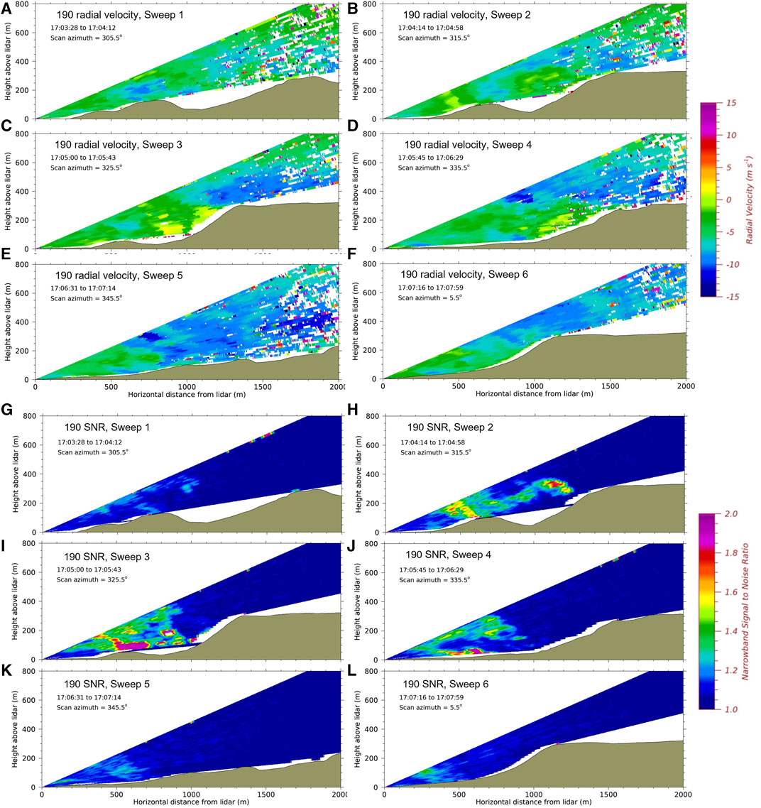
FIGURE 9. (A–F) Sequence of RHI scans with changing azimuth angle showing radial velocity as observed by SL190 during the smoke release at 1700 UTC (1000 PDT) on 21 March. (G–L) Sequence of RHI scans showing SNR as observed by SL190 during the same smoke release. Sweep numbers correspond with the scans in Figure 3. Data impacted by terrain have been masked out.
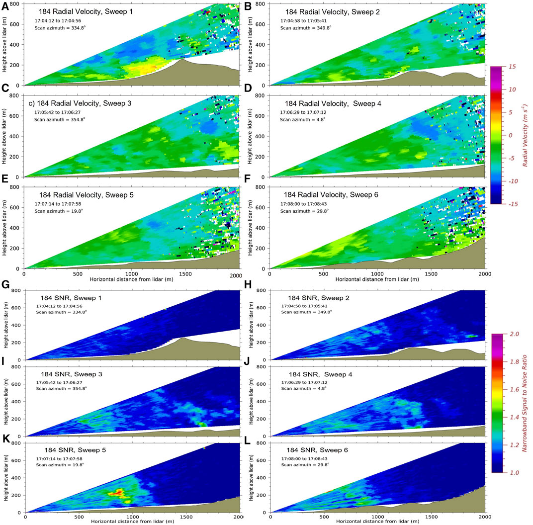
FIGURE 10. Same as Figure 9, except for SL184.
There is smoke visible in all the sweeps in this sequence, although Sweeps 2 through 4 show the highest smoke concentrations (Figures 9H–J). In Sweep 2, there is clearly a smoke plume coming from the Mesa top (release point M02) and being transported over the recirculation eddy and is then mixed down at the north end of the valley. Sweeps 4–6 show the combined smoke plumes traveling down the valley, consistent with the dominant northerly wind direction. These images indicate that SL190 is able to distinguish the smoke release point on the mesa edge from those plumes originating from the apron 270 m below. But it does not appear to distinguish the horizontally separated smoke release points on the apron (separated by a ground distance of 300 m).
Lidar results for SL184, deployed down-valley of SL190 and farther from the release sites, are shown in Figure 10. This lidar also measured negative radial velocities in the P-tunnel valley indicating northerly flow farther away from the apron. Sweep 1 shows some weak upslope flow behavior on the leeward side of a ridge just south of Aqueduct Mesa. Although the lidar did not have good line of sight past this southerly ridge to release points A01 and A03 on the apron, we did observe highly variable smoke behavior in the video footage indicating that another roll vortex may have been present between the south ridge and the P tunnel apron (e.g., in the lee of Aqueduct Mesa). A 3d sonic tripod was not installed at A03, however the tripod at A02 did show highly variable wind direction data during this 30-min release time.
There is no evidence of the plume in the leeward south ridge recirculation feature captured in Sweep 1 (Figure 10G), but a smoke plume likely coming from the apron, ∼2 km from the lidar, is visible in Sweep 3 (Figure 10I). It is clear from this sequence of scans that the smoke is more dispersed as it travels down the valley; the back scatter signal is much weaker at the southern end of the valley (and closer to the lidar) than it was at the very north end near the apron. In this RHI scan sequence, the strongest backscatter is observed in Sweep 5 (Figure 10K) when the plume is transported down the valley and the highest concentration signal occurs at this time approximately 250 m above the valley floor (800–900 m ground distance from the lidar). SL184 also shows that the plume is detectable at altitudes up to 400 m a.g.l. above the valley floor as it moves southward. The plume may continue to vertically disperse and extend up to higher altitudes as it moves southward and towards Yucca Flat, but those altitudes were outside the range of the lidar.
4.2.2 Locally-forced flow over the 5-km domain
A set of mesa edge releases (M01, M02, and M03) were conducted at 1530, 1700, 2000, and 2200 UTC (0830, 1000, 1300 and 1500 PDT) on March 22. A single radiosonde was launched 10 minutes after the start of each smoke release for a total of four radiosonde releases. The TBS was flown during the first three releases. It was brought down after release #2 and re-flown for release #3.
The network of wind sensors (towers, lidars, TBS) across the 5-km domain captured higher spatial variability in wind behavior on March 22 than the previous case study day. This was caused by the lack of strong synoptic forcing over the valley and the presence of thermally-driven upslope and up-valley flows at the release times, which can be in different cardinal directions depending on location. The wind vectors based on the 2 m tripods and 10 m met towers are shown in Figure 11 for times around the second release of the day (1000 PDT). Up-valley flow (from south-to-north) was detected by the tripods and met towers on the apron and at the northern end of the P tunnel valley. Upslope flow was detected on the Mesa slope (M4). On occasion, upslope flows were also detected on the top of Aqueduct Mesa and reached as far as 600 m from the mesa edge. Otherwise, winds above the top of Aqueduct Mesa (at PL01 and MT01) largely came from the north, showing a decoupling between flow found over the Mesa (northerly) and flow observed just above the valley floor and on the apron (southerly).
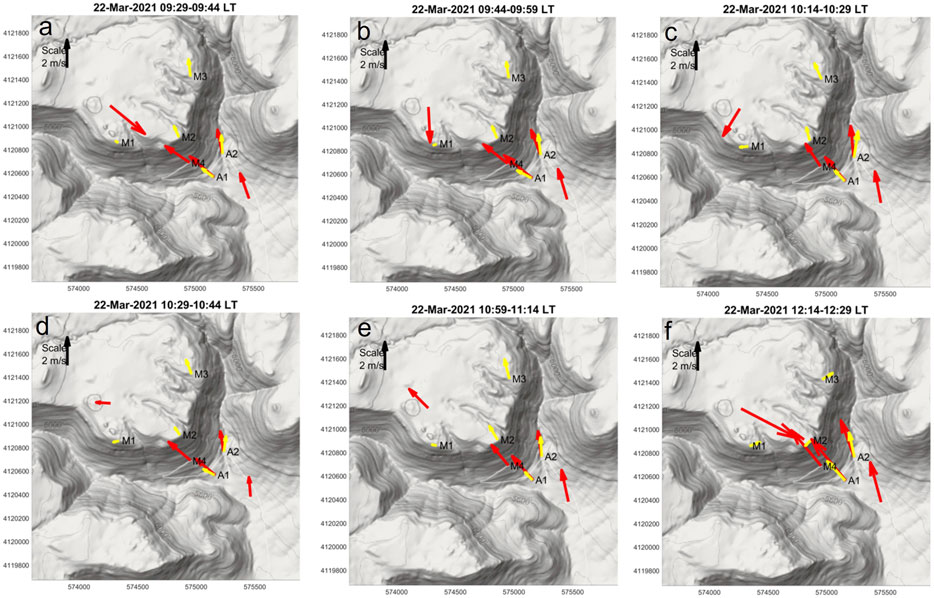
FIGURE 11. 15-minute average wind vectors shown for times around the second smoke release (1000 PDT) on March 22. (A–F) highlight the amount of wind variability seen from ∼0930 to ∼1230 PDT (local time). On this day smoke was released from the three locations along the Mesa edge (M1, M2 and M3). Red vectors are the 10 m tall towers (MT); yellow are the 2 m tall tripods (TT). The black arrow shows the velocity scale and direction of north.
A veer layer shows up distinctly in the radiosonde and TBS measurements. While all daytime winds below ∼400 m a.g.l. over the valley were from the south (verified by the radiosonde and TBS, as well as PL02, PL03 and MT02-11 (MT08 is shown in Figure 4B)), northerly flow was observed in the winds aloft. The radiosonde showed a distinct wind direction shift to the north occurring between 400 and 500 m, while wind direction at the TBS just above 400 m clearly shows northerly flow as well (Figure 12A). Note that because the radiosonde is moving with the wind, the locations are no longer co-located once the radiosonde balloon is released. When the TBS was brought down around 1800 UTC (1100 PDT) due to wind gusts aloft, the anemometers showed an abrupt wind direction shift slightly lower around 320 m (Figure 12A). This suggests that flow at least in the first couple hundred of meters over the valley and apron was locally-driven by strong diurnal heating, while winds at the higher altitudes (>400 or 500 m) and elevations were mostly from the north during the first two smoke releases. Data availability from the sodar, deployed at the southern end of NNSS, is unfortunately patchy above 300 m a.g.l. making it difficult to assess the regional extent of this veer layer.
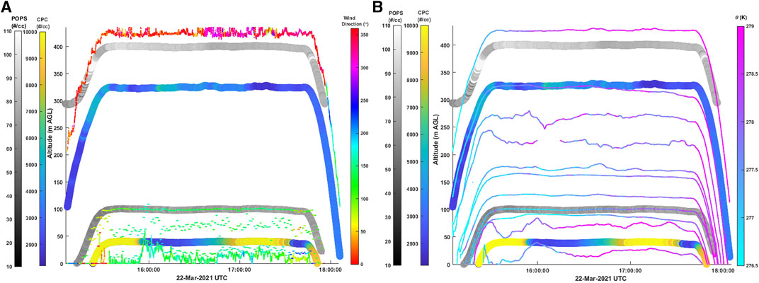
FIGURE 12. Time series of TBS (A) wind direction and (B) potential temperature. The panels also show a time series for the POPS (100 m and 400 m) and CPC (40 m and 325 m) total number particle concentration during the first two smoke releases on March 22. Tethered balloon observations shown here include 1505–1805 UTC, or 0745-1105 local time. Note that the TBS was brought down at 1745 UTC due to high wind shear and redeployed a few hours later.
Temperature sensors were flown at altitudes from 20 to 400 m a.g.l. on March 22. The potential temperature gradient indicated well mixed conditions during the releases (the first two releases are shown in Figure 12B). This is largely in agreement with the surface flux tower stability parameter, L, measured farther down the valley. Four aerosol sensors were also flown at ∼40, 100, 320 and 400 m a.g.l. On this day the smoke releases were conducted on the Mesa edge at an average elevation of 1920 m a.s.l., or 350 m above the average valley floor. Note that this altitude is roughly equivalent to the heights of the 400 m POPS sensor and 300 m CPC sensor. There is a small increase in particle count at the 400 m POPS after the first release (1530 UTC) (Figure 12). This may be an indication that the plume was transported from the top of the Mesa down to the valley by northerly winds at this altitude, although the small increase makes a definite “hit” hard to determine. A small increase at the 300 m CPC around 1620 UTC and a larger increase at the 50 m CPC sensor at 1530–1600 and 1700–1740 UTC are also seen. These may indicate that the plume has been transported by higher altitude northerly winds and then mixed down into the valley at the TBS location.
Plume detection was more definitively made by the scanning lidars, and the profiling lidar (PL01) on top of Aqueduct Mesa. Figures 13A–F shows the radial velocities measured during the second release (1700 UTC) at SL190, where positive velocities indicate winds flowing away from the lidar, or up-valley and/or upslope on Aqueduct Mesa. Sweeps 2–4 scanned directly over the apron and Aqueduct Mesa. These scans show up-valley winds over the apron and northern end of the P tunnel apron. They also show strong upslope flows on Aqueduct Mesa which extend up to ∼200 m in altitude at this time step (Figures 13B–D). Above this altitude the radial velocities are negative and indicate flow from the north on top of the Mesa. SL190 data showed that the plumes were transported immediately to the south of the mesa edge (driven by northerly winds above the mesa) but are soon lifted vertically due to the converging surface flows, and are transported back to the north by the presence of these upslope winds. This caused the smoke to be visible in the scanning lidar data over the Mesa top to a horizontal distance of at least 300 m from the Mesa edge (Figures 13I,J). The profiling lidar backscatter data from PL01, placed 600 m from the Mesa edge, also showed a 10-minute-long significant spike in carrier-to-noise ratio at altitudes of 40–130 m a.g.l. at this time (1030–1040 PDT (1730–1740 UTC)) that is significantly above the ambient CNR for all other times. At other times during weaker upslope flows, it appears that the smoke is transported down-valley instead of being lifted over the Mesa.
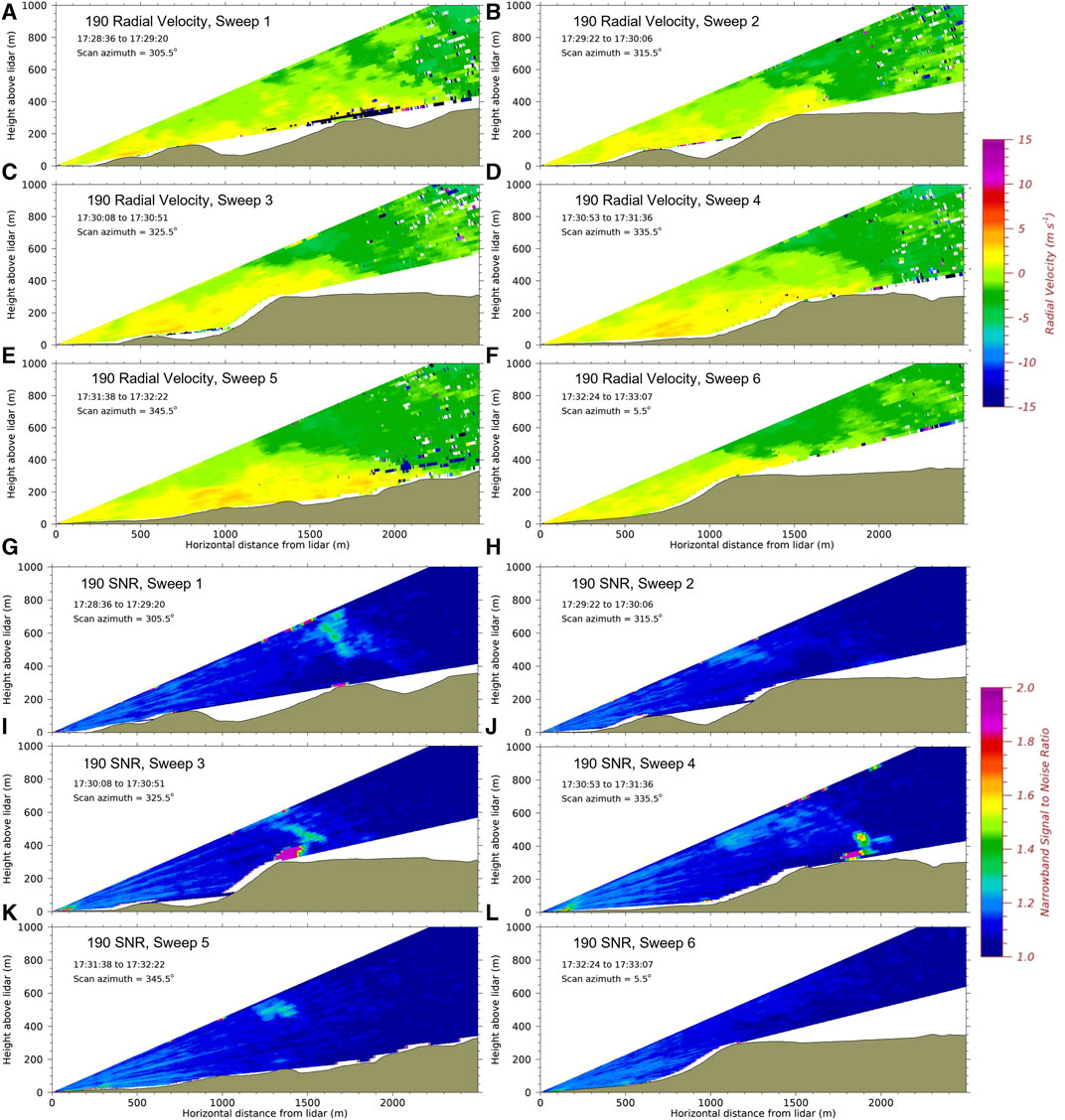
FIGURE 13. (A–F) Sequence of RHI scans showing radial velocity as observed by SL190 during the second smoke release on 22 March. (G–L) Sequence of RHI scans showing SNR as observed by SL190 during the same smoke release. Sweep numbers correspond with the scans in Figure 3.
SL184 is roughly co-located with the TBS and provides additional insight into plume transport farther down the valley. This lidar shows evidence of up-valley flow (i.e., winds flowing away from the lidar) up to altitudes of 200–400 m above the valley floor, depending on location, while northerly winds are found at higher altitudes and elevations (Figures 14A–F). There is evidence that the plume from the 1700 UTC release has reached SL184 (a distance of 2 km from the smoke release points). The lidar recorded smoke around 1730 UTC in Sweeps 4–6 (Figures 14J–L) suggesting that the enhanced aerosol count on the TBS’s 50 m CPC sensor from 1700 to 1740 UTC is likely showing the smoke plume. For the plume to travel down-valley while the winds were largely up-valley, it is likely that the plume, originating from the Mesa edge, was transported first by northerly winds aloft, and then mixed downward into the air space over the valley; first by entrainment, and then brought closer to the surface due to strong buoyant mixing or downward motions near surface associated with divergence. This scenario is also supported by SL184 which shows the smoke plume being transported at high altitudes as it moves down the valley.
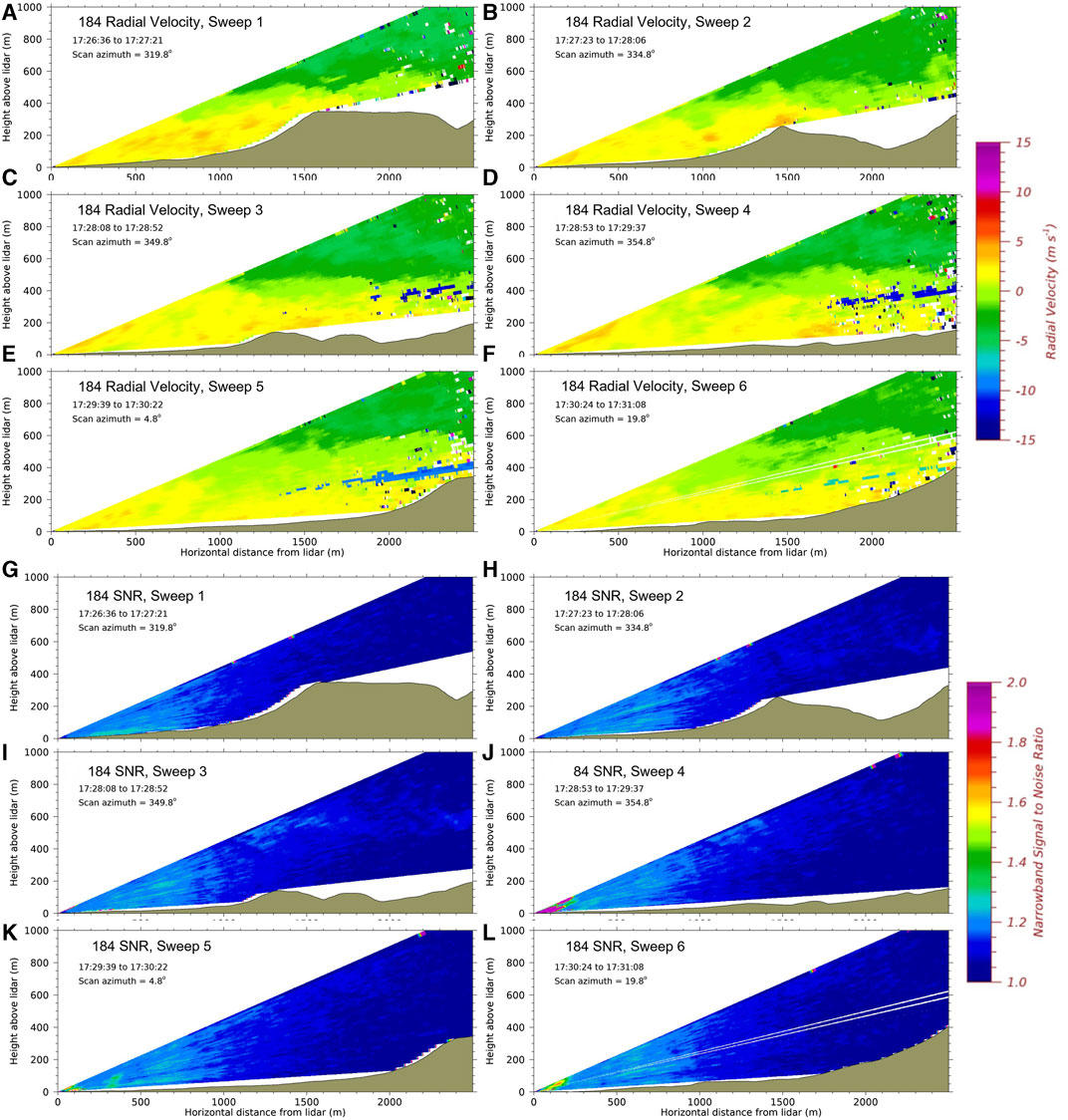
FIGURE 14. Same as Figure 13, except for SL184.
5 Conclusion
Lidar have been used previously to detect the presence of aerosols, although most studies show their use for tracking ambient particulate matter for air-quality studies. For example, in the French Alps ground-based Raman lidar and aircraft lidar were used to sample aerosol, water vapor and temperature profiles in an area subject to valley and mountain winds (Chazette and Totems, 2023). While ground-based Raman lidar allowed the study of the vertical distribution of aerosols, we showed during METEX21 that ground-based Doppler scanning lidar can also provide information about aerosol concentration in the 2-d. We showed the use of Doppler lidar for tracking experimental smoke plumes in continuous time and out to long-range distances (out to 2–3 km) as they were transported and dispersed both in the vertical and horizontal directions by the ambient atmosphere environment. The scanning lidars proved more effective at tracking the plume transport than did the single, stationary TBS or video cameras.
Our plume observations indicate less predictable plume behavior during locally-driven conditions than on synoptic weather days. This has implications for planning future tracer release experiments at NNSS where the aim is to measure dual tracers down-valley of the P tunnel apron. We also showed how elevation and altitude affects plume transport by executing releases on the mesa top and apron below. The scanning lidars were able to distinguish the release locations separated by the 300 m elevation but had a harder time distinguishing horizontally displaced distances. The full array of different instruments and sensor platforms also showed the complexity of flow in locally complex terrain and how this influences the dispersion and transport of tracers. Lastly, our observations show the need for collecting data in the vertical direction as well as the horizontal, as shear and veer, induced by terrain features, played a large role in determining plume behavior. Future campaigns will include multiple TBSs including additional temperature profiling and aerosol counter instrumentation as this set of observations was deemed insufficient across our domain during METEX21.
Data availability statement
The raw data supporting the conclusion of this article will be made available by the authors, without undue reservation.
Author contributions
All authors listed have made a substantial, direct, and intellectual contribution to the work and approved it for publication.
Funding
This research was funded by the National Nuclear Security Administration, Defense Nuclear Nonproliferation Research and Development (NNSA DNN R&D) Office.
Acknowledgments
This experiment was part of the Low Yield Nuclear Monitoring (LYNM) program and funded by the National Nuclear Security Administration, Defense Nuclear Nonproliferation Research and Development (NNSA DNN R&D). The work was partially performed under the auspices of the U.S. Department of Energy by Lawrence Livermore National Laboratory under Contract DE-AC52-07NA27344. The authors acknowledge important interdisciplinary collaboration with scientists and engineers from ARL/SORD, LANL, LLNL, MSTS, PNNL, and SNL. Special thanks go to those who helped collect field data, including, but not limited to, Ethan Alger (Experiment Lead), Wayne Bailey, Art Bockman, Duli Chand, Patrick Conry, Beth Dzenitis (Experiment Lead), Rick Lantrip, Casey Longbottom, Kale McLin, Michael Moore, Matt Nelson, Bob White, and Lynn Wood (Experiment Lead), and scientific input from Steve Myers, Michael Foxe, Cari Seifert, and Lee Glascoe. Additionally, we’d like to thank the operators and workers at the P tunnel complex for their assistance and willingness to accommodate our field schedule. Internal publication number, LLNL-JRNL-850942.
Conflict of interest
The authors declare that the research was conducted in the absence of any commercial or financial relationships that could be construed as a potential conflict of interest.
Publisher’s note
All claims expressed in this article are solely those of the authors and do not necessarily represent those of their affiliated organizations, or those of the publisher, the editors and the reviewers. Any product that may be evaluated in this article, or claim that may be made by its manufacturer, is not guaranteed or endorsed by the publisher.
References
Allwine, J., and Flaherty, J. (2006). Joint Urban 2003: study overview and instrument locations. Pacific Northwest National Laboratory, 92. Tech. Rep. PNNL-15967.
Baldocchi, D. D. (2003). Assessing the eddy covariance technique for evaluating carbon dioxide exchange rates of ecosystems: past, present and future. Glob. Change Biol. 9, 479–492. doi:10.1046/j.1365-2486.2003.00629.x
Banta, R. M., Olivier, L. D., Gudiksen, P. H., and Lange, R. (1996). Implications of small-scale flow features to modeling dispersion over complex terrain. J Appl. Meteorology Climatol. 35 (3), 330–342. doi:10.1175/1520-0450(1996)035<0330:iossff>2.0.co;2
Chazette, P., and Totems, J. (2023). Lidar profiling of aerosol vertical distribution in the urbanized French alpine valley of Annecy and impact of a Saharan dust transport event. Remote Sens. 15 (4), 1070. doi:10.3390/rs15041070
Fan, M., McMeeking, G., Pekour, M., Gao, R.-S., Kulkarni, G., China, S., et al. (2020). Performance assessment of portable optical particle spectrometer (POPS). Sensors 20 (21), 6294. doi:10.3390/s20216294
Fiedler, F., and Borrell, P.TRACT (2000). “Transport of air pollutants over complex terrain,” in Exchange and transport of air pollutants over complex terrain and the sea (Germany; New York, NY, USA: Springer-Verlag: Berli/Heidelberg), 223–268. 3-540-67438-1.
Martin, D., Nickless, G., Price, C. S., Britter, R. E., Neophytou, M. K., Cheng, H., et al. (2010). Urban tracer dispersion experiment in London (DAPPLE) 2003: field study and comparison with empirical prediction. Atmos. Sci. Lett. 11, 241–248. doi:10.1002/asl.282
Mauder, M., Foken, T., and Cuxart, J. (2020). Surface-energy-balance closure over land: a review. Boundary-Layer Meteorol. 177, 395–426. doi:10.1007/s10546-020-00529-6
Nasstrom, J. S., Sugiyama, G., Baskett, R. L., Larsen, S. C., and Bradley, M. M. (2007). The National Atmospheric Release Advisory Center modelling and decision-support system for radiological and nuclear emergency preparedness and response. Int. J. Emerg. Manag. 4, 524–550. doi:10.1504/ijem.2007.014301
Orgill, M. M., and Schreck, R. I. (1985). An overview of the ASCOT multi-laboratory field experiments in relation to drainage winds and ambient flow. Bull. Am. Meteorological Soc. 66, 1263–1277. doi:10.1175/1520-0477(1985)066<1263:aootam>2.0.co;2
Panofsky, H. A., and Dutton, J. A. (1984). Atmospheric turbulence – models and methods for engineering applications. New York: John Wiley & Sons, 397.
Parrish, D. D., Allen, D. T., Bates, T. S., Estes, M., Fehsenfeld, F. C., Feingold, G., et al. (2009). Overview of the second Texas air quality study (TexAQS II) and the gulf of Mexico atmospheric composition and climate study (GoMACCS. ). J. Geophys. Res. – Atmos. 114, D00F13. doi:10.1029/2009JD011842
Poulos, G. S., and Bossert, J. E. (1995). An observational and prognostic numerical investigation of complex terrain dispersion. J Appl. Meteorology Climatol. 34 (3), 650–669. doi:10.1175/1520-0450(1995)034<0650:aoapni>2.0.co;2
Soule, D. A. (2006). Climatology of the Nevada test site. SORD Technical Memorandum SORD 2006-03, 171.
Stull, R. B. (1988). An introduction to boundary layer meteorology. Dordrecht: Kluwer Academic Publishers, 670.
Thullier, R. H. (1992). Evaluation of a puff dispersion model in complex terrain. J. Air Waste Manag. Assoc. 42, 290–297. doi:10.1080/10473289.1992.10466992
Wharton, S., Newman, J. F., Qualley, G., and Miller, W. O. (2015). Measuring turbine inflow with vertically-profiling lidar in complex terrain. J. Wind Eng. Industrial Aerodynamics 142, 217–231. doi:10.1016/j.jweia.2015.03.023
Wiersema, D. J., Wharton, S., Arthur, R. S., Juliano, T. W., Lundquist, K. A., Glascoe, L. G., et al. (2023). Assessing turbulence and mixing parameterizations in the gray-zone of multiscale simulations over mountainous terrain during the METEX21 experiment. Front. Earth Sci. 11. doi:10.3389/feart.2023.1251180
Keywords: atmospheric transport and diffusion, tracers, anabatic and katabatic flow, valley flows, LIDAR-remote sensing, field campaign observations, complex terrain
Citation: Wharton S, Brown MJ, Dexheimer D, Fast JD, Newsom RK, Schalk WW and Wiersema DJ (2023) Capturing plume behavior in complex terrain: an overview of the Nevada National Security Site Meteorological Experiment (METEX21). Front. Earth Sci. 11:1251153. doi: 10.3389/feart.2023.1251153
Received: 30 June 2023; Accepted: 23 October 2023;
Published: 23 November 2023.
Edited by:
Kevin Cheung, E3-Complexity Consultant, AustraliaReviewed by:
Manuela Lehner, University of Innsbruck, AustriaYubin Li, Nanjing University of Information Science and Technology, China
Copyright © 2023 Wharton, Brown, Dexheimer, Fast, Newsom, Schalk and Wiersema. This is an open-access article distributed under the terms of the Creative Commons Attribution License (CC BY). The use, distribution or reproduction in other forums is permitted, provided the original author(s) and the copyright owner(s) are credited and that the original publication in this journal is cited, in accordance with accepted academic practice. No use, distribution or reproduction is permitted which does not comply with these terms.
*Correspondence: Sonia Wharton, d2hhcnRvbjRAbGxubC5nb3Y=