Near-field variability of evaposublimation in a montane conifer forest

Methods that combine in-situ measurements, statistical methods, and model simulations with remotely sensed data provide a pathway for improving the robustness of surface flux products. For this research, we acquired eddy-covariance fluxes along a five-tower transect in a snowy montane forest over three consecutive winters to characterize near-field variability of the subcanopy environment. The novel experiment design enabled discriminating near-field evaposublimation sources. Boosted regression trees reveal that the predictive capacity of state variables change with season and storm cycle frequency. High rates of post-storm evaposublimation of canopy-intercepted snow at this site were constrained by short residence time of snow in the canopy due to throughfall and melt. The snow melt-out date for open vs. closed canopy conditions depended on total snowfall accumulation. Compared with low accumulation years, the snow melt-out date under the dense canopy during the high accumulation winter was later than for the open area, as shading became more important later in the season. The field experiments informed an environmental response function that was used to integrate ERA5-Land latent heat flux data at 20-km nominal resolution with USFS Tree Canopy Fraction data at 30-m resolution and showed near-field flux variability that was not resolved in model simulations. Previous evaposublimation results from experiments in alpine and subalpine environments do not directly translate to a montane forest due to differences in process rates.

1 Introduction

Montane forests are a dominant land cover type in the Sierra Nevada range of the western United States (Barbour et al., 1991). Processes that govern snow accumulation and ablation in montane forests are therefore critical for understanding the water cycle, monitoring forest health and forecasting spring runoff (Heckmann et al., 2008; Kirchner et al., 2020; Krogh et al., 2022). Evaposublimation—the combination of evaporation and sublimation—is an important ablation process in a montane environment, where wintertime air temperatures vacillate around freezing. Due to heterogeneity in canopy height, canopy gaps, aspect and other topographic and forest structure parameters, quantifying evaposublimation challenges both technical assumptions and measurement capabilities (Svoma, 2016; Conway et al., 2018). Forests present significant difficulties for compiling important snow parameters needed to initialize snowpack models (Rutter et al., 2009; Kim et al., 2021). Due to hypsometry of the Sierra Nevada and many other mountain ranges, montane forest ecosystems have greater areal extent than alpine or subalpine climate zones. Despite this relative spatial importance of montane forests for hydrology and net ecosystem exchange, the processes that drive evaposublimation in montane forests remain poorly constrained.

One approach to directly measure evaposublimation rates in forested environments has been to deploy an eddy-covariance (EC) system on a tower in a basin of interest. The EC system is mounted sufficiently high that heterogeneous sources from below are blended to yield a flux representative of a large measurement footprint (the upwind area over which the flux is integrated) yet not so high that significant storage below the measurement height occurs (Foken, 2008). However, attributing EC-derived fluxes to a particular forest structure presents additional challenges. For example, in montane environments, thermodynamically stable meteorological conditions near the surface can reduce mixing and generate drainage flows and may frustrate even carefully considered deployments. Also, above-canopy sensible and latent heat fluxes may not be representative of the subcanopy environmental state (Thomas and Foken, 2007; Drake et al., 2022). More pointedly, an integrated measurement of evaposublimation over the tower footprint may be helpful for operational estimation of winter water loss from a particular catchment but it provides little actionable information for improved understanding of the contribution by forest heterogeneities to evaposublimation processes.

A promising field-based technique for assessing the role of forest heterogeneity for fluxes over larger scales has been to develop environmental response functions from airborne (Metzger et al., 2013) and tower-based EC measurements (Xu et al., 2017). This method utilizes a wavelet technique to discretize turbulence and thereby produce fluxes as a function of length scale. Direct attribution of fluxes derived by this method to particular landscape features is challenging because of an asymmetrical response of fluxes between smooth-to-rough and rough-to-smooth transitions in surface roughness characteristics (Albertson and Parlange, 1999). Despite potential ambiguity in associating landscape features with fluxes, the use of environmental response functions in Metzger et al., 2013; Xu et al., 2017 aligns with the goal of deriving fluxes from instruments on satellite-based platforms. Currently, evaposublimation cannot be measured directly by remote sensing techniques so auxiliary sources must be integrated with remotely sensed data to infer fluxes.

Physical models initialized with spaceborne and other measurements have been implemented to produce flux estimates over subalpine forests. For example, Snowpack/Alpine-3D and Snowmodel have been employed to estimate spatiotemporal distribution of sensible and latent heat flux (e.g., Lehning et al., 2004; Liston and Elder, 2006). However, these models (and others) rely upon Monin-Obukhov Similarity Theory (MOST) to estimate wind-related parameters such as speed, friction velocity, and aerodynamic roughness for calculating fluxes above the canopy. Lacking a practical alternative, MOST has been implemented in models to estimate fluxes even though assumptions of horizontal terrain, turbulence homogeneity and stationarity are routinely violated. An additional deficiency of model-derived fluxes is that the model resolution may be too coarse to accurately represent the environmental response of vegetation to estimated fluxes. Fluxes from the subcanopy environment are difficult to partition from above canopy fluxes. Subcanopy fluxes are key drivers of the thermodynamic state characterizing near-snow-surface humidity and temperature and hence, are critical to understanding ablation processes and the aridity state of the subcanopy environment. Alternative methods are needed to assess and improve upon the robustness of fluxes derived in forested areas by MOST and remote sensing.

The purpose of this research is to examine how subcanopy sensible and latent heat fluxes vary with canopy density and apply this knowledge to estimate evaposublimation across a broader area of a maritime forest. To this end, we deployed EC towers along a 350-m meadow transect aligned with the prevailing wind direction that is short enough to largely exclude synoptic and mesoscale variability. The five-tower EC transect spans a gradient in forest cover, ranging from an open meadow to dense canopy on the meadow perimeter. This transect was deployed in a valley, so it does not include the full range of environmental states that exist across a forest landscape. However, it is representative of a large fraction of the upper montane environment and an ecological niche that is not well documented in evaposublimation literature. In Section 3.1 we summarize environmental measurements acquired over three consecutive winter seasons and contrast maritime, montane evaposublimation processes with their subalpine and alpine counterparts. In Section 3.2 we compare seasonal evaposublimation rates at the instrumented stations and develop regression trees that illustrate differences in evaposublimation processes between stations. In the Discussion (Section 4) we develop an environmental response function that estimates subcanopy fluxes relative to a nearby open area. We then apply the environmental response function to an ERA5-Land estimate of latent heat flux to infer subcanopy evaposublimation at 30-m resolution and discuss constraints associated with this methodology.

2 Materials and methods

2.1 Site description

Field experiments were performed over three winter seasons (WYs 2019–2021) at the Sagehen Creek Experimental Forest in the Central Sierra Nevada (Figure 1). Sagehen is an 33 km² forest managed by the University of California, Berkeley, and the US Forest Service (https://www.fs.fed.us/psw/ef/sagehen/) and resides within an upper montane climate zone (elevation 1877–2663 m, Cooper et al., 2020). A subspecies of lodgepole pine (Pinus murrayana) is the dominant tree species at the experiment site due to marshy spring conditions that many conifers cannot tolerate. Prior to the experiment, multi-year wind direction data collected near the experiment site (Tower 1, T1 hereafter: 39.4315°, −120.2399°) available at the Western Regional Climate Center website were consulted to inform the orientation of a tower transect.

FIGURE 1

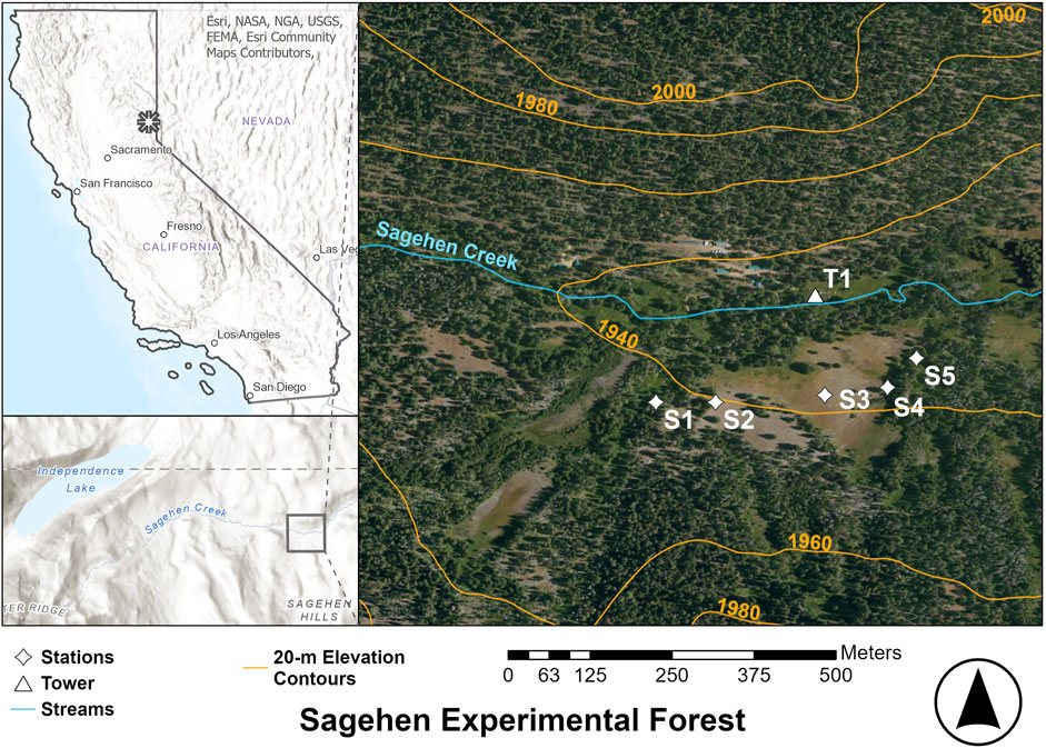
FIGURE 1. Sagehen Experimental Forest location in California (upper left), southeast of Independence Lake (lower left) with station locations near Sagehen Creek (right). Prevailing winds are WSW. (Figure author: Lauren Phillips).

A meadow located south of Sagehen Creek and the main building complex was chosen for the tower transect (Figure 1). The meadow covered approximately 3.2 ha with a 3° average slope. Line power was installed from an outbuilding through PVC conduit to each of five 6.1 m towers to power tower-mounted instrumentation. Towers were erected in locations representative of differing forest density along the WSW prevailing wind direction. The towers were fully installed by mid-January 2019. Station locations and elevations are shown in Figure 1 and enumerated in Table 1. Station 1 (S1) was located west of a meadow in dense trees 15–30 m tall; station 2 (S2) was at the upwind edge of the meadow, station S3 was in the center of the meadow, station 4 (S4) was at the downwind edge of the meadow and station 5 (S5) was in a canopy gap 15 m east of the meadow. S5 was positioned approximately 20 m north of the optimal position for flux footprint overlap with S4 to avoid an ephemeral swampy area, which may have otherwise biased resulting evaposublimation calculations. The topography along the transect sloped gently towards Sagehen Creek, approximately 100 m north of the transect.

TABLE 1

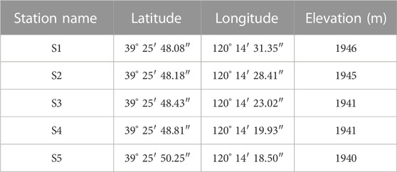
TABLE 1. Flux station locations.

2.2 Measurements

The five towers were equipped with different configurations of EC systems each year to characterize the variability of derived fluxes due to position with respect to the forest structure, wind direction and measurement height, given a limited set of instruments. Deployment configurations were optimized for measurements focused on horizontal variability across the tower transect during years 1 and 3, and vertical flux divergence at three stations during year 2. For brevity, winter seasons 2018–2019, 2019–2020 and 2020–2021 are hereafter referred to as Y1, Y2 and Y3. During Y1 and Y3, either a Campbell Scientific Irgason or EC150/CSAT3 pairing (generically referred to as “EC”) was mounted at a 6-m nominal height a.g.l. on each of the five towers. During Y2, an additional EC system was mounted at a 2.5-m height on towers S1, S2 and S3 with the trade-off that S4 and S5 were not equipped with flux instrumentation. ECs were mounted in the same orientation, perpendicular to the plumbline, such that systematic error due to orientation was not amplified (Frank et al., 2016). High-frequency data were collected at 20 Hz on CR3000 and CR6 data loggers (Campbell Scientific Inc., Logan, Utah) except for S4 and S5 on Y3, which were acquired at 10 Hz due to slower logger throughput (CR1000X, Campbell Scientific Inc., Logan, Utah) when collecting data at several timing intervals.

For all years and on all loggers, raw data were stored on flash media so that measurements could be quality assured before fluxes were computed. Omnidirectional sonic anemometers (81000VRE, RM Young) were mounted on a vertical boom at S1, S2 and S3 during Y2 and on all five towers for Y3 for improved resolution of the effect of canopy heating. Measurements from slow response instrumentation were collected at 20-s intervals and stored as 1-min averages. Slow response instruments included shielded thermohygrometers (Vaisala Model HMP-155) measuring air temperature and relative humidity, narrow field radiometers (Apogee SI-111) measuring snow and canopy emissivity with a 22° half angle field of view, snow depth sensors (SR-50A, Campbell Scientific Inc.), temperature probes (107, Campbell Scientific Inc.) to measure soil surface temperature, soil moisture and temperature probes (Decagon 5TM), LI-COR PAR pyranometers to measure downwelling insolation and 4-component radiation sensors (CNR4, Kipp & Zonen). Field cameras (Meidase SL122 Pro) were installed on each tower and equipped with 16 GB flash cards to document instrument and forest state at hourly intervals. A complete listing of instruments and locations is documented in field reports with the dataset in PDF format (see Data Availability Statement for dataset location). EC instruments were mounted on 1-inch (0.0254 m) diameter aluminum booms to minimize sway. Irgasons and EC150s were oriented perpendicular to the valley axis such that up-valley and down-valley wind directions were not obstructed by the mounting tower. Nominal positions of individual instruments for Y1 and Y2 are shown in Figure 2. The Y3 EC instrumentation is the same as Y1 but with the instrumented vertical boom shown for Y2 in Figure 2.

FIGURE 2

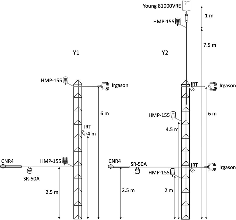
FIGURE 2. Diagrams of nominal instrument height a.g.l. on flux stations during Y1 and Y2. Instrument positions during Y3 are similar to Y2 but there was only one Irgason during Y3 and it was positioned at 6 m a.g.l.

Snow depth and snow water equivalent (SWE) transects were acquired with a depth probe and a Federal snow sampler (Osterhuber, 2014) during Y1 and Y2 at weekly to bi-weekly intervals in support of the NASA SnowEx campaign (e.g., Kim et al., 2017). SWE data collected at each station were interpolated in time and combined with snow depth measurements to derive SWE estimates at higher temporal resolution.

2.3 Methods

The spatial representativeness of fluxes derived from eddy-covariance methods relies on Taylor’s Hypothesis (TH) of frozen turbulence, which states that the total derivative equals zero (Stull, 1988):

$\frac{\mathit{d}\mathit{\xi }}{\mathit{d}\mathit{t}}=\frac{\mathit{\partial }\mathit{\xi }}{\mathit{\partial }\mathit{t}}+\mathbf{U}\frac{\mathit{\partial }\mathit{\xi }}{\mathit{\partial }\mathit{x}}+\mathbf{V}\frac{\mathit{\partial }\mathit{\xi }}{\mathit{\partial }\mathit{y}}+\mathbf{W}\frac{\mathit{\partial }\mathit{\xi }}{\mathit{\partial }\mathit{z}}=\mathbf{0},$

where $\xi$ is any scalar and mean wind components $\mathrm{U},$ $\mathrm{V}$ and $\mathrm{W}$ are oriented in the $x$, $y$ and $z$ directions, respectively. Typically, horizontal homogeneity of the landscape and turbulence stationarity are assumed such that horizontal derivatives of scalars are negligible and turbulence is evolving slower than a prescribed time averaging interval. When valid, TH provides a rationale to transpose a local time derivative measured on a tower to spatial derivatives representative of an area. A critical aspect of the notion of frozen turbulence is that the rate of change of turbulence is small relative to advection speed, so a given eddy does not significantly evolve in the time it takes for the eddy to propagate across a stationary sensor. Many studies have investigated the limits of TH and methods to quantify the range of valid length and time scales (e.g., Higgins et al., 2012; Higgins et al., 2013). For this investigation we use the turbulence intensity (TI) as a measure of TH conformity:

$\mathit{T}\mathit{I}=\frac{{\mathit{\sigma }}_{\mathit{M}}}{\mathit{M}},$

where $M$ signifies horizontal wind speed and ${\sigma }_M$ is the standard deviation of wind speed. A recommended range for discriminating the validity of Taylor’s hypothesis is TI < 0.5 (Willis and Deardorff, 1976). A flux measurement obtained with TI > 0.5 does not necessarily signify that calculated fluxes are invalid. Rather, TI gives a quantitative measure the degree to which turbulence is stationary and thus is a statistic related to the flux footprint.

Fundamentally, the eddy-covariance method captures vertical turbulent fluxes at the instrument location. An assumption that turbulence is sufficient to mix air parcels justifies a broader spatial representation of net vertical exchange of scalar quantities, such as moisture, or vector quantities, such as momentum. For EC deployments on tall towers, the ideal scenario is that turbulence is sufficient to mix the air (so the EC assumption is valid) but not so intense relative to wind speed that the TI test is exceeded. The EC method uses high-frequency measurements to quantify vertical exchange over a prescribed averaging interval. Temporal perturbations in temperature ($T^{\prime }$) and vertical wind speed ($w^{\prime }$) contained in eddies are therefore responsible for the kinematic vertical sensible heat flux, determined as (Stull, 1988):

$\mathit{K}\mathit{S}\mathit{H}=\overline{{\mathit{w}}^{\prime }{\mathit{T}}^{\prime }},$

where the overbar signifies a time average. The specific heat of air and air density are then used to convert kinematic units to flux units in $W{m}^2$. Likewise, the kinematic vertical moisture flux is computed as:

$\mathit{K}\mathit{L}\mathit{E}=\overline{{\mathit{w}}^{\prime }{\mathit{q}}^{\prime }},$

where ($q^{\prime }$) are moisture perturbations relative to the time average and air density and the latent heat vaporization of water are used to convert kinematic units to $W{m}^2$. Many corrections may be applied to kinematic fluxes depending on the environmental conditions and deployment considerations. The gamut of possible corrections is beyond the scope of this paper and is documented in other sources (e.g., Massman and Lee, 2002). Specific corrections applied to data acquired in this experiment are documented in Section 2.4.

Typically, EC equipment is deployed high above the forest canopy with the goal of integrating heterogenous sources within the tower footprint to obtain fluxes representative of a large area. However, our approach was to deploy multiple EC stations at a lower height with small, proximal footprints so that we could disaggregate near-field flux sources. That is, when flux footprints are oriented streamwise, a change in flux relative to an upwind station can be attributed to a local source. For this experiment, EC systems were mounted high enough to avoid snowfall inundation or anomalous flux results due to proximity of the snow surface (e.g., by pressure fluctuations). An additional concern for this gently sloping valley site was freezing fog, which was not uncommon in winter, and would deposit on the open path gas sensor, obstructing measurements. Higher positions on the tower corresponded to stronger winds, which help mitigate deposition on the instruments while increasing tower footprint size relative to a lower instrument height. The compromise height of 6 m a.g.l. positioned the EC system roughly 4 m above the historical average maximum snow depth. Heaters on the EC systems were not used because the power demand exceeded the amperage supply. Not heating the infrared sensor resulted in longer data outages while avoiding potential fictitious fluxes caused by the heating element. Relatively low height and positioning the EC systems below canopy top constrains the fetch relevant for surface flux determinations. While a small fetch is typically unadvised because it means the flux calculations apply to a small area, this consideration was applied in this experiment to discriminate the influence of near-field forest canopy structure on calculated fluxes. Footprint estimates for each station are provided as Supplementary Materials.

We employed a boosted regression tree (BRT) algorithm (Matlab model LSBoost, R2022a) to quantify environmental parameters that are most predictive of evaposublimation. Unlike multilinear regression analysis, a BRT accommodates observed non-linear contributions to fluxes, some of which are discussed in Section 3.1. Comparable measurements at each station were taken at the same height a.g.l. although there is some potential for bias in BRT analyses due to differences in snow depth. Predictive parameters included daily averaged quantities for downwelling shortwave radiation, 6-m air temperature, 6-m relative humidity, 6-m wind speed, and snow skin temperature. We selected these variables based on their effects on snowpack ablation, data quality, and data availability across stations and study years. Output parameters of daily-averaged SH and LE (sensible and latent heat fluxes in W m², respectively) were compared independently at each station. Even with a large data set, daily sums of 10-min averaged flux data from three winters that were used for the BRT analysis represent a relatively low volume of data to build a BRT, so the model was trained with 90% of the data and the remaining 10% were used to compare predictions with measurements. The BRT was run over the time span that snow was on the ground as identified by snow depth measurements.

2.4 Data processing

Raw data were filtered as the initial step of a multistep data processing pipeline. Data values that exceeded a predefined plausibility range were marked as invalid. Data were checked for time continuity and gap-filled with NaN values to form continuous, time-consistent records. Flux data were processed with a batch script that invoked the EddyPro v7.0.7 software package (LI-COR Inc., Lincoln, Nebraska) independently for each week such that the height of the EC system above the surface could be initialized from snow depth measurements. Diagnostic flags reported by Irgasons and RM Young sonics were exercised in EddyPro with a requirement that no more than 10% of the data records were either missing or out-of-range for each time average. An independent signal strength cutoff was implemented for each Irgason due to differences in raw signal strength of each gas analyzer. EddyPro was configured to produce both 10-min and 30-min averaged quantities such as sensible heat flux (SH), latent heat flux (LE), flux footprint size, and spectral statistics. A short averaging interval was chosen to minimize contamination by larger scale processes (Mahrt and Vickers, 2006; Oldroyd et al., 2016).

Snow depth measurements for Y1 were gap-filled from initial snowfall up to January 12 by interpolation with snow depth measurements at the Independence Creek SNOTEL site (elevation: 2128 m, distance: 7.5 km). The Independence Creek SNOTEL site had a very similar snowpack evolution pattern to station S3 in Y1. Maximum downwelling solar insolation measured by PAR sensors for Y1 were normalized to the CNR4 sensor at S3 on cloud-free days (January 24, 25, 27; February 22; March 15, 16, 18, 31; April 18, 22, 25, 27, 28; May 4) to minimize the impact of systematic error in PAR sensor data.

3 Results

3.1 Climatology

We first present onsite climatological data for Y1-Y3 to contextualize sensible and latent heat flux results presented in Section 3.2.

3.1.1 Snow depth

Snow depth timeseries at the five instrumented towers for the three winter seasons display year-over-year commonalities as well as significant differences (Figure 3). Frequent storm cycles with multiple rain-on-snow events during Y1 contrasted with fewer, large magnitude storms during Y2 and Y3. For all three winter seasons, snow depth at densely forested S1 was lower than the other four stations as was the snowpack ablation rate during spring. Snow density at S1 (not shown) was greatest for all years due to canopy unloading (Hedstrom and Pomeroy, 1998) and snowmelt drip from surrounding trees that refroze in the snowpack. For Y1, the snowpack was sufficiently deep and ablation rate was sufficiently low in the shade of dense trees that snow persisted longest at S1 and melted out earliest at S3. Isolated snow patches persisted in shaded areas between stations even longer than at S1 during Y1. For the lower snowfall year, Y2, a late, high accumulation storm event had a similar effect as high accumulation year Y1 with snow persisting longest at S1. In Y3, snow disappearance date was similar at S1 and S3. Fewer storms with longer periods of fair weather yielded greater potential for melt and evaposublimation during Y2 and Y3. These results suggests that, at this upper montane elevation, cumulative evaposublimation and snowpack disappearance date for open vs. dense canopy depends, in part, on year-to-year differences in total accumulation timing and amount. This result refines those of Roth and Nolin (2017), which did not qualify the result that differences in snowpack melt-out date for open vs. canopy-covered areas also depends on accumulation timing and amount. Increasing insolation with increasing zenith angle caused ablation curves for all sites to converge except for the densely forested station, S1.

FIGURE 3

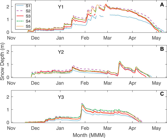
FIGURE 3. Snow depth measurements for each winter season at all five stations. Early season snow depth until 12 Jan 2019, for Y1 was interpolated from a nearby SNOTEL site (Independence Creek, Site 540, elevation: 1961 m).

3.1.2 Winds

The wind rose in Figure 4A is based on 1-min averaged winds at 6-m height for the open site (S3) during Y1 and shows a WSW prevailing wind direction, consistent with the along-valley wind direction observed at T1 the previous year that informed the experiment design. Wind direction for Y2 and Y3 was similar to that in Y1 at all towers (not shown) with subtle differences between stations due to canopy deflection and nocturnal drainage flow direction. The standard deviation of wind direction has been shown to be important for turbulent exchange at low wind speed (Mahrt et al., 2013; Freundorfer et al., 2019). However, high wind direction variability at low wind speed coincided with smaller LE fluxes (e.g., during nocturnal submesoscale events) compared to daytime values so the focus of this analysis is on daytime flux processes. As expected, wind speed was greatest at stations most exposed to the prevailing wind (e.g., S3) and lowest at the station in dense trees (S1) (Figure 4B). Bole space (the space between the snow surface and bottom of the canopy) was negligible for the trees at the experiment site so near-surface winds at S1 were weaker than mid-canopy level at all sites (not shown). For all sites, the composited wind speed was greater during the daytime than nighttime as shown in Figure 4B due to insolation driven spin-up. With low wind speed and shallow slope, air convergence due to local terrain slope is deemed minimal at this site. Wind speeds in this forested valley site were significantly lower than those at ridge-level so the corresponding evaposublimation rate was likely reduced relative to more exposed locations.

FIGURE 4

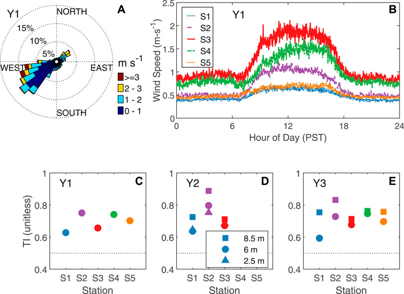
FIGURE 4. Y1 windrose for station S3 is shown in panel (A). Y1 composite of 1-min averaged wind speed at 6 m nominal height a.g.l. at each station in panel (B). In lower panel, average turbulence intensity (TI) for each station and each year.

Seasonal mean TI was computed from 1-min averaged wind speed at each sonic anemometer for each year of this investigation and plotted in Figures 4C–E. The lowest TI was found at S1, where the canopy was dense enough that turbulence strength had dissipated before the air stream reached the sensor giving a relatively small numerator in the TI calculation, even with low windspeed. TI was greater at all stations at higher positions a.g.l. (but still below canopy top) indicating that turbulence was increasing with height and consistent with shear generated turbulence at the top of the canopy. Lower TI at lower height does not indicate a larger flux footprint. Rather, it indicates that a larger fraction of flux is caused by an eddy size distribution that is shifted towards smaller eddies. For all stations, TI was above the 0.5 cutoff suggested by Willis and Deardorff (1976), challenging the frozen turbulence assumption of TH. Large TI does not invalidate fluxes calculated by eddy covariance but rather limits the length scale over which the flux determinations apply. The assumption that daytime turbulence is sufficient to measure fluxes by EC methods remains valid, therefore, we conservatively constrain the flux footprint to an area smaller than the distance between towers (Baldocchi, 1997; Schmid, 2002).

3.1.3 Solar insolation

Downwelling solar radiation at each station, shown in Figure 5A for clear-sky days February 22 and April 28 during Y1, exhibited the effect of canopy cover fraction. Similar to wind speed, solar insolation was largest at S3, smallest at S1, with the remaining stations having intermediate values that depended on southerly forest structure. As the solar zenith angle increased after the winter solstice, solar insolation correspondingly increased in importance as a driver of evaposublimation. As shown in Fig 5b, S1 had the smallest absolute change in solar insolation with seasonal progression because the canopy was sufficiently dense to nearly continuously shade that site even at higher zenith angles. The canopy gap at site S5 was large enough that solar insolation significantly increased as zenith angle decreased so it experienced the largest seasonal change in downwelling radiation. Solar insolation at S3 was greatest throughout the entire winter season. S2 was located on the western edge of the meadow and experienced greater solar insolation midwinter than S4, which was located on the eastern edge of the meadow. As the solar zenith angle increased in spring, the magnitudes of solar insulation as S2 and S4 reversed due to relatively more shading at S2 later in the day. This result highlights how minor differences in canopy structure and large differences over small distances consequentially impact surface energy balance. The variability of solar insolation between stations suggest that we have captured a broad cross-section of solar insolation conditions across the forests of the Sierra Nevada Mountains.

FIGURE 5

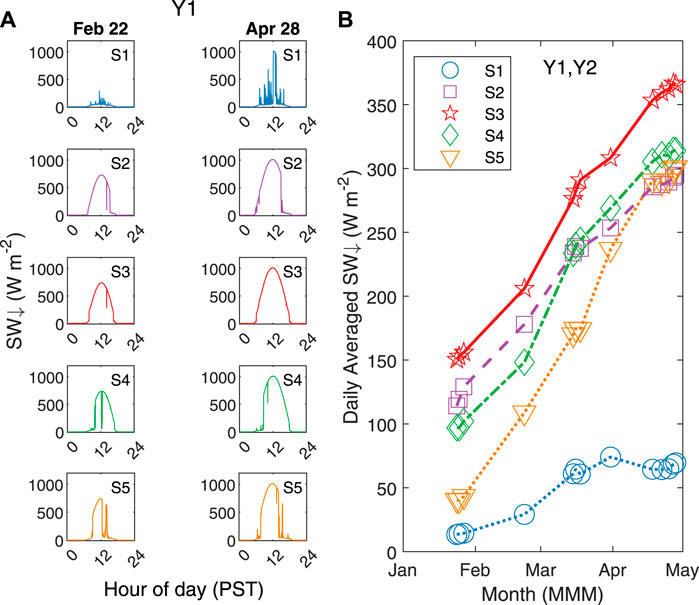
FIGURE 5. Shading strongly influenced insolation at each station. In panel (A), 1-min averaged downwelling broadband radiation measured at each station on clear-sky days 22 Feb 2019 (column 1) and 28 April 2019 (column 2). Daily averaged downwelling solar radiation during representative clear-sky days at each station on Y1 and Y2 [panel (B)].

3.1.4 Canopy heating

During Y2, five Apogee SI-111 IRTs (infrared temperature sensors) were deployed at stations S1, S2 and S3. At stations S1 and S2, one IRT was oriented towards the snow and a second IRT was oriented towards the canopy. At S3, a single IRT was oriented towards the snow surface. Field cameras pointed at the canopy were used to verify the presence/absence of snow in the canopy. In Figure 6, 4-day composites of skin temperature of the canopy and snow surface are compared for stations S1, S2, and S3 during time periods when snow was present in the canopy (panel A) and a different 4-day time period when the canopy was snow-free (panel B). Solar insolation heated the canopy to temperatures ∼ 5 °C (at S2) and ∼10 °C (at S1) during the snow-free period relative to the time when snow resided in the canopy. Canopy heating at S2 was smaller relative to S1 because greater air flow (wind speed) more efficiently ventilated the canopy. Using the Stefan–Boltzmann law, a 5 °C increase in emission temperature above freezing corresponds to a 24 W m^-2 radiant flux increase (at S2) and likewise, a 10 °C increase in emission temperature above freezing corresponds to a 49 W m^-2 radiant flux increase (at S1). Both of these radiant flux increases are significant relative to SH and LE flux magnitudes and contribute to snow ablation at the tree scale. A canopy warmed by solar insolation also warmed the air around it by conduction and convection, thereby increasing evaposublimation rates. Similar to Storck et al. (2002), canopy-intercepted snow at this lower elevation melts and sloughs, so it is exposed to ventilation for a shorter period of time relative to higher elevation subalpine regions (e.g., Montesi et al., 2004; Molotch et al., 2007), thereby decreasing the fraction of snow sublimated from canopy. The impact of competing processes of higher evaposublimation rate and lower exposure time for this montane forest site as compared to an alpine environment was not addressed by this experiment and merits further investigation. We attribute the 0.5°C emission temperature of the snow at S1 to forest litter from nearby trees accumulating on the snow surface, which lowers the albedo, increases net shortwave radiation, and warms the snowpack.

FIGURE 6

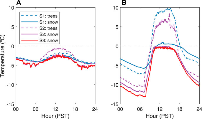
FIGURE 6. Composited IR emission temperature of targets when trees are snow covered [panel (A)] and snow-free [panel (B)].

3.1.5 Soil moisture

Rain-on-snow (ROS) events are an increasingly common feature of atmospheric rivers (Zhu and Newell, 1994) for the maritime snowpack in the upper montane region of the Sierra Nevada Mountains but uncommon for continental and alpine snowpacks. These events have consequential near-term effects for SWE, runoff, and snowpack stability as well as longer-term effects on snowpack longevity and vadose zone recharge (Kirchner et al., 2020). Figure 7 compares the effect of hydrologically significant ROS events on subnivean soil moisture for high snow Y1 (panel A) with low snow Y2 (panel B) at site S2. For the purposes of this study, we define hydrologically significant ROS events as storms with air temperature above 0 °C and with a stream gage response in Sagehen Creek of at least 0.5 orders of magnitude above the baseflow flux (see analysis in Supplementary Materials). Frequent warm storm cycles during Y1 produced multiple ROS events. The resulting pressure head at the base of the snowpack was sufficient to overcome adhesive soil properties so water percolated through the soil resulting in “breakthough” curves. These breakthrough curves indicate active snowpack drainage, compared with the infrequent storm cycle during Y2 for which breakthrough curves are less evident. Sites S1, S3, S4, and S5 also had breakthrough curves at 16 cm depth but tended to saturate at the 66 cm depth (not shown) as the Y1 winter season progressed. During Y2 and Y3, the soil did not saturate at 66 cm depth at any time at stations S2, S4 and S5. These data, combined with hydrographs from a gage on Sagehen Creek (shown in Supplement) indicate both increased percolation and SWE loss by ROS events. ROS events transfer water formerly contained in the snowpack to the atmosphere by latent heat flux (Marks et al., 1998) and to the soil by percolation and snowmelt. The corresponding loss of SWE reduced a near-term source for evaposublimation while soil hydration increased a source of evaposublimation after the snowpack had dissipated with poorly understood consequences for the hydrologic cycle. In contrast with a maritime snowpack, continental snowpacks rarely experience ROS events thus limiting midwinter vadose zone recharge potential.

FIGURE 7

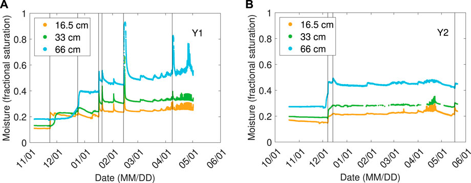
FIGURE 7. Normalized soil moisture at 16.5 cm, 33 cm and 66 cm depths at station S2 for Y1 [panel (A)] and Y2 [panel (B)]. Soil moisture increased during atmospheric river events and with depth due to close proximity to the water table. ROS events are indicated by vertical lines.

3.2 Sensible and latent heat fluxes

The climate data analysis for the maritime, montane site in the present study yields consequential process differences compared with higher elevation subalpine and alpine sites (e.g., Marks and Dozier, 1992; Musselman et al., 2008; Mott et al., 2011). Our results suggest that conclusions pertaining to the relative importance of factors that drive fluxes at alpine and subalpine sites may not directly extend to maritime, montane sites. The remainder of the results section is dedicated to evaposublimation calculations as they pertain to upscaling local fluxes to a larger domain.

3.2.1 Energy balance

Energy balance (EB) closure refers to a balance between net radiative inputs (such as shortwave and longwave radiation) and ground heat flux relative to fluxes of heat and moisture. Horizontal homogeneity, which is lacking for this experiment site, is an implicit assumption when considering a 1-D model of energy balance. Typically, the sum of vertical fluxes is less than net radiative inputs so the question arises: what happens to the unaccounted for radiative energy? Energy balance closure is rarely achieved even for idealized experimental designs (Foken and Oncley, 1995) and it is not observed in this experiment. We examine a 7-day period (26 March 2021 through 1 April 2021) of nearly identical diurnal conditions to gather sufficient statistics to examine the nature of the lack of EB closure. The snowpack was rapidly ablating during this time period.

Radiative inputs measured by a 4-component radiometer and averaged to 30-min averages are shown in Figure 8A for station S1, located in dense trees. For comparison, identical measurements from another 4-component radiometer at station S3 are shown in Figure 8B. The shape and amplitude of the SW $\downarrow$ component in Figure 8B indicates clear-sky conditions with the jagged shape of the SW $\downarrow$ component at S1 in Figure 8A indicating intermittent canopy shading. Low SW $\uparrow$ measurements at S1 due to shaded snow having pine needles and other canopy debris contrasts with much higher SW $\uparrow$ values in a snow-covered open area. Diurnal variations are evident for both LW $\downarrow$ and LW $\uparrow$ components in both the open and forested site. At S3, LW $\uparrow$ was larger than LW $\downarrow$ due to the snowpack that was relatively warmer than the integrated radiance of the atmosphere. At S1, LW $\uparrow$ and LW $\downarrow$ are similar because the snowpack radiant temperature is similar to the lower canopy radiant temperature.

FIGURE 8

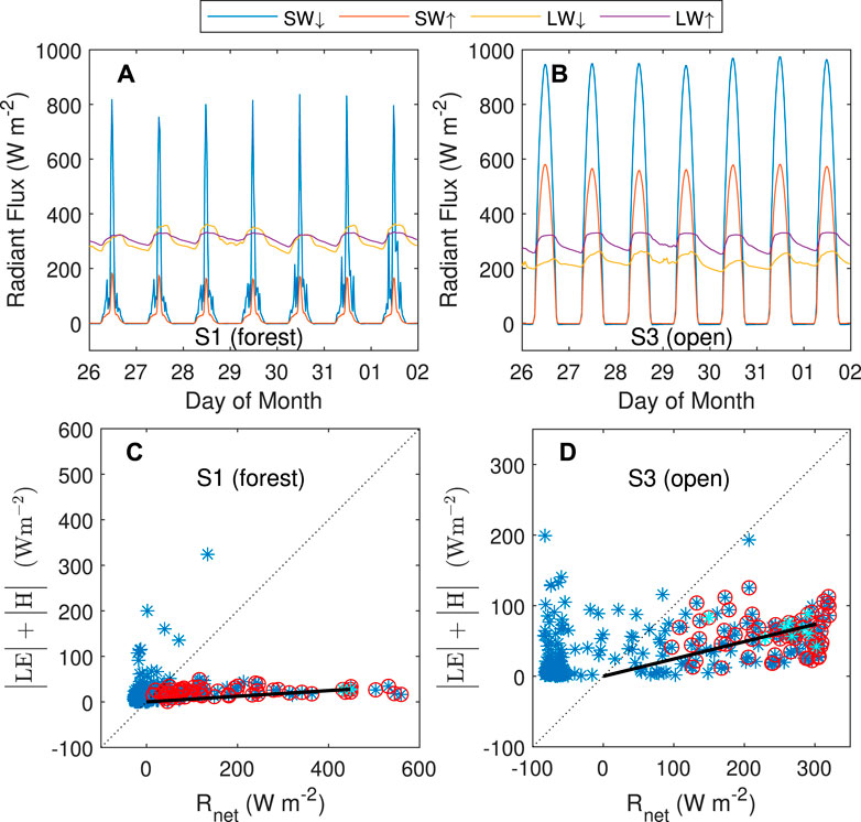
FIGURE 8. Radiative flux components (top row) for the forested site, S1 (left column), and the open meadow site, S3 (right column) during a series of clear-sky days. Correlation plots showing the sum of turbulent sensible and latent heat flux magnitudes against net radiative fluxes (bottom row).

The degree of imbalance between net radiation and sensible and latent heat fluxes at S1 and S3 is expressed in Figures 8C,D, respectively, as the difference between measurements and the 1:1 dotted line. In both figures, 30-min averages are indicated by a blue asterisk. Measurements acquired during the convective part of the day (11AM to 4PM, PST) are circled in red. Measurements corresponding to average wind speeds exceeding 3 m s^-1 are cyan colored. The 3 m s^-1 threshold was arbitrarily chosen to denote windy periods for which there is an expectation that winds will more efficiently mix the roughness sublayer, improving the basis for EC measurements. For both sites, the sum of latent and sensible heat fluxes is less than net radiation during the day. The assumption of 1-D EB closure is better at station S3 than S1, although neither station approaches the 1:1 line. Lack of EB closure is due to several unaccounted processes including: phase change from ice to liquid (meltwater runoff), local exchange processes across horizontal gradients (Morrison et al., 2021), horizontal variability in local storage (Higgins et al., 2012) and exchange processes at larger scales (Foken, 2008). Increased daytime winds persist beyond the timeframe of positive net radiation and contribute to the non-convective time period to the left of the 1:1 dotted line for which environmental fluxes exceed net radiation. Lacking a full accounting of energy transfers, it is not clear the degree to which 30-min averaged EC fluxes do not fully capture the magnitude of sensible and latent heat processes. What is evident, is that fluxes inferred from net radiation would overvalue flux magnitudes unless other measures of energy balance, which are poorly bounded, are obtained. Figures 8C,D additionally indicate that daily-averages will improve EB convergence relative to 30-min averages.

3.2.2 Interannual SH and LE variability

Cumulative, daily-averaged sensible and latent heat fluxes for each station and each year are presented in Figure 9 with the convention of positive values representing a flux into the atmosphere. The lefthand column of Figure 9 shows cumulative sensible heat flux values for Y1, Y2, and Y3 and the righthand column shows cumulative latent heat flux values for each year. These data are quality-controlled but not gapfilled, which produces data gaps and the staggered appearance of the line plots. These non-gap-filled data were used to develop environmental response functions (ERFs), so the resultant ERFs do not rely on interpolated data. Comparing matching days for which we have data, the evaposublimation rates were greater during Y2 and Y3 relative to Y1, suggesting that infrequent storm cycles accompanying low precipitation years lead to greater evaposublimation totals and a greater fraction of SWE loss. This effect exacerbates low water storage in drought years.

FIGURE 9

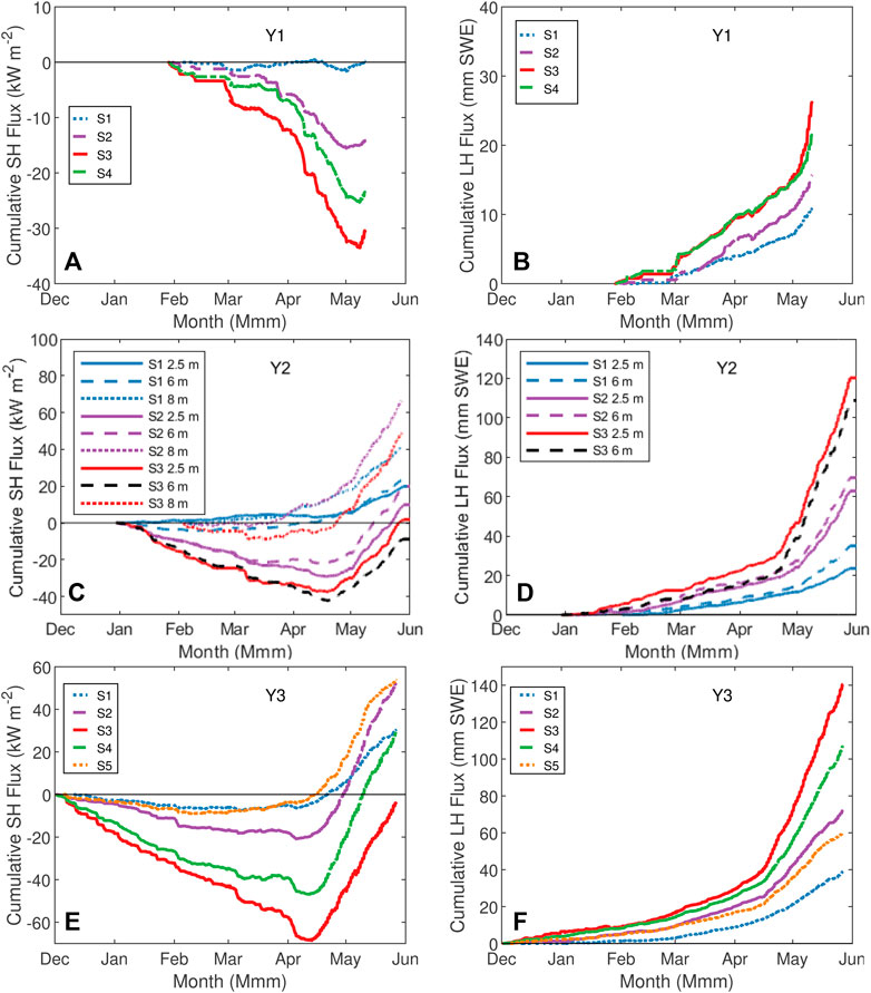
FIGURE 9. Cumulative daily-averaged sensible and latent heat fluxes for Y1, Y2 and Y3. Poor quality fluxes were removed from these analyses resulting in a jagged appearance in the line plots.

For each of the 3 years of the study, near-surface sensible and latent heat fluxes were largest at S3 (in the middle of the meadow). We attribute larger latent heat flux at S4 than S2 to stronger prevailing winds and enhanced turbulence downwind of meadow relative to upwind (Figure 4B). The difference in measured latent heat fluxes between S4 and S2 increased late in Spring as insolation at S4 surpassed insolation at S2 (Figure 5B) causing increased turbulent exchange.

Station S1 (in dense trees) recorded the smallest near-surface flux magnitudes, however, fluxes increased with height as shown in the Y2 plots (Figure 9, panels C, D). Increasing flux with height in the canopy is consistent with others’ results (e.g., Gao, 1995; Foken, 2017) as increased ventilation and increased solar insolation align. Evaposublimation at S1 is presumed to be highest in the canopy crown where both wind and solar insolation are maximized but only when snow or water were in the canopy. Immediate post-storm evaposublimation estimates from the canopy before snowmelt were not well-captured in this experiment because of inundation of the open path sensors. Sensible heat fluxes at S3 are essentially the same when measured at 2.5-m and 6-m heights (Figure 9C) while the snowpack is contiguous but sensible heat fluxes are weaker when measured at 8 m. This observation does not exhibit a constant-flux surface layer that is more typical of idealized sites. Rather, the constant fluxes at the lower levels are influenced by an elevated temperature inversion that is caused by canopy heating extending into the meadow. Unlike measurements at sites influenced by the forest canopy, latent heat flux at station S3 is consistently larger at 2.5-m height than at 6-m height.

The shapes of cumulative flux curves in Figure 9 are similar year-to-year. The sensible heat flux curves show quasi-linearly decreasing values until snowmelt (see Figure 3), at which time the slopes abruptly changed signs as the soil surface warmed and reversed the near-surface temperature gradient. The latent heat flux curves have modestly increasing slopes until snowmelt, at which time slope increases to a steep, linear trend. We will utilize similarity of these curves when developing ERFs in the Discussion section.

3.2.3 Boosted regression tree analysis

Results of a BRT analysis are shown in Figure 10. As one might expect, the cumulative predictor was generally greatest in the open (S3) and lowest in the trees (S1, S5), although evaposublimation predictability at station S3 was less than S2 or S4 during Y1. This result underscores the difficulty of inferring fluxes at subcanopy stations from other measurements. Previous experiments in subalpine and alpine environments have shown that solar insolation and wind speed, respectively, are the most important parameters for producing evaposublimation. Ranking the magnitude of the predictive parameters in Figure 10 yields the result that SW $\downarrow$ >6-m wind speed > 6-m relative humidity > surface emission temperature >6-m air temperature. These results do not dispute previous findings but do qualify and add nuance to previous results.

FIGURE 10

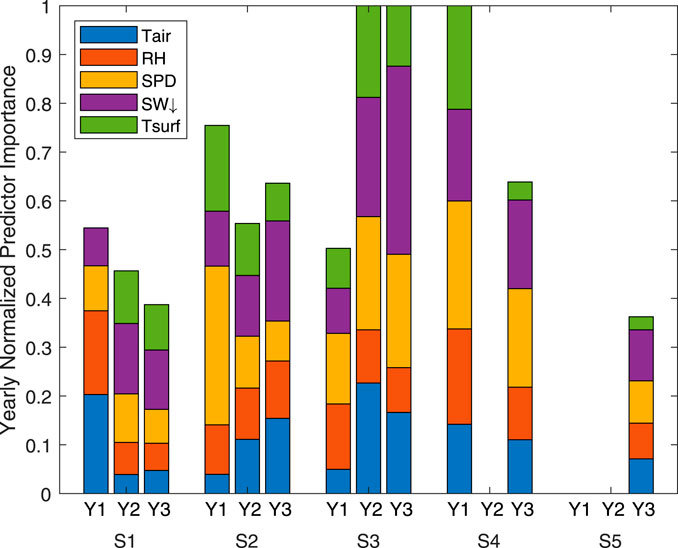
FIGURE 10. Relative value of predictors for latent heat flux at each flux station for each winter season. Predictors include 6-m air temperature (Tair), 6-m relative humidity (RH), 6-m wind speed (SPD), downwelling shortwave radiation (SW) and surface IR emission temperature (Tsurf). The predictors are seasonally normalized by the best fit yielding a maximum value of 1.

The predictive strength of the BRT parameters varied depending on wintertime storm frequency. For example, relative humidity and air temperature gained relevance compared to the other parameters during the more overcast winter, Y1. Solar insolation was less predictive of evaposublimation during Y1 than was wind speed. This result is likely because evaposublimation may be high with clear skies but also potentially high during overcast periods accompanying warm air temperatures and high wind speeds, which were more common during Y1. During low precipitation years, solar insolation at forested stations S1 and S5 was more predictive of evaposublimation than air temperature. Conversely, air temperature was the most predictive parameter at station S1 during high precipitation year Y1. Comparing stations S2 and S4 on either side of the meadow, SW $\downarrow$ was more predictive at S2 and wind speed was more predictive at the windier and more shaded S4 during low precipitation years. During Y1, wind speed was the most predictive parameter at both stations.

Canopy skin temperature was the least valuable predictor of subcanopy evaposublimation for stations not in proximity to the canopy and therefore was not included in the BRT. Based on results in Sections 3.1.3 through 3.1.5, we assess that skin temperature of the canopy is very important when the canopy warms after a snowfall, producing high evaposublimation rates. However, unlike continental forests, the time period over which canopy-intercepted snow experiences high evaposublimation rates is limited because much of the canopy-intercepted snow partially melts and sloughs to the surface.

We note that BRT technique has been previously employed for gap-filling flux calculations for a larger data set (e.g., Shang et al., 2020) and spatially distributed SWE estimates (Molotch et al., 2005). However, the emphasis of this paper is to improve the spatial resolution of evaposublimation estimates, so we instead utilized quality-controlled flux determinations to examine variability in the predictive strength of common field-based and model simulated parameters.

4 Discussion

The similarity in form of SH and LE curves in Figure 9 suggest that similar evaposublimation processes occur at each station but at different rates that depend on forest structure. We therefore explore developing an environmental response function (ERF) that can be used to downscale model simulated evaposublimation rate to sub-stand scale. The goal is to distinguish subcanopy evaposublimation from model-derived and remotely-sensed sources to have a product that can be used to gauge the evolution of subcanopy aridity. That is, models can use MOST to produce fluxes over open areas and then use an ERF to estimate subcanopy fluxes where MOST assumptions are routinely violated. Daily-averaged and quality controlled latent heat fluxes calculated at each station were used to produce the ERF. The ERF diagnoses the fraction of subcanopy evaposublimation relative to an open area for a location with a given canopy density. That is,

$\mathit{f}\left({\mathit{c}}_{\mathit{f}},\mathit{R}\downarrow ,\overline{\mathit{M}},\mathit{D}\mathit{I}\mathit{R},\mathit{T}\mathit{I},\mathit{T},\mathit{e},\dots \right)={\mathit{L}\mathit{E}}_{\mathit{s}\mathit{u}\mathit{b}\mathit{c}\mathit{a}\mathit{n}\mathit{o}\mathit{p}\mathit{y}}/{\mathit{L}\mathit{E}}_{\mathit{o}\mathit{p}\mathit{e}\mathit{n}}$

Where $\mathit{f}$ is a fraction that is a function of canopy density (${\mathit{c}}_{\mathit{f}}$), downwelling shortwave radiation ($\mathit{R}\downarrow$), wind speed ($\overline{\mathit{M}}$), wind direction ($\mathit{D}\mathit{I}\mathit{R}$), turbulence intensity, air temperature, vapor pressure and other state variables. ${\mathit{L}\mathit{E}}_{\mathit{s}\mathit{u}\mathit{b}\mathit{c}\mathit{a}\mathit{n}\mathit{o}\mathit{p}\mathit{y}}$ is the daily averaged latent heat flux in the subcanopy and ${\mathit{L}\mathit{E}}_{\mathit{o}\mathit{p}\mathit{e}\mathit{n}}$ is the daily averaged latent heat flux at a nearby open area, station S3 in this case. Accounting for canopy fraction, an ERF was determined empirically with a function fit to data shown in Figure 9. There is not a defined mapping between canopy fraction at the 30-m scale and experiment sites that have a canopy fraction at higher resolution. To address this scale mismatch, we estimate the canopy fraction as $\left(1-SVF\right)$, where $SVF$ is the sky view factor at each site. The sky-view factor is estimated as the average sky-view factor in each of eight compass directions separated by 45° taken at a standing height of 1.5 m.

To estimate $\mathit{f},$ we bin-averaged daily latent heat flux data in Figure 9 and plotted the results as a function of the latent heat flux measured at S3 in Figure 11A. S3 data plotted against itself (red line) serve as a reference for comparison with other stations. As shown in Figure 9, S1 had the lowest LE values relative to S3 followed by S2 and S4. Stations S2 and S4 had similar sky view fractions but S4 had generally larger LE fluxes. Insolation and turbulence intensity are similar (Figure 5B, and Figures 4C, E) but wind speed at the downwind site (S4) is significantly greater than at S2 (Figure 4B). We attribute the larger LE fluxes at S4 as mostly due to wind speed, which, because of canopy topology, is a function of wind direction.

FIGURE 11

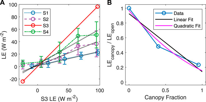
FIGURE 11. Bin-averaged latent heat fluxes at each station as a function of latent heat fluxes at S3 using Y1 and Y3 data sets [panel (A)]. Black dotted lines signify linear fits. The slope of the line from panel (A) is plotted as a function of canopy fraction in panel (B). The linear fit is y=0.79x + 0.93 and the quadratic fit is y=0.35*(x-1.66)².

In Figure 11A, deposition occurs when the latent heat flux is negative. We note that when deposition occurs, site S3 is not predictive for LE fluxes at the other stations (the slope of the line is flat). Canopy decoupling is common in stable conditions, so this result makes sense (Thomas et al., 2013). Therefore, the remainder of the analysis is focused on positive values of LE fluxes. The dotted black lines in Figure 11A show linear curve fits for each station, ignoring negative bin-averaged data. The respective slopes of these lines are plotted against canopy fraction in Figure 11B. In Figure 11B, the slopes for stations S2 and S4 are averaged because we lack model-simulated wind direction data with sufficient resolution to apply an ERF across a landscape. The analysis could therefore be improved with high-resolution wind direction information, either modeled or measured. The quadratic fit in Figure 11B is superior to the linear fit. This result is expected because of the non-linear influence of solar insolation and wind speed near the forest edge. Now that we have a relationship that diagnoses the fraction of subcanopy evaposublimation to evaposublimation in open areas as a function of canopy fraction, we can apply this ERF to a larger forested area in the region.

Specifically, the ERF process is to:

1) Downscale the ERA5-Land latent heat flux product to the 30-m resolution of the NLCD 2016 USFS Tree Canopy Cover product.

2) Normalize the tree canopy cover product to values between 0 and 1 and invert so that 1 corresponds to open areas and 0 corresponds to pixels with the highest possible canopy cover density.

3) Multiply the downscaled ERA5-Land product from step 1) by the normalized tree canopy cover product in step 2)

4) Use LE flux measurements to produce best-fit curves that diagnose the fraction of subcanopy LE flux relative to a station in the open. The quadratic fit in Figure 11B was used in this study.

5) Use the best fit curve from step 4) and the original ERA5-Land latent heat flux product to calibrate the high-resolution product from step 4).

The final product from step 5) is a 30-m resolution map of daily subcanopy latent heat flux estimates.

A sample ERA-Land daily-averaged latent heat product over the Central Sierra Nevada for 1 April 2020, is contoured in the background of Figure 12 in a rectilinear mapping projection. The daily average LE flux was calculated by summing 24 hourly products and performing time unit conversions. For the Central Sierra region, the original ERA-Land latent heat product has a grid size of 25.6 km latitude and 19.8 km–20.7 km longitude (using an arc length measurement). The NLCD 2016 USFS Tree Canopy Cover product for the same region is overlain in Figure 12 in its native rectilinear mapping projection. After applying the ERF process, the downscaled evaposublimation rates from step 5) are mapped in Figure 13. This product represents surface evaposublimation from open and canopy-covered areas. Evaposublimation from large open areas such as Lake Tahoe (lower right area in Figure 13) is no better (or worse) than interpolating the ERA-Land product and suggests an alternate function pertinent for non-forested areas. A comparison of Figures 12, 13 shows the potential for estimating flux heterogeneity by applying an informed combination of field-based data, model simulations, and remotely sensed products.

FIGURE 12

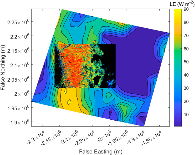
FIGURE 12. ERA5-Land latent heat product for 1 April 2020 with inset containing the NLCD Tree Canopy Cover product for a region spanning the Central Sierra Nevada. The outline of Lake Tahoe is evident in the lower right corner of the canopy cover product. Black color represents no canopy cover and red colors represent high canopy density.

FIGURE 13

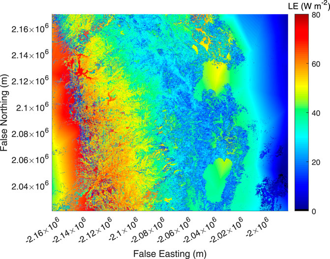
FIGURE 13. 1 April 2020 subcanopy LE flux determined by merging ERA5-Land product with the canopy cover data set and applying an ERF to calibrate the result. The final map has 30-m resolution.

5 Conclusion

A field-based experiment was performed over three consecutive winter seasons to improve understanding of subcanopy evaposublimation of a montane, maritime environment. A novel experiment design enabled discriminating near-field evaposublimation sources across a broad range of canopy densities. The intensity of processes that generate evaposublimation in this montane environment contrasts with subalpine and alpine regions. Similar to a subalpine environment, canopy-intercepted snow experienced high sublimation rates. However, unlike its subalpine counterpart, canopy exposure time was constrained when post-storm solar insolation and warm temperatures produced throughfall, melt and refreeze. Frequent atmospheric rivers during the high accumulation year partially ablated the snowpack, transferring water from the snowpack to the vadose zone. This process occurred rarely in low accumulation years in this study and has implications for late season subcanopy aridity. In the high accumulation year (Y1), the snow melt-out date in the dense forest occurred later than in the open area as shading from solar insolation later in the season became more significant relative to other ablation processes.

Low frequency meteorological measurements were used with 10-min flux averages to construct regression trees that diagnosed daily-averaged sensible and latent heat flux for each station. This methodology of combining data products to diagnose spatio-temporal distributions of sensible and latent heat fluxes accommodates non-linearities in processes that ablate snow in forested regions. Comparing regression tree results between three winter seasons enabled a nuanced assessment of subcanopy flux processes. Similar to results for subalpine and alpine environments, solar insolation and wind speed were found to be dominant factors for evaposublimation. However, during the high accumulation year, wind was a stronger predictor for evaposublimation than solar insulation at the montane site. During the low accumulation years, the snow skin temperature was more predictive of evaposublimation than air temperature under a dense forest canopy. Evaposublimation was diagnosed with greater confidence in the open area than under the canopy.

Subcanopy fluxes measured over a broad range of canopy densities were used to develop an environmental response function (ERF). ERF-diagnosed subcanopy evaposublimation, which is difficult to measure directly, was based on evaposublimation measured in open areas, which is typically more robust. The ERF was applied to ERA5-Land latent heat flux estimates and USFS Tree Canopy Fraction to estimate subcanopy evaposublimation at 30-m resolution. The result reveals heterogeneity in subcanopy evaposublimation at a geospatial scale that was consistent with the field experiment and has applications for water resources, ecological health and fire vulnerability. These analyses utilized only canopy density as a driving parameter when estimating subcanopy evaposublimation at high resolution. Results of the BRT analysis suggest that subcanopy and above-canopy evaposublimation estimates could be improved by including additional relevant, high-resolution data sets and composing a set of environmental response functions that include more driving parameters.

Data availability statement

The raw data supporting the conclusion of this article will be made available by the authors, without undue reservation.

Author contributions

SD wrote the initial manuscript and participated in subsequent edits. HO and AN edited the initial and subsequent versions. SD prepared the figures. All authors contributed to the article and approved the submitted version.

Funding

This project was generously supported with startup funding from the University of Nevada, Reno, startup funding provided by the University of California, Davis, National Science Foundation grant [AGS 1848019] and NASA grant [NNX 17AL40G].

Acknowledgments

We thank the following students and post-docs for acquiring data during the field campaign: Alex Greenwald, Daniel Baldassare, Mikey Johnson, Sydney Weiss, Jack Tarricone, and Keith Jennings. We thank UC Berkeley for maintaining facilities at Sagehen Experimental Station and staff there including Jeff Brown, Dan Saylor and Ash Zemenick. Lauren Phillips created Figure 1.

Conflict of interest

The authors declare that the research was conducted in the absence of any commercial or financial relationships that could be construed as a potential conflict of interest.

Publisher’s note

All claims expressed in this article are solely those of the authors and do not necessarily represent those of their affiliated organizations, or those of the publisher, the editors and the reviewers. Any product that may be evaluated in this article, or claim that may be made by its manufacturer, is not guaranteed or endorsed by the publisher.

References

Albertson, J. D., and Parlange, M. B. (1999). Surface length scales and shear stress: implications for land-atmosphere interaction over complex terrain. Water Resour. Res. 35 (7), 2121–2132. doi:10.1029/1999wr900094

CrossRef Full Text | Google Scholar

Baldocchi, D. (1997). Flux footprints within and over forest canopies. Boundary-Layer Meteorol. 85, 273–292. doi:10.1023/a:1000472717236

CrossRef Full Text | Google Scholar

Barbour, M. G., Berg, N. H., Kittel, T. G. F., and Kunz, M. E. (1991). Snowpack and the distribution of a major vegetation ecotone in the Sierra Nevada of California. J. Biogeogr. 18, 141–149. doi:10.2307/2845288

CrossRef Full Text | Google Scholar

Conway, J. P., Pomeroy, J. W., Helgason, W. D., and Kinar, N. J. (2018). Challenges in modeling turbulent heat fluxes to snowpacks in forest clearings. J. Hydrometeorol. 19 (10), 1599–1616. doi:10.1175/jhm-d-18-0050.1

CrossRef Full Text | Google Scholar

Cooper, A. E., Kirchner, J. W., Wolf, S., Lombardozzi, D. L., Sullivan, B. W., Tyler, S. W., et al. (2020). Snowmelt causes different limitations on transpiration in a Sierra Nevada conifer forest. Agric. For. Meteorology 291, 108089. doi:10.1016/j.agrformet.2020.108089

CrossRef Full Text | Google Scholar

Drake, S. A., Rupp, D. E., Thomas, C. K., Oldroyd, H. J., Schulze, M., and Jones, J. A. (2022). Increasing daytime stability enhances downslope moisture transport in the subcanopy of an even-aged conifer forest in western Oregon, USA. J. Geophys. Res. Atmos. 127 (9), e2021JD036042. doi:10.1029/2021jd036042

CrossRef Full Text | Google Scholar

Foken, T., and Oncley, S. (1995). Workshop on instrumental and methodical problems of land surface flux measurements. Bulletin of the American Meteorological Society, 1191–1193.

CrossRef Full Text | Google Scholar

Foken, T. (2008). The energy balance closure problem: an overview. Ecol. Appl. 18 (6), 1351–1367. doi:10.1890/06-0922.1

PubMed Abstract | CrossRef Full Text | Google Scholar

Frank, J. M., Massman, W. J., and Ewers, B. E. (2016). A Bayesian model to correct underestimated 3-D wind speeds from sonic anemometers increases turbulent components of the surface energy balance. Atmos. Meas. Tech. 9 (12), 5933–5953. doi:10.5194/amt-9-5933-2016

CrossRef Full Text | Google Scholar

Freundorfer, A., Rehberg, I., Law, B. E., and Thomas, C. (2019). Forest wind regimes and their implications on cross-canopy coupling. Agric. For. Meteorology 279, 107696. doi:10.1016/j.agrformet.2019.107696

CrossRef Full Text | Google Scholar

Gao, W. (1995). The vertical change of coefficient b, used in the relaxed eddy accumulation method for flux measurement above and within a forest canopy. Atmos. Environ. 29 (17), 2339–2347. doi:10.1016/1352-2310(95)00147-q

CrossRef Full Text | Google Scholar

Heckmann, K. E., Manley, P. N., and Schlesinger, M. D. (2008). Ecological integrity of remnant montane forests along an urban gradient in the Sierra Nevada. For. Ecol. Manag. 255 (7), 2453–2466. doi:10.1016/j.foreco.2008.01.005

CrossRef Full Text | Google Scholar

Hedstrom, N. R., and Pomeroy, J. W. (1998). Measurements and modelling of snow interception in the boreal forest. Hydrol. Process. 12 (10-11), 1611–1625. doi:10.1002/(sici)1099-1085(199808/09)12:10/11<1611:aid-hyp684>3.0.co;2-4

CrossRef Full Text | Google Scholar

Higgins, C. W., Froidevaux, M., Simeonov, V., Vercauteren, N., Barry, C., and Parlange, M. B. (2012). The effect of scale on the applicability of Taylor’s frozen turbulence hypothesis in the atmospheric boundary layer. Boundary-layer Meteorol. 143, 379–391. doi:10.1007/s10546-012-9701-1

CrossRef Full Text | Google Scholar

Higgins, C. W., Katul, G. G., Froidevaux, M., Simeonov, V., and Parlange, M. B. (2013). Are atmospheric surface layer flows ergodic? Geophys. Res. Lett. 40 (12), 3342–3346. doi:10.1002/grl.50642

CrossRef Full Text | Google Scholar

Kim, E., Gatebe, C., Hall, D., Newlin, J., Misakonis, A., Elder, K., et al. (2017). “NASA’s SnowEx campaign: Observing seasonal snow in a forested environment,” in 2017 IEEE International Geoscience and Remote Sensing Symposium (IGARSS) (IEEE), 1388–1390.

Google Scholar

Kim, R. S., Kumar, S., Vuyovich, C., Houser, P., Lundquist, J., Mudryk, L., et al. (2021). Snow ensemble uncertainty project (SEUP): quantification of snow water equivalent uncertainty across north America via ensemble land surface modeling. Cryosphere 15 (2), 771–791. doi:10.5194/tc-15-771-2021

CrossRef Full Text | Google Scholar

Kirchner, J. W., Godsey, S. E., Solomon, M., Osterhuber, R., McConnell, J. R., and Penna, D. (2020). The pulse of a montane ecosystem: coupling between daily cycles in solar flux, snowmelt, transpiration, groundwater, and streamflow at sagehen Creek and independence Creek, Sierra Nevada, USA. Hydrology Earth Syst. Sci. 24 (11), 5095–5123. doi:10.5194/hess-24-5095-2020

CrossRef Full Text | Google Scholar

Kljun, N., Calanca, P., Rotach, M. W., and Schmid, H. P. (2004). A simple parameterisation for flux footprint predictions. Boundary-Layer Meteorol. 112, 503–523. doi:10.1023/b:boun.0000030653.71031.96

CrossRef Full Text | Google Scholar

Krogh, S. A., Scaff, L., Kirchner, J. W., Gordon, B., Sterle, G., and Harpold, A. (2022). Diel streamflow cycles suggest more sensitive snowmelt-driven streamflow to climate change than land surface modeling does. Hydrology Earth Syst. Sci. 26 (13), 3393–3417. doi:10.5194/hess-26-3393-2022

CrossRef Full Text | Google Scholar

Lehning, M., Bartelt, P., Bethke, S., Fierz, C., Gustafsson, D., Landl, B., et al. (2004). Review of SNOWPACK and ALPINE3D applications. Snow Eng. 5, 299–307.

Google Scholar

Liston, G. E., and Elder, K. (2006). A distributed snow-evolution modeling system (SnowModel). J. Hydrometeorol. 7 (6), 1259–1276. doi:10.1175/jhm548.1

CrossRef Full Text | Google Scholar

Mahrt, L., Thomas, C., Richardson, S., Seaman, N., Stauffer, D., and Zeeman, M. (2013). Non-stationary generation of weak turbulence for very stable and weak-wind conditions. Boundary-layer Meteorol. 147 (2), 179–199. doi:10.1007/s10546-012-9782-x

CrossRef Full Text | Google Scholar

Mahrt, L., and Vickers, D. (2006). Extremely weak mixing in stable conditions. Boundary-layer Meteorol. 119, 19–39. doi:10.1007/s10546-005-9017-5

CrossRef Full Text | Google Scholar

Marks, D., and Dozier, J. (1992). Climate and energy exchange at the snow surface in the alpine region of the Sierra Nevada: 2. Snow cover energy balance. Water Resour. Res. 28 (11), 3043–3054. doi:10.1029/92wr01483

CrossRef Full Text | Google Scholar

Marks, D., Kimball, J., Tingey, D., and Link, T. (1998). The sensitivity of snowmelt processes to climate conditions and forest cover during rain-on-snow: A case study of the 1996 pacific northwest flood. Hydrol. Process. 12 (10-11), 1569–1587. doi:10.1002/(sici)1099-1085(199808/09)12:10/11<1569:aid-hyp682>3.0.co;2-l

CrossRef Full Text | Google Scholar

Massman, W. J., and Lee, X. (2002). Eddy covariance flux corrections and uncertainties in long-term studies of carbon and energy exchanges. Agric. For. Meteorology 113 (1-4), 121–144. doi:10.1016/s0168-1923(02)00105-3

CrossRef Full Text | Google Scholar

Metzger, S., Junkermann, W., Mauder, M., Butterbach-Bahl, K., Trancón y Widemann, B., Neidl, F., et al. (2013). Spatially explicit regionalization of airborne flux measurements using environmental response functions. Biogeosciences 10 (4), 2193–2217. doi:10.5194/bg-10-2193-2013

CrossRef Full Text | Google Scholar

Molotch, N. P., Blanken, P. D., Williams, M. W., Turnipseed, A. A., Monson, R. K., and Margulis, S. A. (2007). Estimating sublimation of intercepted and sub-canopy snow using eddy covariance systems. Hydrological Process. An Int. J. 21 (12), 1567–1575. doi:10.1002/hyp.6719

CrossRef Full Text | Google Scholar

Molotch, N. P., Colee, M. T., Bales, R. C., and Dozier, J. (2005). Estimating the spatial distribution of snow water equivalent in an alpine basin using binary regression tree models: the impact of digital elevation data and independent variable selection. Hydrological Process. An Int. J. 19 (7), 1459–1479. doi:10.1002/hyp.5586

CrossRef Full Text | Google Scholar

Montesi, J., Elder, K., Schmidt, R. A., and Davis, R. E. (2004). Sublimation of intercepted snow within a subalpine forest canopy at two elevations. J. Hydrometeorol. 5 (5), 763–773. doi:10.1175/1525-7541(2004)005<0763:soiswa>2.0.co;2

CrossRef Full Text | Google Scholar

Morrison, T., Calaf, M., Higgins, C. W., Drake, S. A., Perelet, A., and Pardyjak, E. (2021). The impact of surface temperature heterogeneity on near-surface heat transport. Boundary-Layer Meteorol. 180 (2), 247–272. doi:10.1007/s10546-021-00624-2

CrossRef Full Text | Google Scholar

Mott, R., Egli, L., Grünewald, T., Dawes, N., Manes, C., Bavay, M., et al. (2011). Micrometeorological processes driving snow ablation in an Alpine catchment. Cryosphere 5 (4), 1083–1098. doi:10.5194/tc-5-1083-2011

CrossRef Full Text | Google Scholar

Musselman, K. N., Molotch, N. P., and Brooks, P. D. (2008). Effects of vegetation on snow accumulation and ablation in a mid-latitude sub-alpine forest. Hydrological Process. An Int. J. 22 (15), 2767–2776. doi:10.1002/hyp.7050

CrossRef Full Text | Google Scholar

Oldroyd, H. J., Pardyjak, E. R., Higgins, C. W., and Parlange, M. B. (2016). Buoyant turbulent kinetic energy production in steep-slope katabatic flow. Boundary-Layer Meteorol. 161, 405–416. doi:10.1007/s10546-016-0184-3

CrossRef Full Text | Google Scholar

Osterhuber, R. (2014). Snow survey procedure manual. California Cooperative Snow Surveys: California Department of Water Resources, 37.

Google Scholar

Roth, T. R., and Nolin, A. W. (2017). Forest impacts on snow accumulation and ablation across an elevation gradient in a temperate montane environment. Hydrology Earth Syst. Sci. 21 (11), 5427–5442. doi:10.5194/hess-21-5427-2017

CrossRef Full Text | Google Scholar

Rutter, N., Essery, R., Pomeroy, J., Altimir, N., Andreadis, K., Baker, I., et al. (2009). Evaluation of forest snow processes models (SnowMIP2). J. Geophys. Res. Atmos. 114 (D6), D06111. doi:10.1029/2008jd011063

CrossRef Full Text | Google Scholar

Schmid, H. P. (2002). Footprint modeling for vegetation atmosphere exchange studies: A review and perspective. Agric. For. Meteorology 113 (1-4), 159–183. doi:10.1016/s0168-1923(02)00107-7

CrossRef Full Text | Google Scholar

Shang, K., Yao, Y., Li, Y., Yang, J., Jia, K., Zhang, X., et al. (2020). Fusion of five satellite-derived products using extremely randomized trees to estimate terrestrial latent heat flux over Europe. Remote Sens. 12 (4), 687. doi:10.3390/rs12040687

CrossRef Full Text | Google Scholar

Storck, P., Lettenmaier, D. P., and Bolton, S. M. (2002). Measurement of snow interception and canopy effects on snow accumulation and melt in a mountainous maritime climate, Oregon, United States. Water Resour. Res. 38 (11), 5-1–5-16. doi:10.1029/2002wr001281

CrossRef Full Text | Google Scholar

Stull, R. B. (1988). An introduction to boundary layer meteorology, 13. Springer Science and Business Media.

Google Scholar

Svoma, B. M. (2016). Difficulties in determining snowpack sublimation in complex terrain at the macroscale. Adv. Meteorology 2016, 1–10. doi:10.1155/2016/9695757

CrossRef Full Text | Google Scholar

T. Foken (Editor) (2017). Energy and matter fluxes of a spruce forest ecosystem (Springer), 229.

Google Scholar

Thomas, C., and Foken, T. (2007). Flux contribution of coherent structures and its implications for the exchange of energy and matter in a tall spruce canopy. Boundary-Layer Meteorol. 123 (2), 317–337. doi:10.1007/s10546-006-9144-7

CrossRef Full Text | Google Scholar

Thomas, C. K., Martin, J. G., Law, B. E., and Davis, K. (2013). Toward biologically meaningful net carbon exchange estimates for tall, dense canopies: multi-level eddy covariance observations and canopy coupling regimes in a mature douglas-fir forest in Oregon. Agric. For. meteorology 173, 14–27. doi:10.1016/j.agrformet.2013.01.001

CrossRef Full Text | Google Scholar

Willis, G. E., and Deardorff, J. W. (1976). On the use of Taylor's translation hypothesis for diffusion in the mixed layer. Q. J. R. Meteorological Soc. 102 (434), 817–822. doi:10.1002/qj.49710243411

CrossRef Full Text | Google Scholar

Xu, K., Metzger, S., and Desai, A. R. (2017). Upscaling tower-observed turbulent exchange at fine spatio-temporal resolution using environmental response functions. Agric. For. Meteorology 232, 10–22. doi:10.1016/j.agrformet.2016.07.019

CrossRef Full Text | Google Scholar

Zhu, Y., and Newell, R. E. (1994). Atmospheric rivers and bombs. Geophys. Res. Lett. 21 (18), 1999–2002. doi:10.1029/94gl01710

CrossRef Full Text | Google Scholar