A data-driven method for total organic carbon prediction based on random forests

The total organic carbon (TOC) is an important parameter for shale gas reservoir exploration. Currently, predicting TOC using seismic elastic properties is challenging and of great uncertainty. The inverse relationship, which acts as a bridge between TOC and elastic properties, is required to be established correctly. Machine learning especially for Random Forests (RF) provides a new potential. The RF-based supervised method is limited in the prediction of TOC because it requires large amounts of feature variables and is very onerous and experience-dependent to derive effective feature variables from real seismic data. To address this issue, we propose to use the extended elastic impedance to automatically generate 222 extended elastic properties as the feature variables for RF predictor training. In addition, the synthetic minority oversampling technique is used to overcome the problem of RF training with imbalanced samples. With the help of variable importance measures, the feature variables that are important for TOC prediction can be preferentially selected and the redundancy of the input data can be reduced. The RF predictor is finally trained well for TOC prediction. The method is applied to a real dataset acquired over a shale gas study area located in southwest China. Examples illustrate the role of extended variables on improving TOC prediction and increasing the generalization of RF in prediction of other petrophysical properties.

1 Introduction

As one of important “sweet spot” properties of shale gas reservoir, total organic carbon (TOC) is used to evaluate reservoir quality and hydrocarbon potential (Sachsenhofer et al., 2010). TOC can be measured on core data directly in a laboratory and can also be estimated using well logs with different methods (Sondergeld et al., 2010; Yu et al., 2023). At present, a large number of TOC logging interpretation methods or models have been proposed (Yin et al., 2023). However, there are few seismic interpretation methods for TOC. For conventional gas reservoirs, elastic properties (e.g., density, P-wave impedance, Poisson’s ratio) derived from seismic data can be effectively used to describe the spatial distribution of petrophysical properties (e.g., porosity, gas saturation and mineral content, etc.) based on rock-physics relationships between petrophysical properties and elastic properties (Gui et al., 2015; Grana et al., 2022). For shale gas reservoirs, there is also usually a certain relationship between TOC and elastic properties (Chopra et al., 2013; Zhao et al., 2016; Wilson et al., 2017). The approaches to expose such relationships is mainly model-driven or data-driven. Due to the poor physical properties and strong heterogeneity of TOC, modeling the rock-physics relationship between TOC and elastic properties is highly uncertain (Bandyopadhyay et al., 2012; Kumar et al., 2016). Most data-driven methods usually obtain a deterministic formula between TOC and elastic properties through statistical fitting. For research areas with simple geological backgrounds, such fitting formulas can also achieve good results. However, with the increasing complexity of exploration objects, it is difficult to obtain a suitable fitting formula in most cases. Machine learning algorithms (MLAs) have powerful ability to uncover the complex statistical relationship by learning a favorable predictor (Bandura et al., 2018; Jiang et al., 2020; Li et al., 2023; Sang et al., 2023). Ouadfeul and Aliouane. (2016) used 3D seismic data to calculate TOC based on the multilayer perceptron neural network. Verma et al. (2016) used probabilistic neural network with Gaussian weighting functions to predict TOC volume. Amosu and Sun. (2019) developed a robust support vector machine (SVM) learning approach to identify high TOC formations. Among different supervised learning strategies, the Random Forests (RF) has been increasingly applied in the field of geophysics (Cracknell and Reading, 2014; Kim et al., 2018; Lubo-Robles et al., 2022). The RF is an ensemble learning algorithm, which combines the idea of bagging ensemble and random feature selection, and the prediction result is determined by voting with multiple weak classifiers (Breiman, 2001). Cracknell and Reading (2014) compared RF with four other MLAs: SVM, Naive Bayes, K-nearest neighbours and Artificial Neural Networks; as applied in geological mapping using remote sensing data. In their study, RF marginally outperformed other MLAs and it is demonstrated that RF was able to produce accurate results with simpler input parameters and at less computational cost than other algorithms evaluated. The current applications of RF in the field of geophysics is mainly used for lithology or fluid classification, and there is little research on the regression application, especially the regression application of shale gas “sweet spot” properties. In fact, for regression application, the RF is still subjected to insufficient feature variables and imbalanced training samples. In general, regression application requires more feature variables to participate in training than classification application to avoid overfitting. What’s more, for shale gas reservoirs, “sweet spots” are often developed in a large set of background lithology, and the number of samples belong to “sweet spot” in the overall training set is relatively small, and the imbalance of the sample set is prominent.

In this study, the use of RF is suggested to predict the TOC of shale gas reservoir. We propose an automatic feature variable extension strategy for the problem of dependence on the number of feature variables in TOC regression. We also note the imbalanced behavior of TOC samples and use the synthetic minority oversampling technology to eliminate the impact of this behavior on RF training. The proposed method is demonstrated through applications of the RF workflow to real field data, with the goal of assessing the quantitative prediction capability for TOC of a shale gas reservoir.

2 Methodology

RF is formed by combining multiple decision trees, which is equivalent to combining many nonlinear relationships to form more complex nonlinear relationships, and has the advantages of high prediction accuracy and high tolerance for outliers and noisy data, and has been widely used in many fields such as finance, biology, genetics, image recognition, and medicine. As a statistical method, RF uses Bootstrap resampling to extract multiple sample sets from the original sample set, and performs decision tree modeling for each sample set separately, so that each decision tree obtained from the construction is different, and can simulate multiple nonlinear relationships to form a complex forest mode. The decision tree construction algorithm uses the CART method proposed by Breiman in 1984 (Breiman et al., 1984). The basic steps of the random forest algorithm are divided into four steps: 1) Random sampling to train the decision tree. 2) Randomly select features as node splitting features. 3) Repeat step 2 until it cannot split again. 4) Build a large number of decision trees to form a forest. The obvious difference between RF and neural networks and SVM lies in its non-parametric nature, which means that there are no parameters such as weights that affect the sample data. If only the sample space is divided, even if the order of magnitude of different feature variable is quite different, there can be no standardization or normalization preprocessing, and the most original information can be reserved for nonlinear prediction. Given the advantages of RF, we attempt to use RF for TOC prediction of shale gas reservoir and propose a workflow for the problems encountered in the application, as shown in Figure 1. Firstly, the labels are generated from interpreted TOC logging curves and the fundamental feature variables are obtained from the borehole-side traces of elastic properties volumes inverted by pre-stack seismic data. Secondly, we dealt with the problem of sampling imbalance in the training set by synthesizing minority class samples. Thirdly, considering that the real feature variables are always insufficient, we propose a feature variable extension strategy using extended elastic impedance with different angle. Fourthly, the importance of the variables is measured by pre-training, and the feature variables with the highest importance are preferred. Finally, the decision trees are trained with reducing the redundant feature variables to obtain an optimal regressor.

FIGURE 1

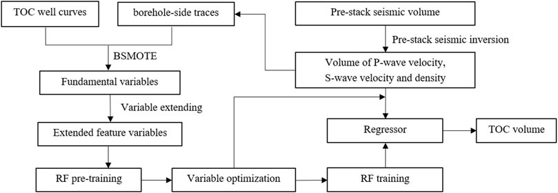
FIGURE 1. Workflow of the proposed approach.

2.1 Feature variables extension

The principles of classification and regression for RF are basically the same, with the difference being that classification outputs categorical labels and regression outputs numerical variables. For the classification problem, the prediction of RF is decided by a minority-majority voting method. For the regression problem, the average of all the regression decision tree output values is used as the prediction of the forest. Previous work in geophysics has shown that for RF classification, such as lithology and fluid identification, using several target-sensitive elastic properties obtained by pre-stack seismic inversion as input feature variables can yield good classification results (Kim et al., 2018; Lubo-Robles et al., 2022). However, for the regression of continuous numerical variable such as TOC, the influence of the number of elastic properties on the prediction results is not clear enough.

In general, the greater the number of feature variables involved in training, the richer the information carried will be and the training results may be more accurate and generalized. Alvarez et al. (2015) mathematically transformed 11 common elastic properties to obtain a large number of extended elastic properties as the base dataset for linear regression of petrophysical properties, which can achieve better application results. However, this approach is still influenced by subjective factors, e.g., the number of common elastic properties is much more than 11 and the target-sensitive elastic properties might be missed. In addition, the extraction of a large number of target-sensitive elastic properties is a time-consuming and expert-knowledge-requiring. Each elastic property needs to be obtained based on pre-stack seismic inversion or different transformation formulas, which is less automated and has the risk of error accumulation and amplification during the transformation process, especially for unconventional reservoirs whose elastic properties are anisotropic. To overcome the problems in the preparation of feature variables for RF training, we propose to automatically generate a series of elastic properties as feature variables using extended elastic impedance (EEI).

Whitcombe et al. (2002) proposed the expression of EEI based on the Connolly’s elastic impedance equation:

$\mathrm{E}\mathrm{E}\mathrm{I}\left(\chi \right)=V_{p_0}{\rho }_0\left[{\left(\frac{V_p}{V_{P_0}}\right)}^p{\left(\frac{V_s}{V_{s_0}}\right)}^q{\left(\frac{\rho }{{\rho }_0}\right)}^r\right](1)$

where $p=\left(\cos \chi +\sin \chi \right)$, $q=-8k\sin \chi$, $r=\left(\cos \chi -4k\sin \chi \right)$; $\chi$ represents the angle value that varies between −90°and +90°; $V_p$, $V_s$ and $\rho$ represent the P-wave velocity, S-wave velocity and density, respectively; $V_{p_0}$, $V_{s_0}$ and ${\rho }_0$ represent the mean values of P-wave velocity, S-wave velocity and density of the target layer, respectively.

In Eq. 1, the EEI is calculated from the three fundamental elastic properties: $V_p$, $V_s$ and $\rho$. The EEI is tuned using different $\chi$ values to be approximately proportional to a number of elastic properties for lithology or fluid identification (Whitcombe et al., 2002). Moreover, the EEI provides a good approximation of common logging properties (e.g., resistivity, gamma) (Neves, 2004). It is easy to obtain these fundamental elastic properties volumes through pre-stack seismic inversion technology (Russell et al., 2011; Yuan et al., 2019). We proposed to use EEI at different $\chi$ to replace the common elastic properties as the feature variables. Firstly, since there are some errors in the elastic properties obtained from the prestack seismic inversion, we use the noisy elastic properties for training to directly establish the relationship between the noisy properties and TOC, instead of considering the effect of errors separately. The borehole-side traces are extracted from the prestack seismic inversion volumes of $V_p$, $V_s$ and $\rho$ as the fundamental curves. The mean value $V_{p_0}$, $V_{s_0}$ and ${\rho }_0$ of the target layer can be statistically obtained from the fundamental curves. Since they only serve to standardize the magnitude of EEI with different angles, the correctness of their values does not affect the sensitivity of the EEI. Secondly, a series of EEI curves at different $\chi$ are calculated according to Eq. 1. In this study, we set the change step of $\chi$ to 5° (the step can be set smaller in order not to miss the potential target-sensitive elastic properties). Thirdly, 222 feature variables are extended according to the mathematical transformation ideal of Alvarez et al. (2015), as shown in Table 1. Theoretically, other mathematical operations can also be used for transformation and may yield better results, which can be set according to specific conditions. Finally, the extended feature variable traces and the corresponding TOC logging curves are used as the training set.

TABLE 1

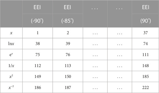
TABLE 1. Feature variables. x represents the angle-dependent extended elastic impedance. Each number represents a single variable, which is obtained after applying the mathematical operation shown in the leftmost column to the variable show in the uppermost row.

2.2 Performing balanced sampling

The original training set is resampled using the Bootstrap sampling to randomly generate k sub-training sets $S_1,S_2,\dots ,S_k$ (Breiman, 2001). The elements included in each sub-training set sampled by Bootstrap sampling are not all the same, ensuring the diversity of the decision tree, which is one of the advantages of the RF. However, all samples are sampled with the same probability each time in Bootstrap sampling process, which means that when training on sample sets with widely different numbers of samples from different classes, the results is often biased toward the majority class samples, and the minority class samples cannot obtain the desired results. In the past few years, the problem of classifying imbalanced data in machine learning has received increasing attention (Zhang et al., 2018). Here, “imbalanced data” means that the number of samples corresponding to each class is different and the number of differences is large. Although the imbalanced data problem is mainly focused on classification, its impact on regression cannot be ignored. For shale gas in southwest China, the “sweet spot” layer is usually thinly developed in large sets of shale. When the number of training samples belong to the “sweet spot” layers with higher TOC is small and the number of training samples belong to the non-“sweet spot” layers with lower TOC is large, the training of RF regressor may be biased to the non-“sweet spot” layers, which may affect the accuracy of TOC prediction in the “sweet spot” layers. The number of samples belong to “sweet spot” layers and non-“sweet spot” layers are needed to be balanced, forming a large balanced dataset.

There are two general methods for handling imbalanced data: oversampling and undersampling. Oversampling is to increase the size of a minority class sample by replicating a minority class sample. Undersampling, on the other hand, removes some majority class samples at random. Considering that machine learning relies mainly on logging data as training samples, which are expensive to obtain and often precious in small quantities. Therefore, we suggest the oversampling method is used to deal with the minority class samples. A more representative oversampling technique is the Synthetic Minority Oversampling Technique (SMOTE). The SMOTE algorithm analyzes a small number of samples, synthesizes new samples manually, and adds the new samples to the dataset. The specific procedure of this algorithm is as follows (Chawla et al., 2002):

(1) For each sample in the minority class (“sweet spot” layers with high TOC), we calculate its distance from all the samples in the minority set by using the Eucli-dean distance and obtain its m nearest neighbors;

(2) According to the imbalance class ratio, we set sampling ratio to determine the sampling magnification N. For sample x in the minority class, we randomly select several samples from its m nearest neighbors. For each randomly selected neighbor y, we construct a new sample z with the original sample x according to the equation:

$z=x+rand\left(\mathrm{0,1}\right)\times \left|y-x\right|(2)$

where $rand\left(\mathrm{0,1}\right)$ represents the random number between 0 and 1;

(3) Repeat steps (1)-(2) until the number of samples in the minority set increases to the pre-set value N.

The SMOTE algorithm may cause overlap between samples, generate some samples that do not provide effective information, and reduce the classification/regression performance. To further improve the generalization of the RF regressor for TOC prediction, we used the Borderline Synthetic Minority Oversampling Technique (BSMOTE) (Han et al., 2005) to take oversampling, which was improved based on the SMOTE. The BSMOTE algorithm only uses a minority of samples on the border to synthesize new samples, thereby improving the category distribution of the samples. The oversampling process of BSMOTE is basically the same as SMOTE, with the difference being that the BSMOTE further categorizes the minority samples into three categories: “Safe”, “Danger” and “Noise”. “Safe” category means that more than half of the samples are minority samples; “Danger” category means that more than half of the samples are majority samples, which are regarded as samples on the boundary; “Noise” category means that the samples are surrounded by the majority samples, which are regarded as noise. Finally, only the minority samples denoted as “Danger” are oversampled (Liu and Liu, 2022).

2.3 Optimal predictor training

RF is a bagging ensemble of many uncorrelated decision trees. The CART algorithm is applied to sub-training set $S_1,S_2,\dots ,S_k$ separately for decision tree modeling (Breiman, 2001). The partition criterion in CART for regression is the minimum mean squared error which is used to choose the feature for node partition. For each partition, the input space is split into two subspaces. After fully grown, the decision trees are constructed. Even with the same training samples, the features corresponding to each node on the decision tree are different due to the random selection of features, which makes the decision tree more diverse and improves the performance of the whole forest. Each decision tree can give a predicted TOC value, and the average of the predicted values of all k decision trees is used as the output value of TOC.

According to the proposed feature variable expansion method, 222 feature variables can be generated from the $V_p$, $V_s$ and $\rho$ volumes inverted by pre-stack seismic as the input data for the RF predictor. However, a large number of feature variables may bring too much redundant information and calculation consumption. Some feature variables may be extremely sensitive to TOC, while others may contain little valid information. Selecting the feature variables that contribute most to the target regression can speed up the process and improve the accuracy of prediction. Another advantage of RF is that it can provide a variable importance measure (VIM), which ranks feature variables according to their predictive power. In RF, there are Gini importance and permutation accuracy importance (Strobl et al., 2007). For regression problems like TOC, it is appropriate to use permutation accuracy importance to calculate the VIM. For Bootstrap sampling, each decision tree has its own out-of-bag samples, which are not used in the construction process. For Bootstrap sampling, each decision tree has its own out-of-bag data samples that are not used in the tree construction process and can be used to calculate the VIM.

There are three main steps in the VIM calculation of permutation accuracy importance. First, the predictive accuracy of the out-of-bag sample is measured. Second, the feature variables were randomly permuted, and the other feature variables were left unchanged. Finally, the prediction accuracy after random permutation is measured. For the ith tree, the VIM of the jth feature variable X_j is:

$V_{ij}=\frac{1}{K_{oob}}{{\sum }_{i=1}^{k_{oob}}\left(y_i-{\stackrel{\sim }{y}}_i\left(X_j\right)\right)}^2-\frac{1}{K_{oob}}{{\sum }_{i=1}^{k_{oob}}\left(y_i-{\stackrel{\sim }{y}}_i\right)}^2(3)$

where $K_{oob}$ is the number of out-of-bag samples, $y_i$ is the actual value, ${\stackrel{\sim }{y}}_i$ is the predicted value, and ${\stackrel{\sim }{y}}_i\left(X_j\right)$ is the predicted value of variable X_j after random permutation.

The average VIM of all trees is taken as the final VIM of X_j. Based on the VIM, the top-ranked feature variables are preferred as the final input feature variables for RF predictor training.

3 Examples

A shale gas reservoir study area in Southwest China is used as an example to discuss the effectiveness of the new method. The shale in this study area is buried deep (>3,500 m) and widely distributed with large thickness. The early deployed exploratory wells obtained high production gas flow, showing the huge resource potential of deep shale gas in the area. However, as more exploratory wells are deployed, significant lateral changes in production capacity have been observed, resulting in significant exploration risks. Therefore, the spatial distribution of high-quality “sweet spot” needs to be finely delineated. Drilling data show that the high quality “sweet spot” layer in this study area has high TOC with various types of pore space including inorganic mineral and organic pores. The relationship between TOC and elastic properties is affected by the complex lithofacies and pore structures, as well as temperature and pressure, which makes it difficult to accurately establish rock-physics models, resulting in low inversion accuracy of TOC based on model driven methods. Therefore, it is necessary to try to obtain high accuracy TOC distribution information based on data-driven approach.

Figure 2 shows the borehole-side curves extracted from the prestack seismic inversion volumes of $V_p$, $V_s$ and $\rho$, and the corresponding TOC well logging interpretation curve of a key well in this study area. We can observe that TOC curve is not directly related to curves of $V_p$, $V_s$ and $\rho$. Figure 3 shows the EEI curves of different angles and Lamé impedance (λρ) curve calculated by $V_p$, $V_s$ and $\rho$ shown in Figure 2. The result of λρ is commonly used as an properties that responds to changes in rock rigidity or an indicator of fluid identification (Goodway et al., 1997). We observe that there are some differences between the EEI curves with different angles. When the angle is 15°, EEI (15°) is very similar to the λρ curve, with a Pearson correlation coefficient of 0.98, which indicates that the EEI can be indeed used as a substitute for some common elastic properties.

FIGURE 2

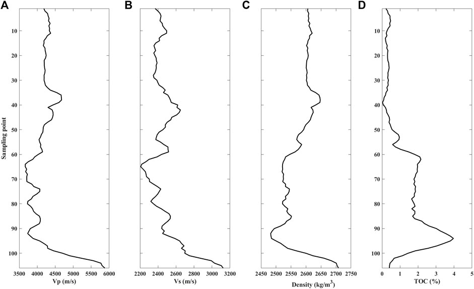
FIGURE 2. Well logging curves. (A) P-wave velocity, (B) S-wave velocity, (C) density, (D) TOC.

FIGURE 3

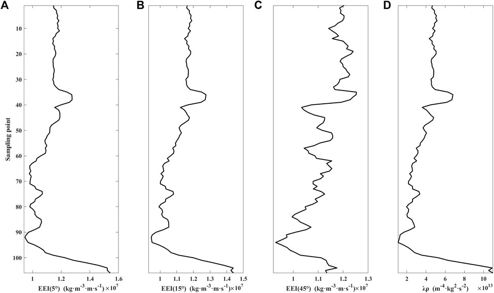
FIGURE 3. Elastic properties curves. (A) EEI (5°), (B) EEI (15°), (C) EEI (45°), (D) λρ.

As for which feature variable is more important it still has to be selected based on the specific study area and the VIM ranking. According to the generation way shown in Table 1, 222 extended variables are obtained for VIM ranking as shown in Figure 4. For this case, we observe that not every variable is important for TOC prediction, and the 206th variable ($\mathrm{E}\mathrm{E}\mathrm{I}{\left(10°\right)}^{-2}$) has the highest importance. The curves of the highest importance variable and the lowest importance variable ($\mathrm{E}\mathrm{E}\mathrm{I}{\left(80°\right)}^2$) is shown in the Figure 5. We can see that the trend of the highest importance variable can roughly reflect the change of TOC curve, while the trend of the lowest importance variable looks unrelated to the TOC curve. With this extension strategy, not all common elastic properties can be covered, but potential TOC-sensitive parameters can be obtained unconsciously.

FIGURE 4

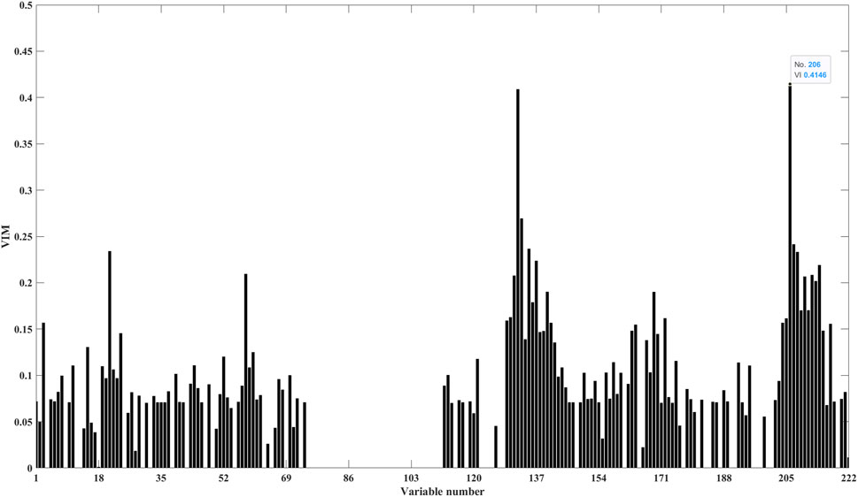
FIGURE 4. VIM of feature variables.

FIGURE 5

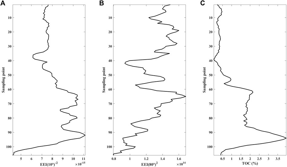
FIGURE 5. Curves comparison. (A) Variable with highest VIM, (B) Variable with highest VIM, (C) TOC.

From Figure 4, we also can see that many variables have very low VIM, which indicates the existence of information redundancy. The variables are added to the RF training sequentially according to the ranking from highest to lowest VIM, and changes in corresponding Pearson correlation coefficient between the predicted TOC curve and the true TOC curve with the number of variables are shown in Figure 6. We observe that the Pearson correlation coefficient shows an upward trend with the increase of the number of feature variables, and then tends to be flat when the number reaches about 40. Therefore, we conclude that in this example, only the VIM top 40 feature variables are required to meet the requirements.

FIGURE 6

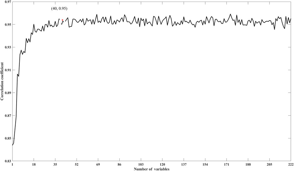
FIGURE 6. Pearson correlation coefficient changes with the number of feature variables.

Figure 7 shows the TOC curves predicted using all 222 variables, only the VIM top 40 variables and 11 common elastic properties (P-wave impedance, S-wave impedance, P-to-S velocity ratio, density*Lamé’s parameters and subtraction of the two, density*shear modulus, Poisson’s ratio, density*Young’s modulus, density*bulk modulus, Poisson dampening factor) as the input feature variables. We see that the predicted curves of all 222 variables and the VIM top 40 variables are almost coincident on the whole, which are both better than the predicted result of the common 11 elastic properties. However, in Figure 7, we also observe that even the prediction result of 222 variables deviates significantly in the high TOC interval (as shown by the arrow). Our analysis suggests that the proportion of high TOC intervals in the entire curve is relative very small, resulting in the training of the RF regressor leaning towards low TOC samples. As shown in the histogram in Figure 8, the high TOC samples accounts for a small proportion in the whole sample set. Therefore, it is necessary to balance the samples participating in the training. We used BSMOTE to increase the number of samples in the high TOC interval. As shown in Figure 9, it can be seen that after BSMOTE processing, the number of samples with low TOC in the original sample did not change, while the number of samples with high TOC significantly increased and the values were more diverse. The number of samples with high and low TOC reached a rough balance. The prediction result of the VIM top 40 variables after BSMOTE processing is shown in Figure 10. By comparing Figure 7 and Figure 10, it can be observed that the prediction results for high TOC intervals are significantly improved, with the correlation coefficient increasing to 0.98 from the previous 0.95, which indicates that the issue of sample balance cannot be ignored for the RF prediction of imbalanced data. Figure 11 shows the predicted TOC of another well in the study area that did not participate in training as a blind well. It can be seen that although this well did not participate in the training, the prediction result is still in good agreement with the logging curve, with a correlation coefficient of 0.96, which also verifies the effectiveness of the proposed method.

FIGURE 7

FIGURE 7. Comparison of prediction curves. The black, green, blue, and red curves represent the real TOC well logging interpretation curve, predicted curve by the common 11 elastic properties and predicted curve by the all 222 feature variables, predicted curve by the VIM top 40 feature variables, respectively.

FIGURE 8

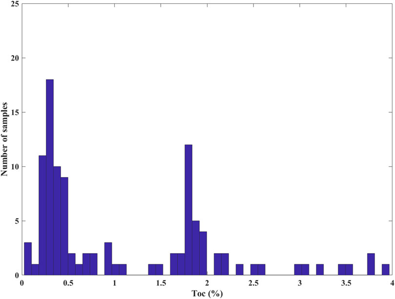
FIGURE 8. Histogram of TOC before BSMOTE processing.

FIGURE 9

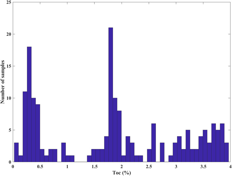
FIGURE 9. Histogram of TOC after BSMOTE processing.

FIGURE 10

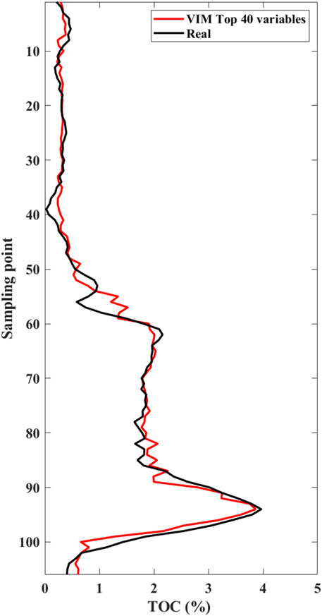
FIGURE 10. Comparison of prediction curves. The black and red curves represent the real TOC well logging interpretation curve and the predicted curve by the VIM top 40 feature variables, respectively.

FIGURE 11

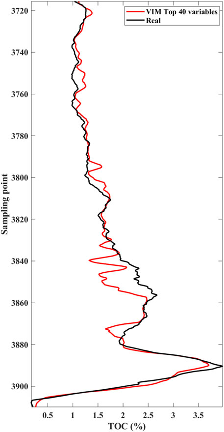
FIGURE 11. Comparison of prediction curves of a validation well. The black and red curves represent the real TOC well logging interpretation curve and the predicted curve by the proposed approach.

The seismic data in this area have been rigorously processed and quality controlled to meet the requirements for pre-stack seismic inversion. Figure 12 show a pre-stack seismic inversion section of three fundamental elastic properties in the target area. From the values presented by the P-wave velocity, S-wave velocity, and density sections, there is no intuitive and unified pattern to help us identify favorable “sweet spots”. Further conversion of the elastic properties to TOC is required. Based on three fundamental elastic properties, the TOC section was predicted using the common 11 elastic properties and VIM top 40 variables after BSMOTE processing as input feature variables, respectively, as shown in Figure 13. It can be observed that there is a significant difference in the relative high TOC development area predicted by the common method and the proposed approach (shown by the red dashed lines). The relative high TOC (about 4.2%) development interval predicted by the proposed approach is below the relative high TOC development interval predicted by the common method, which has obvious anomaly and good continuity compared with the surrounding strata. Subsequent horizontal drilling confirmed the development of a continuous high-quality shale gas reservoir in this layer with TOC averaging around 4%, which verifies the effectiveness of the proposed method. Although the results of common method also exhibit locally high TOC values (about 3.5%) in this interval (shown by the red arrow), the continuity is poor and can easily be misinterpreted as a reservoir with low commercial exploration value.

FIGURE 12

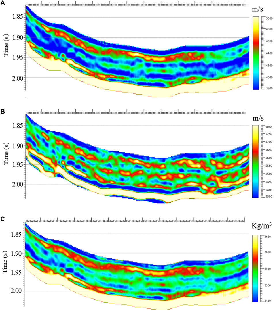
FIGURE 12. Elastic properties section. (A) P-wave velocity, (B) S-wave velocity, (C)Density.

FIGURE 13

FIGURE 13. Comparison of TOC prediction sections. (A) Predicted by the common 11 elastic properties, (B) Predicted by the proposed approach.

4 Conclusion

In gas reservoir research areas with complex geological environments or lack of rock-physics experimental analysis data, it is difficult to accurately establish rock-physics models between petrophysical properties and seismic or their derived elastic properties, resulting in insufficient theoretical basis for model-driven approaches. Data-driven approaches, with their powerful ability to uncover the complex statistical relationship by learning a favorable predictor, provide a new way to break this situation. For continuous numerical regression problems such as TOC, data-driven approaches require a large number of feature variables as training sets in order to achieve the best performance. However, extracting valid feature variables from seismic data is a very tedious and experience-dependent task. In addition, for the describing of thin reservoirs developed in a large set of background lithology, the issue of imbalanced samples cannot be ignored. To address the challenges of data-driven approach in the application of TOC prediction, we first propose to use extended elastic impedance to automatically generate 222 extended elastic properties as the training set for machine learning, and introduce the RF algorithm to optimize the training of the regressor. Then, taking the advantage that RF can rank the importance of feature variables, the feature variables with higher importance for TOC prediction are preferentially selected to participate in the final training to reduce the redundancy of information. The BSMOTE is used to improve the problem of RF training with imbalanced samples. Both the analysis of well-logging data and the field data application demonstrate the superiority and validity of the proposed method for TOC prediction. Furthermore, the applications of the proposed method are not limited to predict TOC. It also can be easily extended to perform predictions of other petrophysical properties such as porosity, gas content and even stress, brittleness, etc. In addition, the proposed method is also suitable for other machine learning algorithms. Because preparing sufficient feature variables is the primary problem faced by all supervised machine learning algorithms for geophysical applications and the problem of data imbalance is very common in the field of geophysics.

Data availability statement

The original contributions presented in the study are included in the article/Supplementary Material, further inquiries can be directed to the corresponding author.

Author contributions

JiG, JaG, and SL contributed to conception and design of the study. HL organized the database. BL performed the statistical analysis. JiG wrote the first draft of the manuscript. All authors contributed to the article and approved the submitted version.

Funding

This work was supported by the Forward-looking and Fundamental Science and Technology Research Projects of PetroChina (2021DJ0606), the Basic Research and Strategic Reserve Technology Research Fund Project of Research Institutes Directly under Petrochina (2022D-XB01).

Acknowledgments

The authors would like to thank the editors and reviewers for their valuable suggestions for this paper.

Conflict of interest

Authors JiG, JaG, SL, HL, BL, and XG were empolyed by PetroChina.

Publisher’s note

All claims expressed in this article are solely those of the authors and do not necessarily represent those of their affiliated organizations, or those of the publisher, the editors and the reviewers. Any product that may be evaluated in this article, or claim that may be made by its manufacturer, is not guaranteed or endorsed by the publisher.

References

Alvarez, P. K., and Bolivar, F. A. (2015). Multi-attribute rotation scheme—a new tool for reservoir properties prediction from seismic inversion attributes. Interpretation 3 (4), SAE9–SAE18. doi:10.1190/INT-2015-0029.1

CrossRef Full Text | Google Scholar

Amosu, A., and Sun, Y. (2019). “Effective machine learning approach for identifying high total organic carbon formations,” in SEG technical program expanded abstracts 2019 (Houston: Society of Exploration Geophysicists), 2363–2367. doi:10.1190/segam2019-3215229.1

CrossRef Full Text | Google Scholar

Bandura, L., Halpert, A. D., and Zhang, Z. (2018). “Machine learning in the interpreter’s toolbox: unsupervised, supervised, and deep-learning applications,” in SEG technical program expanded abstracts 2018 (Houston: Society of Exploration Geophysicists), 4633–4637. doi:10.1190/segam2018-2997015.1

CrossRef Full Text | Google Scholar

Bandyopadhyay, K., Sain, R., Liu, E., Harris, C., Martinez, A., Payne, M., et al. (2012). “Rock property inversion in organic-rich shale: uncertainties, ambiguities, and pitfalls,” in 2012 SEG annual meeting (Houston: Society of Exploration Geophysicists). doi:10.1190/segam2012-0932.1

CrossRef Full Text | Google Scholar

Breiman, L., Friedman, H., Olshen, A., Olshen, R. A., and Stone, C. J. (1984). Classification and regression trees. Biometrics 40 (3), 874. doi:10.2307/2530946

CrossRef Full Text | Google Scholar

Breiman, L. (2001). Random forests. Mach. Learn. 45 (1), 5–32. doi:10.1023/A:1010933404324

CrossRef Full Text | Google Scholar

Chawla, N. V., Bowyer, K. W., Hall, L. O., and Kegelmeyer, W. P. (2002). Smote: synthetic minority over-sampling technique. J. Artif. Intell. Res. 16, 321–357. doi:10.1613/jair.953

CrossRef Full Text | Google Scholar

Chopra, S., Sharma, R. K., and Marfurt, K. J. (2010). “Current workflows for shale gas reservoir characterization,” in SEG global meeting abstracts. (Houston: Society of Exploration Geophysicists), 1905–1910. doi:10.1190/urtec2013-194

CrossRef Full Text | Google Scholar

Cracknell, M. J., and Reading, A. M. (2014). Geological mapping using remote sensing data: A comparison of five machine learning algorithms, their response to variations in the spatial distribution of training data and the use of explicit spatial information. Comput. Geosciences 63, 22–33. doi:10.1016/j.cageo.2013.10.008

CrossRef Full Text | Google Scholar

Goodway, B., Chen, T., and Downton, J. (1997). “" Improved AVO fluid detection and lithology discrimination using Lamé petrophysical parameters; “λρ”,“μρ”,&“λ/μ fluid stack”, from P and S inversions,” in SEG technical program expanded abstracts 1997 (Houston: Society of Exploration Geophysicists), 183–186. doi:10.1190/1.1885795

CrossRef Full Text | Google Scholar

Grana, D., Azevedo, L., Figueiredo, L. d., Connolly, P., and Mukerji, T. (2022). Probabilistic inversion of seismic data for reservoir petrophysical characterization: review and examples. Geophysics 87 (5), M199–M216. doi:10.1190/geo2021-0776.1

CrossRef Full Text | Google Scholar

Gui, J., Gao, J., Yong, X., Li, S., Liu, B., and Zhao, W. (2015). Reservoir parameter inversion based on weighted statistics. Appl. Geophys. 12 (004), 523–532. doi:10.1007/s11770-015-0523-z

CrossRef Full Text | Google Scholar

Han, H., Wang, W. Y., and Mao, B. H. (2005). “Borderline-SMOTE: A new over-sampling method in imbalanced data sets learning,” in Advances in intelligent computing. ICIC 2005. Lecture notes in computer science (Berlin, Heidelberg: Springer). doi:10.1007/11538059_91

CrossRef Full Text | Google Scholar

Jiang, L., Castagna, J. P., Russell, B., and Guillen, P. (2020). “Rock physics modeling using machine learning,” in SEG technical program expanded abstracts 2020 (Houston: Society of Exploration Geophysicists), 2530–2534. doi:10.1190/segam2020-3427097.1

CrossRef Full Text | Google Scholar

Kim, Y., Hardisty, R., Torres, E., and Marfurt, K. J. (2018). “Seismic-facies classification using random forest algorithm,” in SEG technical program expanded abstracts 2018 (Houston: Society of Exploration Geophysicists), 2161–2165. doi:10.1190/segam2018-2998553.1

CrossRef Full Text | Google Scholar

Kumar, R., Bansal, P., Al-Mal, B. S., Dasgupta, S., Sayers, C. M., Ng, P. H. D., et al. (2016). “Orthotropic rock-physics based inversion for fracture and total organic carbon (TOC) characterization from azimuthal P-wave seismic survey: case study from a northern Kuwait unconventional reservoir,” in SEG Technical Program Expanded Abstracts 2016 (Houston: Society of Exploration Geophysicists), 3210–3215. doi:10.1190/segam2016-13685275.1

CrossRef Full Text | Google Scholar

Li, M. X., Han, H. W., Liu, H. J., Sang, W. J., and Yuan, S. Y. (2023). Permeability prediction and uncertainty quantification base on Bayesian neural network and data distribution domain transformation. Chin. J. Geophys. 66 (4), 1664–1680. (in Chinese). doi:10.6038/cjg2022P0837

CrossRef Full Text | Google Scholar

Liu, J., and Liu, J. (2022). Integrating deep learning and logging data analytics for lithofacies classification and 3D modeling of tight sandstone reservoirs. Geosci. Front. 13 (1), 101311. doi:10.1016/j.gsf.2021.101311

CrossRef Full Text | Google Scholar

Lubo-Robles, D., Devegowda, D., Jayaram, V., Bedle, H., Marfurt, K. J., and Pranter, M. J. (2022). Quantifying the sensitivity of seismic facies classification to seismic attribute selection: an explainable machine-learning study. Interpretation 10 (3), SE41–SE69. doi:10.1190/INT-2021-0173.1

CrossRef Full Text | Google Scholar

Neves, F. A., Mustafa, H. M., and Rutty, P. M. (2004). Pseudo-gamma ray volume from extended elastic impedance inversion for gas exploration. The Leading Edge 23 (6), 536–540. doi:10.3997/2214-4609-pdb.3.D007

CrossRef Full Text | Google Scholar

Ouadfeul, S.-A., and Aliouane, L. (2016). Total organic carbon estimation in shale-gas reservoirs using seismic genetic inversion with an example from the Barnett Shale. Lead. Edge 35 (9), 790–794. doi:10.1190/tle35090790.1

CrossRef Full Text | Google Scholar

Pedro, A., Francisco, B., Mario, D., and Salinas, T. (2015). Multiattribute rotation scheme: A tool for reservoir property prediction from seismic inversion attributes. Interpretation 3 (4), SAE9–SAE18. doi:10.1190/INT-2015-0029.1

CrossRef Full Text | Google Scholar

Russell, B. H., Gray, D., and Hampson, D. P. (2011). Linearized AVO and poroelasticity. Geophysics 76 (3), C19–C29. doi:10.1190/1.3555082

CrossRef Full Text | Google Scholar

Sachsenhofer, R. F., Leitner, B., Linzer, H.-G., Bechtel, A., Ćorić, S., Gratzer, R., et al. (2010). Deposition, erosion and hydrocarbon source potential of the oligocene Eggerding formation (molasse basin, Austria). Austrian J. Earth Sci. 103 (1), 76–99.

Google Scholar

Sang, W. J., Yuan, S. Y., Han, H. W., Liu, H. J., and Yu, Y. (2023). Porosity prediction using semi-supervised learning with biased well log data for improving estimation accuracy and reducing prediction uncertainty. Geophys. J. Int. 232 (2), 940–957. doi:10.1093/gji/ggac371

CrossRef Full Text | Google Scholar

Sondergeld, C. H., Newsham, K. E., Comisky, J. T., Rice, M. C., and Rai, C. S. (2010). “Petrophysical considerations in evaluating and producing shale gas resources,” in SPE unconventional gas conference. Pennsylvania: SPE. doi:10.2118/131768-MS

CrossRef Full Text | Google Scholar

Strobl, C., Boulesteix, A.-L., Zeileis, A., and Hothorn, T. (2007). Bias in random forest variable importance measures: illustrations, sources and a solution. BMC Bioinforma. 8 (1), 25–21. doi:10.1186/1471-2105-8-25

PubMed Abstract | CrossRef Full Text | Google Scholar

Verma, S., Zhao, T., Marfurt, K. J., and Devegowda, D. (2016). Estimation of total organic carbon and brittleness volume. Interpretation 4 (3), T373–T385. doi:10.1190/int-2015-0166.1

CrossRef Full Text | Google Scholar

Whitcombe, D. N., Connolly, P. A., Reagan, R. L., and Redshaw, T. C. (2002). Extended elastic impedance for fluid and lithology prediction. Geophysics 67 (1), 63–67. doi:10.1190/1.1451337

CrossRef Full Text | Google Scholar

Wilson, T., Kavousi, P., Carr, T., Carney, B., Uschner, N., Magbagbeola, O., et al. (2017). “Relationships of λρ, µρ, brittleness index, Young's modulus, Poisson's ratio, and high total organic carbon for the Marcellus Shale, Morgantown, West Virginia,” in SEG International Exposition and Annual Meeting 2017 (Houston: Society of Exploration Geophysicists), 3438–3442. doi:10.1190/segam2017-17631837.1

CrossRef Full Text | Google Scholar

Yin, J., Gao, C., Cheng, M., Liang, Q., Xue, P., Hao, S., et al. (2023). TOC interpretation of lithofacies-based categorical regression model: A case study of the yanchang formation shale in the ordos basin, NW China. Front. Earth Sci. 10. doi:10.3389/feart.2022.1106799

CrossRef Full Text | Google Scholar

Yu, Z., Ma, S., and Liu, C. (2023). TOC prediction and grading evaluation based on variable coefficient △logR method and its application for unconventional exploration targets in Songliao Basin. Front. Earth Sci. 11. doi:10.3389/feart.2023.1066155

CrossRef Full Text | Google Scholar

Yuan, S., Wei, W., Wang, D., Shi, P., and Wang, S. (2019). Goal-oriented inversion-based NMO correction using a convex l_2,1-norm. IEEE Geoscience Remote Sens. Lett. 17 (1), 162–166. doi:10.1109/LGRS.2019.2915520

CrossRef Full Text | Google Scholar

Zhang, G., Wang, Z., and Chen, Y. (2018). Deep learning for seismic lithology prediction. Geophys. J. Int. 215 (2), 1368–1387. doi:10.1093/gji/ggy344

CrossRef Full Text | Google Scholar

Zhao, L., Qin, X., Han, D.-H., Geng, J., Yang, Z., and Cao, H. (2016). Rock-physics modeling for the elastic properties of organic shale at different maturity stages. Geophysics 81 (5), D527–D541. doi:10.1190/geo2015-0713.1

CrossRef Full Text | Google Scholar