
95% of researchers rate our articles as excellent or good
Learn more about the work of our research integrity team to safeguard the quality of each article we publish.
Find out more
ORIGINAL RESEARCH article
Front. Earth Sci. , 29 August 2023
Sec. Geoscience and Society
Volume 11 - 2023 | https://doi.org/10.3389/feart.2023.1234732
 Shengting Ma*
 Shanshan Zhang
The concentrated connection of arable land is one of the important indicators reflecting the quality of cultivated land, and large-scale arable land blocks are more conducive to agricultural mechanization operation, thereby improving the land use efficiency. However, the calculation of farmland connectivity is essentially a large-scale calculation of spatial vector data, especially for the national or global farmland patch data. This article proposes a framework for calculating farmland connectivity based on spatial vector map tiles and parallelizes the algorithm based on the Hadoop cloud platform. The framework is based on the tile pyramid model and uses the Douglas–Peucker algorithm to simplify the data to meet the needs of rapid display of large-scale data under multi-scale. The consistency and integrity of the front display of vector tiles are ensured using the setting tile buffer. Meanwhile, the parallelization of the vector tile construction algorithm is realized based on the MapReduce programming mode. Finally, the effectiveness and usability of this framework were verified through the calculation of patch connectivity on the tillage map. Experiments show that the algorithm can not only meet the rapid construction requirements of large-scale vector tile data but also support the cultivated land spatial connectivity analysis and greatly improve the efficiency of supporting data calculation.
Since the State Council issued the Program of Action for the Development of Big Data in 2015, big data have been clearly identified as an important part of China’s basic strategic resources. The arrival of the era of big data not only makes people realize the importance of data but also triggers fundamental changes in many fields (Li and Li, 2014). Specifically, in the field of spatial information technology, how to solve the efficiency problem brought by big data has become an important research direction of many scholars (Jia et al., 2015; Yang et al., 2017). Among them, the rapid browsing and viewing of geographic information system (GIS) data has become an obstacle to large-scale data mining and analysis, such as patch connectivity and spatial overlay analyses (Ramos et al., 2009; Yao and Li, 2018), especially in the era of big data (Zouhar and Senner, 2019; Yao et al., 2023).
In agricultural land, the connectivity of cultivated land patches is one of the main indicators to measure the quality of cultivated land. The higher the connectivity, the greater the potential for the development and utilization of cultivated land and the more suitable it is for agricultural mechanization operations. However, the complexity of calculating the patch connectivity index of the cultivated map is often related to the number of patches, and the larger the data volume is, the more complex the calculation. The larger the amount of farmland plot data, the better the data rendering effect, and then, the traditional raster tile technology using static (fixed resolution) cache has been unable to meet the requirements of large-scale vector data multi-scene application (Guo et al., 2016; Wan et al., 2016). For example, map rendering should be carried out according to different field contents for different datasets such as the national map spot quality. Using raster tiles can only generate map tile sets several times, which not only multiplies the workload of data processing (Wang et al., 2022) but also brings a lot of map tile management and transmission costs. In addition, due to the deficiency of grid tiles, the data accuracy can only be displayed according to a fixed scale. Moreover, the data interaction is not flexible enough. The emergence of vector tile technology solves the aforementioned problems well.
Vector tile technology can be regarded as the product of the combination of raster tile and vector data (Yan et al., 2018). It adopts true vector data format to replace the raster picture format. In this way, it inherits mature map caching, hierarchical scaling, and other technologies in the raster tile model (Zhou et al., 2016). At the same time, the vector characteristics of the original data are preserved to the greatest extent. Through the map vector tile technology, the original vector data can be retrieved when the map is browsed under large scale or scaled at the bottom of the pyramid model. On this basis, the client can realize map dynamics, custom rendering, and symbolization, and also directly carry out vector data query and even spatial analysis and other complex operations (Huang et al., 2016). It greatly reduces the server access and computing pressure, and improves the performance and user experience of the WebGIS application system (Liu et al., 2022).
At present, there is no clear format standard and technical system standard for vector tile technology. Major commercial GIS development platforms, such as ArcGIS and SuperMap, also provide the construction function of the vector tile in the latest version. However, due to high software costs and commercial secrets, application cases and public technical information are relatively few. Some open source software, such as MapBox and GeoServer, also provide vector tile generation technology, but in the face of large-scale GIS vector data, there are still the following problems: 1) the production process of the map vector tile takes a long time or even cannot be completed; 2) the amount of spatial data that can be executed at one time is limited, so manual “divide and rule” is often used to increase the number of servers to complete the slicing task of large-scale vector data; and 3) the generated large-scale vector tiles cannot be acquired quickly, and the tile retrieval efficiency is low. In recent years, cloud computing technology has achieved good performance in processing spatial big data and also provides effective solutions for the storage, management, and analysis of vector big data (Yang et al., 2013; Li et al., 2016). Cloud computing technology is relatively mature in algorithms and applications to improve the construction performance of raster tiles. For example, SpatialHadoop (Eldawy and Mokbel, 2015; Alarabi et al., 2018) conducted a batch construction study of raster tiles for large-scale remote sensing images based on the MapReduce programming model. LandQv2 (Yao et al., 2018a) realized the design and implementation of the raster tile pyramid algorithm for vector data based on the Hadoop cloud platform, which met the requirements for rapid visualization of national map spot quality and other data. In the aspect of vector tile construction, the basic idea framework is similar to the parallelization of raster tiles. However, due to the different sizes and shapes of vector elements, the algorithm is more complex (Yao et al., 2018b). It is not only necessary to consider the pyramid model longitudinal data simplification or thinning algorithm but also to consider the cutting and unification of horizontal pattern patch elements.
In this paper, the application of map vector tiles meets the demand of rapid display of large-scale data in the multilevel scale. The Douglas–Peucker simplified algorithm was used to compress data, and the tile buffer was set to ensure the consistency and integrity of the front display of the vector tile. Based on the MapReduce programming model, the parallel construction algorithm of the vector tile is implemented and tested. Finally, the effectiveness and usability of this framework were verified through the calculation of patch connectivity on national tillage maps, and good results are obtained.
The tile pyramid model is a kind of multi-resolution hierarchical model; in a linear quadtree structure tile (Figure 1), the maximum number of tile n layer of 22n; with the increase in the hierarchy, the resolution increases. The vector tile and grid tile have the same pyramid model, and the method of cutting is the same (Yan et al., 2018). Different map manufacturers adopt different map tile cutting algorithms; this paper uses the OpenStreetMap tile segmentation method. The formula is expressed as follows:
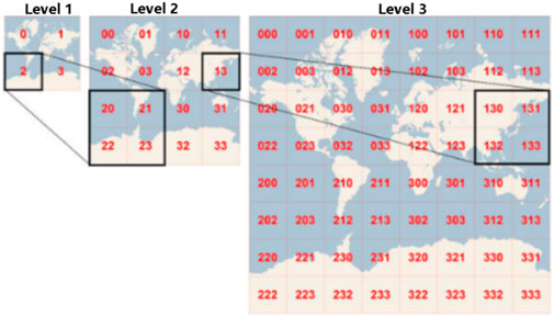
FIGURE 1. Tile pyramid model (Yan et al., 2018).
Inverse operation is represented as follows:
where lon and lat are the latitude and longitude, respectively, and x and y are the column numbers of the tile at the z level. With the upper left corner of the map as the origin, according to the map from left to right, from top to bottom in order to divide into grids, according to the formula to calculate the ranks of each layer of each tile, that is, the tile’s unique index number.
In the Web map request map tiles, according to the tile number index, only the request display range of tiles, which reduces the unnecessary network transmission consumption, also reduces the pressure of graphics rendering.
In map, in order to realize the rapid display of map elements under a small scale, vector data are generally compressed and simplified to reduce the amount of data. The Douglas–Peucker algorithm is a classical vector data compression algorithm, which has the advantages of translation, rotation invariability, and consistent sampling results (Yao et al., 2018b), but the disadvantage is that the topological relationship cannot be maintained. The Java Topology Suite (JTS) library implements the Douglas–Peucker algorithm, which can simplify vector data well and quickly.
The Douglas–Peucker algorithm simplifies the process described as follows (Figure 2): 1) find the two endpoints of the curve and connect them in a straight line; 2) calculate the distance between other points and this line, and find the point with the maximum distance; 3) determine the size of the maximum distance and the given tolerance. If less than the tolerance, then discard; if it is greater than the tolerance, keep the point and divide the curve into two parts, and repeat the aforementioned steps recursively for these two parts; and 4) after the completion of recursion, connect the retained points to obtain the simplified curve. For the surface element, it is first converted to the line element and then simplified.
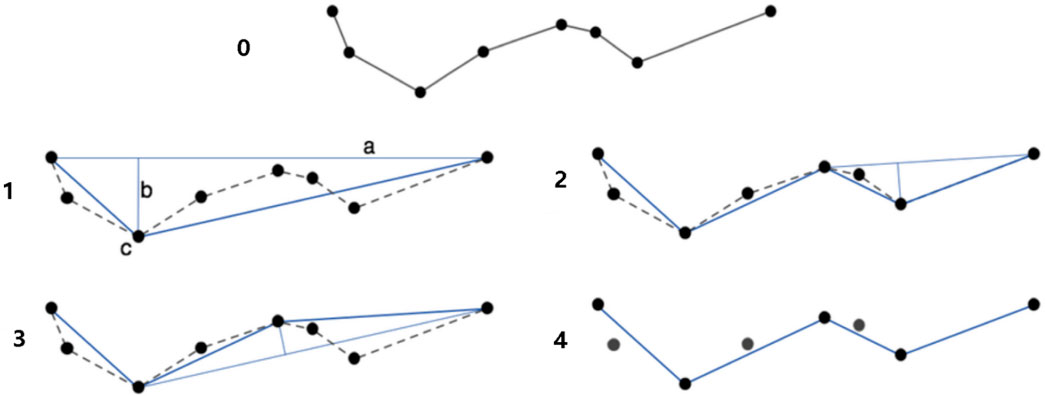
FIGURE 2. Simplified process of the Douglas–Peucker algorithm (Yao et al., 2018b).
Vector tiles need to be concatenated on the front end of WebGIS to form a complete vector tile map, and after concatenation and visualization, grid lines of tiles may appear, leading to incomplete map display. This causes visual interference. This is because during the cutting of tiles and feature geometry, the two undergo an intersection operation, and the intersection result preserves the boundaries of the tiles. Therefore, tile splicing will display the boundary lines of the tiles.
Tile is actually a polygon grid. In the process of tile construction, the tile grid and space elements are intersected, and the boundary of the tile is retained as a result. In the display of splicing, the boundary is also drawn into the map, resulting in incomplete splicing of tile elements and affecting the appearance of the map, as shown in Figure 3A, specifically because there will be tile boundaries on the map. Some scholars have proposed methods to expand the tile cutting range based on Canvas technology, forming a buffer zone for tiles. When cutting, the tile cutting range is properly expanded to include excess elements. During the display, the browser only displays the elements inside the canvas and does not display the tiles outside the canvas, which ensures the complete splicing of tiles and elements and avoids the problem of tile boundary display, as shown in Figure 3B.
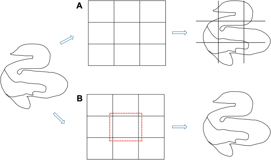
FIGURE 3. Tile extended buffer of the tile.
Common tile coding schemes include Geo JavaScript Object Notation (GeoJSON), MapBox Vector Tile (MVT), and other formats. The GeoJSON format is readable, and the front-end JavaScript supports the JSON data format natively, but the disadvantage is that the size of the GeoJSON data increases as the size of the data increases. The MVT format is MapBox based on a support multilingual, multi-platform, easy extension Protocol buffer Binary Format sequence of data format (PBF), which makes vector tiles coding format. When the amount of data is large, the decoding rate of PBF remains stable, while the decoding rate of JSON decreases with the increase in the amount of data. The decoding rate of the former is about 17 times that of the latter, and the compression rate is about two times (Yao et al., 2018a). Therefore, compared with the GeoJSON format, the PBF-based MVT format can compress data effectively, occupy less storage space, and consume less bandwidth for network transmission. At present, the underlying storage of the vector tile in GIS software applications such as ArcGIS, SuperMap, and GeoServer is the PBF format tile. In this paper, the MVT format is selected as the tile storage format.
As shown in Table 1, MVT coding standard geometry codes are the elements of space data serialization for the 32-bit unsigned integer, through three instructions MoveTo, LineTo, and ClosePath, and coordinate points (dX and dY) describe spatial location elements.
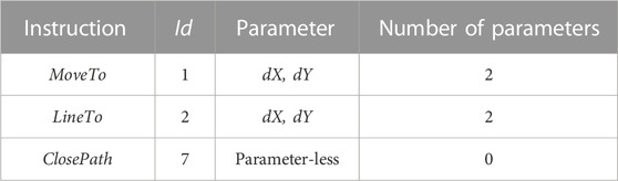
TABLE 1. Graphic coding instruction.
Command integer (Ci) was obtained by encoding the instruction id and the count of instruction execution:
Inverse operation is represented as follows:
Parameter value: the parameter integer (Pi) was obtained in the zigzag encoding mode. Parameter values of small negative or positive numbers were encoded into small integers to save storage space.
Parameter value: the value cannot be outside the range of
Pi decode is represented as follows:
Before encoding, the spatial elements need to be converted from geographic or projected coordinates to pixel coordinates of the screen. Point coordinates record the position of the next point in increments, which greatly compresses the amount of data. The encoding process is shown in Figure 4.
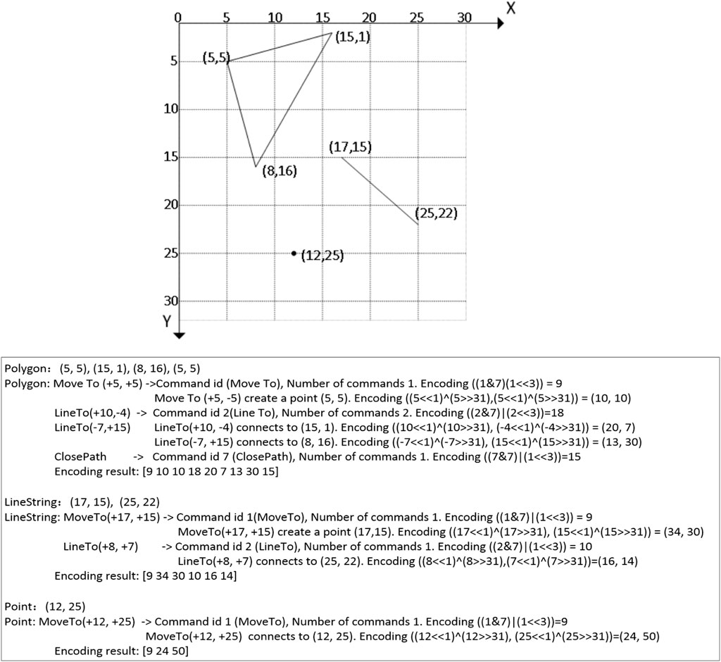
FIGURE 4. Geometric coding.
Each tile is a layer. In a layer, the attributes of all elements are stored in the form of key–value pairs. The key and value of all elements are indexed into the property name keys and values list, in which the index starts from 0. The attribute information on the element is expressed in pairs of integers in the tags field. Every two tags is a pair. The first integer represents the index number of key in the keys list, and the second integer represents the index number of value in the values list of the attribute value. All elements in the layer share the values in the two lists, and the same attribute name or attribute value of different elements will be indexed to the same key or value, thus avoiding duplicate data recording and reducing data redundancy. In addition, the geometry encoding result is stored in the geometry field.
Using MapReduce parallel computing, the parallel cutting of vector tiles is mainly divided into two stages: 1) parallel analysis of the Shapefile vector data set and 2) parallel construction of tiles.
Hadoop MapReduce is a classic example of the MapReduce parallel computing model. MapReduce is based on the Hadoop distributed file system (HDFS). After Hadoop2.0, the cluster resource management system, Yet Another Resource Negotiator (YARN), is added to coordinate the computing model with the scheduling of underlying storage and cluster resources to adapt to more computing models.
The general execution process of Hadoop MapReduce is described as follows:
(1) The input data are cut into data fragments.
(2) Data fragments are read into the Map in the form of key and value.
(3) After the data are passed into the Map function, the processing logic and flow are user-defined. After the Map processing is complete, it is still output as key and value. The input and output formats of key and value can also be user-defined.
(4) Data output in the Map phase enters the shuffle phase. Shuffle sorts and merges data. However, shuffle does not change the entered data. The format of the data is still Key2 and Value2. The values of the same keys are merged into the set Value2.
(5) After the shuffle is completed, data are transferred to the reduce phase for processing. The reduce function is user-defined. Key3 and Value3 are generated after the processing is complete.
(6) Data processed in the reduce phase is written to HDFS.
The parallel analysis process of the shapefile vector dataset is shown in Figure 5. Multiple shapefile files read and pass the element feature into the customized Map function in parallel, reading one element at a time including geometry and attribute data. Since the read file is a shapefile and the output file is stored in the structure of the directory tree, the input and output formats of Map and Reduce, and the serialization and deserialization methods need to be redefined. The spatial range of elements may cover more than one tile, and one tile may also contain more than one element, so one element covers more than one tile, and one tile number corresponds to one or more elements. In the Map stage, level traversal is carried out for each element from the lowest level to the top level. Under each level, the grid range covered by the element under this level is calculated, and these grids are traversed. Each grid has a unique grid number, TileIndex, which is represented by level-X-Y, where level is the level. X and Y are, respectively, the column and row numbers of tiles, and they also serve as the index numbers and elements of tiles to form a key–value pair (feature). The Map stage is mainly for the pretreatment of elements. During the hierarchical traversal, the elements are transformed by projection and compressed by simplification. Each Map node processes the intermediate result. After shuffling, sort, aggregation, and other stages, all key and value pairs with the same tile number are merged to get a new key and value pair [TileIndex, Feature(s)], which represents all the elements contained in a tile, and is input to the next stage for processing.
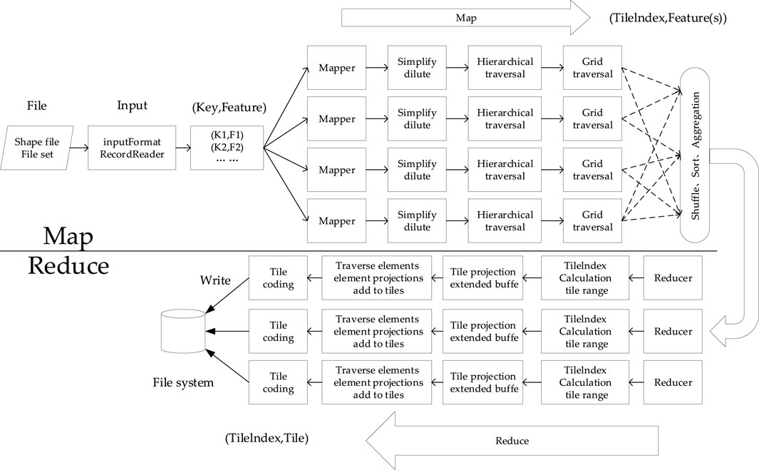
FIGURE 5. Map vector tile parallel construction process.
The intermediate results of the Map phase are finally obtained through aggregation [TileIndex, Feature(s)] as input parameters of the customized reduce function. In the reduce stage, the four corner coordinates of the tiles are calculated backward according to TileIndex and empty tiles are generated. Then, the projection transformation and other processing of the tiles are carried out to ensure that the tiles and the element geometry are in the same spatial reference system. The buffer of the tile is extended to ensure that the tile can be seamlessly joined when rendering. The size of the extended buffer depends on the actual situation. Tiles are organized in a tile–layer-feature hierarchical structure. One tile can contain multiple layers, and multiple feature elements can be added to one layer. The elements are added to the tiles for cutting and coding. Multiple reduce subtasks are encoded in parallel to obtain tile data and output the file to the storage system as a binary byte stream. Tiles are stored in a level-X-Y directory tree structure. The file is named Y.pdf.
The patchiness of the cultivated land map refers to the compactness and continuity of cultivated land distribution, which is of great significance for agricultural production, ecological environment protection, land resource utilization, and other aspects (Muchova et al., 2017; Wang et al., 2017). The cultivated land with good connectivity is conducive to agricultural mechanization, reducing agricultural production costs and improving labor productivity and crop yield. At the same time, the cultivated land with good connectivity can reduce the fragmentation of land use, which is conducive to the stability of the ecosystem and the protection of biodiversity (Gomes et al., 2019). This paper analyzes the spatial connectivity of GIS patch data based on map vector slices to improve the computational efficiency.
There are two parts in the process of constructing the pattern patch network. First, a buffer is generated for each pattern patch. Second, the intersection of each pattern spot and other pattern spots is calculated. As shown in Figure 6, the first part is relatively simple; it can directly generate the basic buffer, without the need to merge the buffer, this section mainly from the intersection between the map spot expansions. In GIS spatial analysis, superposition analysis is the basic method of comparison, which includes superposition, intersection, and symmetric difference among points, lines, and surfaces. This paper mainly involves the operation to determine whether two graph spots intersect in the superposition analysis. Based on the grid computing unit and grid index established in the previous section, a spatial analysis algorithm that can be processed by MapReduce is further designed to carry out the intersection operation of graph spots after reading local spatial indexes.
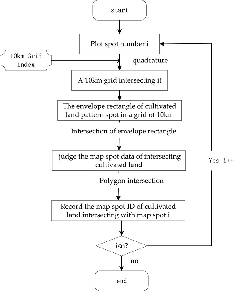
FIGURE 6. Flowchart of the polygon intersection.
The aforementioned graph spot intersection data are the connection between each graph spot and other graph spots. Taking the center point of a graph spot as a node, these intersection relations are connected into lines, that is, a graph spot interconnection network is formed.
Before calculating the linkage index of graph spots, it is necessary to first determine the basic information on other graph spots within the maximum number of connections with each graph spot and use the Dijkstra algorithm to calculate the minimum number of links between them, and then determine the link weight between them according to the quality of the two graph spots. On the basis of the minimum number of links and the link matrix, the local joint degree of each pattern spot can be calculated using the formula. Finally, the local connectivity of each spot is summarized, and the global connectivity of each grid is calculated. The specific process is shown in Figure 7.
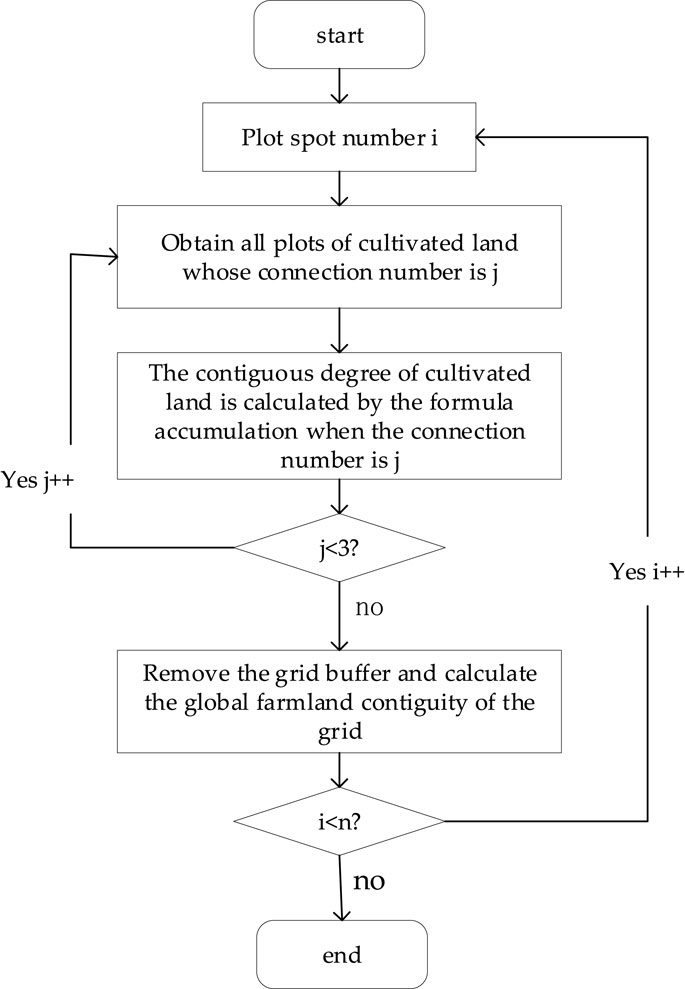
FIGURE 7. Calculation process of the spatial connectivity index.
In this paper, the maximum number of connections is 3. Based on the aforementioned calculation process of the degree of the graph spot alignment, the parallelization of the degree of the graph spot alignment is realized using the MapReduce parallelization algorithm. In this paper, the MapReduce parallel algorithm is implemented through a Job. The parallel processing steps are given as follows:
Input: Patch contiguous network, stored in junction class.
Output: Local contiguity of each pattern spot.
Steps:
1) Before the operation of the Map phase, read all the graph patch connected network data in the computing grid into the memory, and store all junction data in it into HashMap to ensure that the data can be read at any time.
2) In the Map stage, complete the joint degree calculation of a single map spot. Perform the following operations: in the Map operation, key is the id of each node and value is the basic attribute information and connection information on the spot stored by each node. Perform the following operations for the entire data block:
2.1) Obtain information about other nodes connected to this node through HashMap.
2.2) Calculate the connectedness value of 1, obtain the information on nodes with two connectedness through recursion, and add the connectedness value, until all patches within the maximum number of connectedness are calculated.
2.3) Shuffle the calculated result with the grid ID as the key value.
3) In the reduce phase, the output result of the Map function is analyzed according to the key–value pair, where the key is the ID of the grid and the value is the basic information on each map spot. The reduce function is used to sum up the pattern spot results of each grid, and the formula is used to calculate the global slice value of each grid. Finally, the value of the global connectedness and the value of the connectedness of each spot are stored according to the grid.
Three services were used to form a cluster in the experiment environment. The operating system environment configured for each machine was Ubuntu 18.04, the CPU was 2 Intel E5-2620v4 CPUs (8 cores and 16 threads), and the memory was 32 GB. Each machine is configured with Java Development Kit (JDK)1.8 and Hadoop 3.1.3. There are four groups of experimental data, namely, global administrative data, China water distribution data, global lake data, and global building data. Both of them are planar data, and the data size is shown in Table 2. The source data is one shapefile file. The data are pre-divided into nine shapefiles to ensure that each node can participate in the calculation process in the case of multiple nodes in parallel.
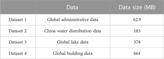
TABLE 2. Test datasets.
The first set of experiments tested the feasibility of the algorithm in a multi-node environment and constructed vector tiles of the four test data at levels 0–11. Each level constructed and recorded its time. In the second experiment, four groups of experimental data were used to test the construction time of different number of nodes, build levels from 0 to 10, and record the total time. All the aforementioned experiments were repeated eight times, and the average time was taken as the result. The third experiment is to compare with the traditional ArcGIS model, reflecting the progressiveness of the method in this paper. Experiment 4 conducted tests on different nodes for spatial connectivity calculation in the cluster, and finally, combined with national data, and produced and analyzed a thematic map of farmland spatial connectivity.
The test results of vector tile construction at each level are shown in Figure 8. From the figure, it can be seen that as the tile level increases, the number of tiles increases and the construction time also increases. At lower levels, such as 0–1, the time consumption is almost the same for different datasets, which is because creating Map and Reduce tasks consumes a larger proportion of time, while a small amount of tiles in parallel have almost the same computational time. When the number of tiles increases, the proportion of time spent on tile generation is greater, so the total time consumption increases as the number of tiles increases. If the original data are a single shapefile file, the data need to be divided into multiple blocks in order to achieve the parallelism of the Map task in the multi-node calculation.
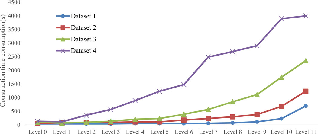
FIGURE 8. Construction time consumption of vector tiles at different levels.
From Figure 8, we can also see that there are significant differences between different datasets. Overall, the larger the data volume, the longer the time it takes.
The second group of experiments used the aforementioned four types of data to construct vector tiles at levels 0–10 with different numbers of nodes. The experiment was also repeated eight times, and the total consumption time was recorded before taking the average. The test results are shown in Figure 9. From the perspective of time comparison, horizontally expanding multi-node parallelization can greatly improve the efficiency of vector tile parallel construction, with single node and dual node comparisons being the most obvious. In a single node, multiple Map and Reduce tasks are applied for, but they are still executed serially, and the Reduce task is only executed after the Map task ends. In multiple nodes, multiple Map tasks can be executed simultaneously, and the execution time of each Map task varies. Therefore, the node that completes the Map task first can start the Reduce task in advance, thereby improving efficiency.

FIGURE 9. Construction time consumption of vector tiles with different number of nodes.
In summary, when constructing a small amount of tiles with a small amount of data, using multiple nodes to construct vector tiles reduces efficiency. Because in a multi-node environment, most of the time is spent on creating tasks and processes, and scheduling resources; it is advisable to consider using a single machine to build vector tiles; under the condition of constructing large-scale vector tiles, the ability of parallel computing can be fully utilized.
As can be seen from Figure 10, the calculation efficiency of the polygon alignment degree proposed in this paper is higher than that of ArcGIS engine in a single-machine environment, with a difference of more than five times. As can be seen from Figure 11, the clustering mode can further improve the computing efficiency.

FIGURE 10. Comparison of the calculation efficiency of spatial connectivity.
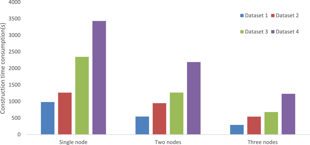
FIGURE 11. Computing efficiency comparison of spatial connectivity in the cluster environment.
The national arable land calculation results are shown in Figure 12. This article divides the cultivated land results into high contiguous areas, medium contiguous areas, and low contiguous areas using the equal spacing method, represented by three colors, namely, green, blue, and red, respectively (the two square blanks in Northeast Liaoning id due to data calculation errors and legends cannot be added due to the national data being drawn by the spatial Hadoop cluster). From the figure, it can be seen that the cultivated land in Northeast and North China has a higher degree of connectivity, while the cultivated land in Southeast and Southwest China has a lower degree of connectivity, which is consistent with the actual situation in China. The Northeast and North China regions are located in plains, with flat terrain, large plot areas, and regular shapes, with relatively concentrated and contiguous cultivated land. However, the Southeast and Southwest China regions are mostly hilly and mountainous areas, with scattered and fragmented plot distribution, irregular shape, and poor concentrated and contiguous cultivated land.
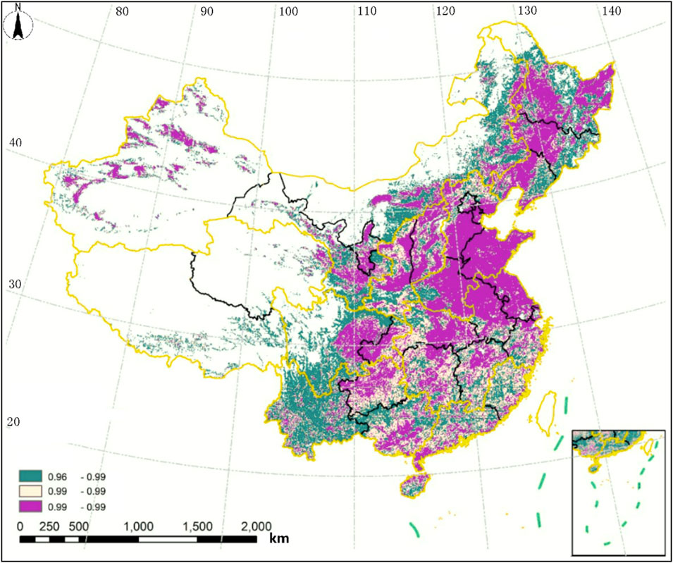
FIGURE 12. Schematic diagram of spatial connectivity analysis of national arable land.
For the construction of vector tiles for large-scale vector data, efficiency and quality are two highly concerned aspects. The performance of a single machine construction can no longer meet the needs of data production, while parallelization schemes can greatly improve the efficiency of construction; the quality of vector tiles requires consideration of data simplification and synthesis issues during the construction process. Therefore, this article proposes a vector tile parallel construction algorithm based on the MapReduce parallel programming model. Both groups of experiments prove the feasibility of the proposed algorithm, which can significantly improve the efficiency of vector tile construction in the multi-node cluster environment.
This paper summarizes the key technologies of vector tile construction and introduces the algorithm flow of vector tile parallel construction based on the MapReduce parallel programming model in detail. The experiment verifies the feasibility of the static cache vector tile scheme of this algorithm and significantly improves the construction efficiency of the vector tile. At the same time, the algorithm of spatial connectivity analysis of the planar graph is applied. However, there are still some shortcomings, for example, simplification and thinning strategies need to be considered from multiple perspectives. Only using the Douglas–Peucker algorithm cannot meet the simplification requirements of vector data, and the algorithm still has room for optimization.
Publicly available datasets were analyzed in this study. These data can be found online at: https://www.openstreetmap.org/.
Conceptualization, formal analysis, investigation, resources, data curation, writing—original draft preparation, writing—review and editing, visualization, supervision, and project administration: SM; validation: SM and SZ; and funding acquisition: SZ. All authors contributed to the article and approved the submitted version.
The authors are grateful for the comments and contributions of the reviewers and the members of the editorial team.
The authors declare that the research was conducted in the absence of any commercial or financial relationships that could be construed as a potential conflict of interest.
All claims expressed in this article are solely those of the authors and do not necessarily represent those of their affiliated organizations, or those of the publisher, the editors, and the reviewers. Any product that may be evaluated in this article, or claim that may be made by its manufacturer, is not guaranteed or endorsed by the publisher.
Alarabi, L., Mokbel, M. F., and Musleh, M. (2018). ST-hadoop: a MapReduce framework for spatio-temporal data. GeoInformatica 22, 785–813. doi:10.1007/s10707-018-0325-6
Eldawy, A., and Mokbel, M. F. (2015). “SpatialHadoop: A MapReduce framework for spatial data,” in Proceedings of the 2015 IEEE 31st International Conference on Data Engineering, Seoul, Korea (South), 13-17 April 2015, 1352–1363.
Gomes, E., Banos, A., Abrantes, P., Rocha, J., Kristensen, S. B. P., and Busck, A. (2019). Agricultural land fragmentation analysis in a peri-urban context: from the past into the future. Ecol. Indic. 97, 380–388. doi:10.1016/j.ecolind.2018.10.025
Guo, N., Xiong, W., Wu, Q., and Jing, N. (2016). An efficient tile-pyramids building method for fast visualization of massive geospatial raster datasets. Adv. Electr. Comput. Eng. 16, 3–8. doi:10.4316/aece.2016.04001
Huang, L., Meijers, M., uba, R., and Van Oosterom, P. (2016). Engineering web maps with gradual content zoom based on streaming vector data. ISPRS J. Photogrammetry Remote Sens. 114, 274–293. doi:10.1016/j.isprsjprs.2015.11.011
Jia, Y., Wu, J., and Sarwat, M. (2015). “GeoSpark: A cluster computing framework for processing large-scale spatial data,” in Proceedings of the the 23rd SIGSPATIAL International Conference, Washington, Seattle, November 3 - 6, 2015.
Li, Q., and Li, D. (2014). Big data GIS. Wuhan Daxue Xuebao (Xinxi Kexue Ban)/Geomatics Inf. Sci. Wuhan Univ. 39, 641–666. doi:10.13203/j.whugis20140150
Li, S., Dragicevic, S., Castro, F. A., Sester, M., Winter, S., Coltekin, A., et al. (2016). Geospatial big data handling theory and methods: A review and research challenges. ISPRS J. Photogrammetry Remote Sens. 115, 119–133. doi:10.1016/j.isprsjprs.2015.10.012
Liu, P., Xu, X., and Yang, M. (2022). An improved schema for vector tile map considering symbol integrity. Wuhan Daxue Xuebao (Xinxi Kexue Ban)/Geomatics Inf. Sci. Wuhan Univ. 47, 455–462. doi:10.13203/j.whugis20200033
Muchova, Z., Leitmanova, M., and Michal, P. (2017). “PRE and post land consolidation land fragmentation assessment,” in Proceedings of the 17th International Multidisciplinary Scientific GeoConference, SGEM 2017, Albena, Bulgaria, June 29, 2017 - July 5, 2017, 461–468.
Ramos, J. A. S., Esperanca, C., and Clua, E. W. G. (2009). A progressive vector map browser for the web. J. Braz. Comput. Soc. 15, 35–48. doi:10.1007/bf03194500
Wan, L., Huang, Z., and Peng, X. (2016). An effective NoSQL-based vector map tile management approach. ISPRS Int. J. Geo-Information 5, 215. doi:10.3390/ijgi5110215
Wang, J., Liem, P. D., Linh, V. N., and Ha, T. T. V. (2017). Impacts of land fragmentation on the development of agriculture and agricultural mechanization in Vietnam. Int. Agric. Eng. J. 26, 156–164.
Wang, W., Yao, X., and Chen, J. (2022). A map tile data access model based on the jump consistent hash algorithm. ISPRS Int. J. Geo-Information 11, 608. doi:10.3390/ijgi11120608
Yan, X., Ai, T., Zhang, X., and Yang, W. (2018). A vector pyramid model to support continuous multi-scale representation of spatial data. Wuhan Daxue Xuebao (Xinxi Kexue Ban)/Geomatics Inf. Sci. Wuhan Univ. 43, 502–508. doi:10.13203/j.whugis20150723
Yang, C., Xu, Y., and Nebert, D. (2013). Redefining the possibility of digital Earth and geosciences with spatial cloud computing. Int. J. Digital Earth 6, 297–312. doi:10.1080/17538947.2013.769783
Yang, C., Yu, M., Hu, F., Jiang, Y., and Li, Y. (2017). Utilizing Cloud Computing to address big geospatial data challenges. Comput. Environ. Urban Syst. 61, 120–128. doi:10.1016/j.compenvurbsys.2016.10.010
Yao, X., and Li, G. (2018). Big spatial vector data management: a review. Big Earth Data 2, 108–129. doi:10.1080/20964471.2018.1432115
Yao, X., Mokbel, M., Ye, S., Li, G., Alarabi, L., Eldawy, A., et al. (2018a). LandQv2: A MapReduce-based system for processing arable land quality big data. ISPRS Int. J. Geo-Information 7, 271. doi:10.3390/ijgi7070271
Yao, X., Yang, J., Li, L., Ye, S., Yun, W., and Zhu, D. (2018b). Parallel algorithm for partitioning massive spatial vector data in cloud environment. Wuhan Daxue Xuebao (Xinxi Kexue Ban)/Geomatics Inf. Sci. Wuhan Univ. 43, 1092–1097. doi:10.13203/j.whugis20160271
Yao, X., Yu, G., Li, G., Yan, S., Zhao, L., and Zhu, D. (2023). HexTile: A hexagonal DGGS-based map tile algorithm for visualizing big remote sensing data in spark. ISPRS Int. J. Geo-Information 12, 89. doi:10.3390/ijgi12030089
Zhou, M., Chen, J., and Gong, J. (2016). A virtual globe-based vector data model: quaternary quadrangle vector tile model. Int. J. Digital Earth 9, 230–251. doi:10.1080/17538947.2015.1016558
Keywords: map vector tile, visualization, spatial connectivity analysis, arable land, Hadoop
Citation: Ma S and Zhang S (2023) Map vector tile construction for arable land spatial connectivity analysis based on the Hadoop cloud platform. Front. Earth Sci. 11:1234732. doi: 10.3389/feart.2023.1234732
Received: 05 June 2023; Accepted: 16 August 2023;
Published: 29 August 2023.
Edited by:
Houda Harkat, Instituto de Desenvolvimento de Novas Tecnologias (UNINOVA), PortugalReviewed by:
Liangcun Jiang, Wuhan University of Technology, ChinaCopyright © 2023 Ma and Zhang. This is an open-access article distributed under the terms of the Creative Commons Attribution License (CC BY). The use, distribution or reproduction in other forums is permitted, provided the original author(s) and the copyright owner(s) are credited and that the original publication in this journal is cited, in accordance with accepted academic practice. No use, distribution or reproduction is permitted which does not comply with these terms.
*Correspondence: Shengting Ma, MjIyMDIxMTAyOUBkbG11LmVkdS5jbg==
Disclaimer: All claims expressed in this article are solely those of the authors and do not necessarily represent those of their affiliated organizations, or those of the publisher, the editors and the reviewers. Any product that may be evaluated in this article or claim that may be made by its manufacturer is not guaranteed or endorsed by the publisher.
Research integrity at Frontiers
Learn more about the work of our research integrity team to safeguard the quality of each article we publish.