Effect of temperature on carbon accumulation in northern lake systems over the past 21,000 years

Introduction: Rising industrial emissions of carbon dioxide and methane highlight the important role of carbon sinks and sources in fast-changing northern landscapes. Northern lake systems play a key role in regulating organic carbon input by accumulating carbon in their sediment. Here we look at the lake history of 28 lakes (between 50°N and 80°N) over the past 21,000 years to explore the relationship between carbon accumulation in lakes and temperature changes.

Method: For this study, we calculated organic carbon accumulation rates (OCAR) using measured and newly generated organic carbon and dry bulk density data. To estimate new data, we used and evaluated seven different regression techniques in addition to a log-linear model as our base model. We also used combined age-depth modeling to derive sedimentation rates and the TraCE-21ka climate reanalysis dataset to understand temperature development since the Last Glacial Maximum. We determined correlation between temperature and OCAR by using four different correlation coefficients.

Results: In our data collection, we found a slightly positive association between OCAR and temperature. OCAR values peaked during warm periods Bølling Allerød (38.07 g·m⁻²·yr⁻¹) and the Early Holocene (40.68 g·m⁻²·yr⁻¹), while lowest values occurred during the cold phases of Last Glacial Maximum (9.47 g·m⁻²·yr⁻¹) and Last Deglaciation (10.53 g·m⁻²·yr⁻¹). However, high temperatures did not directly lead to high OCAR values.

Discussion: We assume that rapid warming events lead to high carbon accumulation in lakes, but as warming progresses, this effect appears to change as increased microbial activity triggers greater outgassing. Despite the complexity of environmental forcing mechanisms affecting individual lake systems, our study showed statistical significance between measured OCAR and modelled paleotemperature for 11 out of 28 lakes. We concluded that air temperature alone appears to drive the carbon accumulation in lakes. We expected that other factors (catchment vegetation, permafrost, and lake characteristics) would influence accumulation rates, but could not discover a conclusive factor that had a statistical significant impact. More data available on long-term records from northern lake systems could lead to more confidence and accuracy on the matter.

1 Introduction

Northern lake systems (50°N–80°N) have been subject to an increase in mean annual surface air temperature up to 2.7°C over the last few decades (Box et al., 2019; Meredith et al., 2019; Ballinger et al., 2020). Temperature is one of the key control variable for the mineralization and burial of carbon in lakes, regardless of the origin of carbon (i.e., autochthonous or allochthonous) (Gudasz et al., 2010; Gudasz et al., 2015). Not only is an increase in temperature associated with higher carbon mineralization and burial, but also favors higher turnover of carbon through more in-lake primary production by macrophytes/aquatic plants (Li et al., 2017; Velthuis et al., 2018) and algae (Biskaborn et al., 2022). As a consequence, lake systems can shift from being a net carbon sink to net carbon source and vice versa (Sobek et al., 2014; Heathcote et al., 2015; Denfeld et al., 2018).

Dean and Gorham (1998) estimated that lakes on a global scale accumulate in their sediment about 42 TgC (teragrams of carbon, i.e., one million metric tons of carbon) per year. Based on a new modeling approach, Anderson et al. (2020) approximated that accumulation rates have almost tripled over the past 100 years by about 72 TgC from 0.05 PgC to 0.12 PgC per year. In this model, the authors estimated that lakes in boreal biome contribute the highest (24%) to the global carbon burial rate, while tundra lakes are the lowest at only 2% due to their low carbon burial rate (Anderson et al., 2020). Despite potentially lower carbon burial rates in northern lakes due to current lower temperatures (Gudasz et al., 2010), Sobek et al. (2014) found that Arctic lakes show similar burial efficiencies as other lakes at lower latitudes. In addition, climate change-induced shifts in vegetation (Cramer et al., 2001; Pearson et al., 2013), lake aquatic biomass production (Biskaborn et al., 2023), and increased carbon release from permafrost thawing (Meredith et al., 2019; Schuur et al., 2022) may raise carbon burial rates in Arctic lakes due to the growing availability of carbon within the lakes (Anderson et al., 2020).

Comprehending the complex burial process requires a thorough understanding of how the carbon cycle in a lake responds to temperature fluctuations. Temperature plays a crucial role in shaping the interactions between dissolved organic carbon (DOC) and dissolved inorganic carbon (DIC) in lake ecosystems (Gudasz et al., 2010). DIC comprises carbon in the form of inorganic carbon species, primarily bicarbonate (HCO₃⁻), carbonate (CO₃⁻²), and dissolved carbon dioxide (CO₂), while DOC refers to the fraction of organic carbon compounds dissolved in water. Higher temperatures can enhance microbial activity, leading to increased breakdown of organic matter and subsequent release of DOC into the lake water (Middelboe and Lundsgaard, 2003; Adams et al., 2010). This process elevates the concentration of DOC in the lake, which influences organic carbon burial rates in lake sediments. Additionally, raised temperatures promote primary production by aquatic plants and algae, which enhances photosynthesis and the uptake of DIC from the water column (Hein, 1997; Hammer et al., 2019). As a result, this process can either increase the outgassing of CO₂ from the lake or promote more carbonate precipitation of carbonated minerals within the lake.

In-lake bioproductivity and carbon accumulation also depend on catchment vegetation and the availability of allochthonous carbon (Roiha et al., 2016). During the Last Glacial Maximum, sparse vegetation and a reduced flux of allochthonous carbon to the lakes prevailed the Arctic due to the severe climatic conditions (Melles et al., 2012). In most areas the lack of nutrients in the underlying permafrost soil prevented further advances of boreal forests (Sundqvist et al., 2014). However, as the climate warmed and glaciers retreated, vegetation types shifted from tundra to boreal forest, which substantially increased the availability of organic carbon (Lozhkin et al., 2007; Lozhkin et al., 2018; Biskaborn et al., 2016; Diekmann et al., 2017).

Nutrient fertilization and atmospheric deposition played a crucial role in the Holocene in enhancing the productivity of the Arctic vegetation (Galloway et al., 2004; Choudhary et al., 2016). A prolonged growing season due to a warmer climate and shorter ice coverage further contributes to an upsurge in carbon turnover within lakes (Walther et al., 2002; Vuglinsky and Valatin, 2018; Sharma et al., 2019; Sharma et al., 2020). However, eutrophication and browning can in turn negate these effects, leading to stable water stratification with anoxic conditions at the bottom of the lake (Bartosiewicz et al., 2019).

In addition to in-lake primary productivity, other factors can affect the overall carbon balance within a lake, such as sediment resuspension/re-mineralization (Guillemette et al., 2017; Klump et al., 2020), or lake characteristics (e.g., morphology, catchment characteristics, or geographical location) (Ferland et al., 2014; Clow et al., 2015; Denfeld et al., 2018; Zwart et al., 2019). Nevertheless, changes in land use and changing precipitation patterns will in turn affect the distribution and storage of carbon in the Arctic in the future (Tchebakova et al., 2009; Bartsch et al., 2016; Windirsch et al., 2022).

While studies have focused on the carbon balance of lakes in the Holocene (e.g., Anderson et al., 2009; Sobek et al., 2014; Heathcote et al., 2015), investigations into past carbon accumulation rates back to the Late Pleistocene are lacking. Since the burial of organic carbon can react sensitively to temperature changes (Gudasz et al., 2010; Gudasz et al., 2015), a longer observation period with larger temperature differences can reveal new perspectives. To test whether temperature is the key driver in northern high-latitude lakes, we need to consider other influencing factors in our analysis, such as catchment vegetation, underlying permafrost, and lake-specific properties.

The main objective of this paper is to investigate the relationship between temperature and carbon in northern lakes over the past 21,000 years. We estimate the amount of carbon accumulated in 28 lakes since the Late Pleistocene using a combination of measured and newly generated organic carbon and dry bulk density data. To generate new data, we test seven different regression techniques as prediction models and evaluate them against common assessment metrics. We then correlate the obtained accumulation rates with temperature from re-analysis data (TraCE-21ka climate reanalysis dataset) to understand the relationship between these rates and changing temperature. Given the large time span covered by the datasets and the geographic spread of the sediment cores, we further create relationships to permafrost, vegetation, and lake-specific attributes.

2 Materials and methods

To determine the amount of carbon that accumulated over the past 21,000 years, we need to calculate the “organic carbon accumulation rate” (OCAR, in g·m⁻²·yr⁻¹) using the following equation (Eq. 1):

$OCAR=\left(DBD\times \left(\frac{TOC}{100}\right)\right)\times SR(1)$

where DBD is dry bulk density (in g·cm⁻³), TOC is the total organic carbon content (in weight-%), and SR is the age-depth-model-derived sedimentation rate (in cm·yr^-1). We divided the resulting unit (g·cm⁻²·yr⁻¹) by 0.0001 to get the desired OCAR unit (g·m⁻²·yr⁻¹).

To acquire the necessary data for this project, we conducted a comprehensive data collection process that focused on TOC and DBD measurements. In total, we collected 28 datasets from high latitude lake systems (50°N–80°N—Figure 1) containing TOC, which we standardized following the procedure introduced by Pfalz et al. (2021). In addition to DBD and TOC, our data collection focused on two additional data series: 1) sediment water content (WC) data, and 2) grain size measurements divided into the three subgroups of sand, silt, and clay (in weight-%).

FIGURE 1

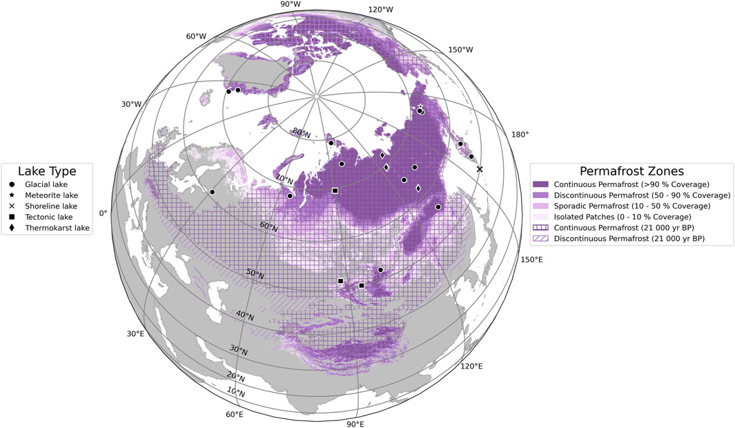
FIGURE 1. Spatial distribution of sediment cores from northern lakes (50°N–90°N) used in this study labeled by their lake type (black symbols, n = 28). Underlying permafrost zones for the present time (solid colored areas) are from Obu et al. (2019), while permafrost distribution of the last 21,000 years (shaded areas) originates from Lindgren et al. (2016). We adapted the color scheme for permafrost zones (four different shades of purple) from Obu et al. (2019) to be consistent with the original publication.

Given the variable data availability of sediment cores with DBD, we divided the sediment cores into two subgroups: “Complete datasets” and “Augmented datasets” (Table 1). “Complete datasets” consist of subsets of sediment cores that contain (C1) DBD, TOC, sand, silt, and WC data, (C2) Wet bulk density, TOC, and WC data, and (C3) both DBD and TOC. On the other hand, “Augmented datasets” refer to datasets that were lacking DBD information but had (A1) grain size and partially WC data available or (A2) neither grain size nor WC data available.

TABLE 1

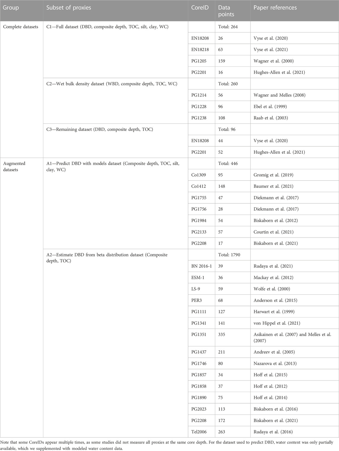
TABLE 1. Summary table containing individual datasets used for this study.

While both C1 and C3 datasets were directly usable for OCAR calculation, in three instances of our data collection (subset C2—“Wet bulk density dataset”—Table 1), we collected values for wet bulk density instead of dry bulk density. Because these datasets also provided data on the water content, we were able to calculate dry bulk density with the following equation (Eq. 2):

$DBD=\left(1-\left(\frac{WC}{100}\right)\right)\times WBD(2)$

with DBD being dry bulk density (in g·cm⁻³), WC being the water content (in weight-%), and WBD being the wet bulk density (in g·cm⁻³).

As both “augmented datasets” A1 and A2 were lacking DBD measurements, we considered predicting DBD from existing data. A large number of empirically derived pedotransfer functions and techniques for predicting bulk density exist in the literature (e.g., Hollis et al., 2012; Martín et al., 2017; Lu et al., 2021; Palladino et al., 2022; Qin et al., 2022). The majority of these prediction techniques use variations of linear models to predict bulk density. To enable comparison with the existing literature, we decided to use a log-linear model as our base model, which we built in Python using “scikit-learn” and its “LinearRegression” function (Pedregosa et al., 2012).

In contrast to other pedotransfer functions, we included both the depth of a given sample within the sediment core (in cm) and its water content, which gave us the following equation (Eq. 3):

$\ln \left(DBD\right)=\alpha +{\beta }_1\times \left(CDepth\right)+{\beta }_2\times \left(TOC\right)(3)$

$+{\beta }_3\times \left(Silt\right)+{\beta }_4\times \left(Clay\right)+{\beta }_5\times \left(WC\right)$

where DBD is dry bulk density (in g·cm⁻³), CDepth is the composite depth below sediment surface (as mid-point cm), TOC is total organic carbon content (in mg·g⁻¹), Silt and Clay are the silt and clay content from grain size measurements (in weight ratios), WC is the water content (in weight-%), α is the intercept, and β₁ to β₅ are the individual coefficients. We obtained the unit “mg·g⁻¹” for the TOC measurements by multiplying weight percent by factor 10, and unit “weight ratios” for clay and silt data by dividing the weight percent by factor 100.

Considering the significant impact of sediment water content on sediment compaction, we recognized its importance in predicting DBD. However, 11 sediment core datasets (39% of the collected datasets) lacked water content data. To address this limitation and to test whether other regression methods can outperform linear models, we decided to predict WC alongside DBD in several multiple output regression methods in addition to the linear model. We opted for non-linear machine learning techniques to allow for a better comparison with the (non-linear) log-linear model. This includes the following regression methods from the “scikit-learn” and “xgboost” package in Python (Pedregosa et al., 2012; Chen and Guestrin, 2016):

• Random Forest Regression

• Extreme Gradient Boosting (XGBoost)

• Gradient Boosting

• K-nearest Neighbor

• Support Vector Regression

• AdaBoost Regression.

For training and evaluation purposes, we split the “Full dataset” C1 (Table 1) into a training (80%) and test set (20%), but also used fivefold cross-validation to alleviate potential biases in the splitting process. We scored the individual models by using the following metrics: mean absolute error (MAE), relative absolute error (RAE), mean squared error (MSE), root mean squared error (RMSE), root relative squared error (RRSE), and R² score. The Supplementary Material contains the equations used for these metrics. We further checked if hyperparameter tuning would improve our results by adding an additional pipeline with the “GridSearchCV” and “RandomizedSearchCV” optimization algorithms from the “scikit-learn” package (Pedregosa et al., 2012).

For subset A1, we used the log-linear model and the regression methods to predict DBD and, where necessary, WC. However, for subset A2 (“Estimate DBD from beta distribution dataset”—Table 1), we only had TOC measurements for 15 sediment cores available for bulk density prediction. We therefore used existing grain size data from eleven sediment cores in the data collection (710 data points) to generate beta distributions for clay and silt. These beta distributions rely on the two parameters α_beta and β_beta, which we individually calculated using the following two equations (Eqs 4, 5):

${\alpha }_{beta}=\left(\frac{1-\mu }{{\sigma }^2}-\frac{1}{\mu }\right)\times {\mu }^2(4)$

${\beta }_{beta}={\alpha }_{beta}\times \left(\frac{1}{\mu }-1\right)(5)$

with µ and σ² being the mean and the variance of the existing clay or silt data, respectively. After obtaining α_beta and β_beta values for both clay and silt content, we drew 10,000 silt and clay values for each TOC measurement from the newly constructed beta distributions using “random sampling” of the Python package “numpy” (Harris et al., 2020). To reduce overall computing time, we performed random sampling and subsequent prediction of dry bulk density (Eq. 3) in parallel using the “Dask” back-end (Dask Development Team, 2016) and the “joblib” Python package (Joblib Development Team, 2020).

However, we constrained the possible values for clay and silt in two ways before using them in our models to predict dry bulk density ranges. Given that grain size data is compositional data, i.e., the sum of its components should add up to 1% or 100% (Greenacre, 2021), we first removed sums of clay and silt weight ratios that were greater than one. Since grain size data consists of a third component, which is the grain size range for sand, we also considered a lower bound for the sums to account for sand occurrence in the sediment cores. From the given data, we estimated that a maximum of 20% sand in the sediment column would be possible for our data collection. Therefore, we also removed sums of clay and silt weight ratios that were smaller than 0.8.

In any case, working with modeled values can introduce potential errors that could affect the interpretation of results. The quality and accuracy of the input data play a crucial role in determining the model’s performance and output (Rebba et al., 2006; Huang and Laffan, 2009). Errors during data collection or sample measurement can propagate into the model outputs. We mitigated the risk by relying on original raw data as much as possible and used a database to ensure the values fell within physically plausible ranges (Pfalz et al., 2021). While both Eqs 1, 3 represent simplifications of complex systems, and overly simplistic models can overlook important processes that lead to incorrect results (Andersson et al., 1999; Mathews and Vial, 2017). However, we struck a balance between simplification and computational feasibility, using only publicly available data and ensuring the reproducibility of our results.

We used the LANDO age-depth modeling result from Pfalz et al. (2022) to derive sedimentation rates (SR) for each sediment core. LANDO links five age-depth modeling systems (Bacon, Bchron, clam, hamstr, Undatable) in one multi-language Jupyter Notebook (Haslett and Parnell, 2008; Parnell et al., 2008; Blaauw, 2010; Blaauw and Christen, 2011; Kluyver et al., 2016; Peng et al., 2018; Lougheed and Obrochta, 2019; Dolman, 2022). For all sediment cores, we combined the results from the five modeling systems with standard settings into an ensemble model with two-sigma uncertainty [as described in Pfalz et al. (2022)]. We propagated these sedimentation rate uncertainties into the OCAR calculations (Eq. 1) to obtain OCAR uncertainty ranges.

To understand the temperature development since the Last Glacial Maximum (Clark et al., 2009), we used the TraCE-21ka climate reanalysis dataset (He, 2011), which we will refer to simply as TraCE dataset hereinafter. We divided the timespan covered by the TraCE dataset into the following periods (Walker et al., 2019; Head et al., 2021; Kuang et al., 2021):

• Last Glacial Maximum—22,000 to 18,000 years BP (years before present, i.e., before 1950 CE)

• Last Deglaciation—18,000 to 14,300 years BP

• Bølling Allerød—14,300 to 12,700 years BP

• Younger Dryas—12,700 to 11,700 years BP

• Early Holocene—11,700–8,200 years BP

• Mid-Holocene—8,200 to 4,200 years BP

• Late Holocene—4,200 years BP to present.

For each core location, we extracted the surface air temperature at reference height (TREFHT) from the nearest grid cell of the TraCE dataset [grid cell resolution: 2.5° × 2.5° (He, 2011; Brown et al., 2020)]. We then converted the temperature from Kelvin (K) to Celsius (°C) by subtracting 273.15 K from each value and then averaging values for the summer months June-July-August (JJA). Following the procedure introduced by Kaufman et al. (2020a), we converted OCAR values to z-score. The z-score measures how many standard deviations each point is away from the mean, and thus normalizes the data. To comprehend how vegetation affects carbon accumulation, we used the vegetation reconstruction by Dallmeyer et al. (2022) (depicted in Figure 2), which incorporates the TraCE dataset into its remodeling.

FIGURE 2

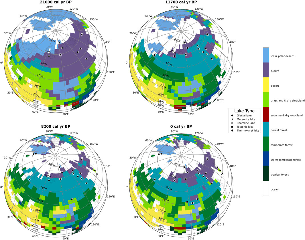
FIGURE 2. Biome distribution based on Dallmeyer et al. (2022) vegetation reconstruction for the past 21,000 years represented in four snapshots (21,000, 11,700, 8,200, and 0 calibrated years Before Present, i.e., before 1950 Common Era). We include sediment cores with their respective lake type in the snapshot if there is TOC data available for them (black symbols).

To determine the correlation between temperature and OCAR, we first had to check for normality of the two variables. For this reason, we visually inspected the data by plotting quantile-quantile plots (Q-Q plots) using the package “statsmodels” (Seabold and Perktold, 2010). We then used both the Shapiro-Wilk as well as the D’Agostino and Pearson’s test from the Python package “scikit-learn” (Pedregosa et al., 2012) for our statistical tests. As both temperature and OCAR did not display normality, we used Spearman’s and Chatterjee’s rank correlation coefficient to check for the correlation between the two variables. In contrast to Chatterjee’s coefficient, Spearman’s coefficient is a well-established, robust correlation metric often used for variables from non-normal distributions (Sadeghi, 2022). However, the Chatterjee’s coefficient showed promising results for testing the non-linear functional correlation between two variables (Chatterjee, 2021; Sadeghi, 2022). In addition to the Spearman and Chatterjee correlation coefficient, we checked the Pearson and Kendall-Tau correlation coefficient on both the untransformed and z-transformed variables. The methods for the more common correlation coefficients came from the Python package “scipy” (Virtanen et al., 2020), while to calculate the Chatterjee coefficient we used the script provided by Chatterjee (2021).

3 Results

While our data collection yielded 620 data points (Table 1—Complete datasets) containing DBD and TOC which were directly usable for OCAR calculation (Eq. 1), the majority of data points from the augmented datasets (n = 2,236, Table 1—Augmented datasets) required further calculations. In preparation for both A1 and A2, we fitted the log-linear model with training dataset of our subset C1 (Table 1—“Full dataset”) to obtain the following equation to predict dry bulk density using a linear regression:

$\ln \left(DBD\right)=1.3337+0.0001\times \left(CDepth\right)-0.0016\times \left(TOC\right)$

$-0.3986\times \left(Silt\right)+0.353\times \left(Clay\right)-0.0267\times \left(WC\right)(6)$

where DBD is dry bulk density (in g·cm⁻³), CDepth is the composite depth below sediment surface (as mid-point cm), TOC is total organic carbon content (in mg·g⁻¹), Silt and Clay are the silt and clay content from grain size measurements (in weight ratios), WC is the water content (in weight-%).

Since we wanted to test whether other regression methods could outperform the log-linear model, we had to ensure that there were no calibration and validation issues. Figure 3 and Table 2 provide an overview of the train and test performance with five-fold cross-validation of each regression methods we used to predict DBD (first column) and WC (second column). Ensemble methods such as AdaBoost, Random Forest, Gradient Boosting, and Extreme Gradient Boosting achieved the highest R² score and lowest error across all error scores. The Random Forest regression performed best for both DBD and WC with an R² score of 0.8551 and 0.8662, respectively. However, all regression methods yielded a high mean absolute error for WC between 3.9758 (Random Forest Regression) and 6.6296 (Linear Regression), which translated to a deviation from true water content percentages, i.e. 3.98%–6.63%. Hyperparameter tuning using grid search and randomized search did not yield any improvement of these results.

FIGURE 3

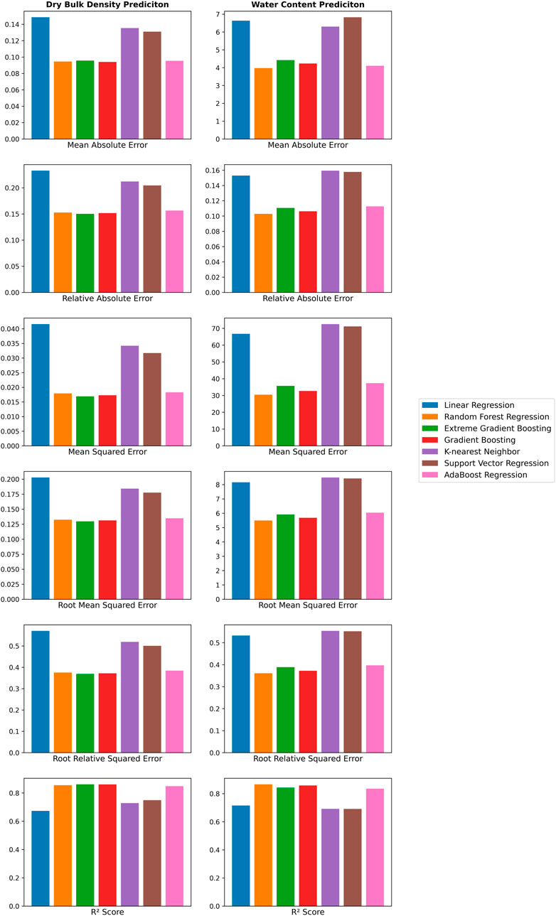
FIGURE 3. Visual representation of evaluation of seven regression methods for predicting dry bulk density and water content with metrics such as mean absolute error (MAE), relative absolute error (RAE), mean squared error (MSE), root mean squared error (RMSE), root relative squared error (RRSE), and R² score.

TABLE 2

TABLE 2. Summary of evaluation of regression methods for predicting dry bulk density and water content with metrics such as mean absolute error (MAE), relative absolute error (RAE), mean squared error (MSE), root mean squared error (RMSE), root relative squared error (RRSE), and R² score.

During the first predictions for DBD with the subset A1, we used the mean error between predicted WC versus measured WC as an additional measure of quality for all prediction methods. Table 3 summarizes the results across all prediction methods. In contrast to the previous test and training performance, Linear Regression performed with the smallest error (9.70%), while Random Forest Regression had the highest error (12.13%) amongst the methods.

TABLE 3

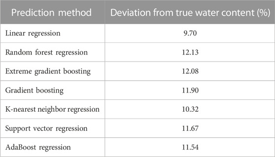
TABLE 3. Mean prediction error of water content across the seven prediction methods.

Before we could predict DBD for A2, we required a clay-silt pair for each of the 1790 data points in A2. Figure 4 shows the beta distributions for clay and silt based on the existing data across all datasets (Table 4). Clay content peaks between 10 and 20 percent, while silt content has its highpoint between 70 and 80 percent. We used random samples from these beta distributions with the subset A2 (Table 1) to estimate dry bulk density for all regression methods. To verify that model results were within a reasonable range and to allow comparison with the literature, we compared TOC values with measured and predicted DBD values. In Figure 5 we summarize the results obtained from the model predictions for Random Forest regression, Support Vector regression, and Linear Regression as well as measured values of TOC and dry bulk density. For completion, we show the results of the remaining four methods in the Supplementary Material (see Supplementary Figure S1).

FIGURE 4

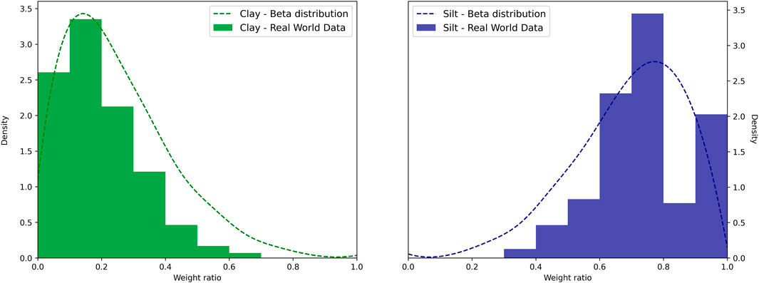
FIGURE 4. Derived beta distribution for clay (left, green dotted line) and silt (right, blue dotted line) from available grain size data.

TABLE 4

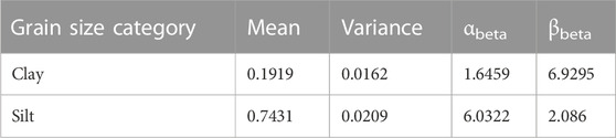
TABLE 4. Occurrence statistics within dataset of clay and silt and their calculated parameters α_beta and β_beta for the beta distribution.

FIGURE 5

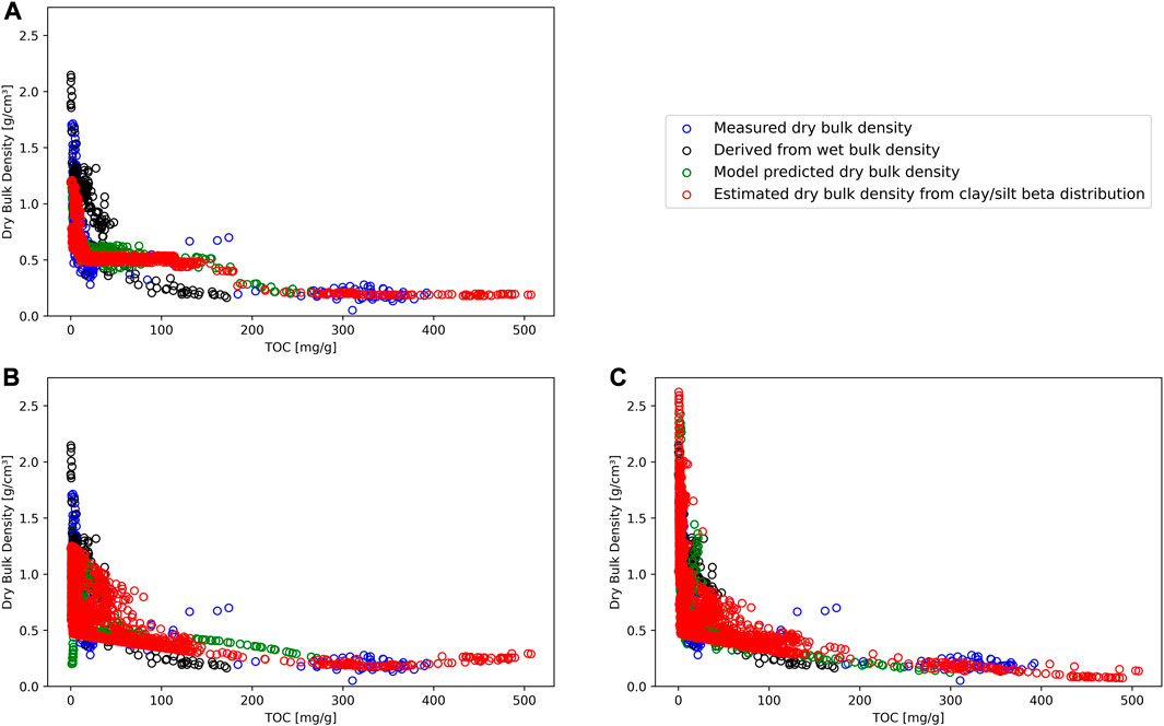
FIGURE 5. Model prediction results for dry bulk density against total organic carbon (TOC) for Random Forest regression (A), Support Vector regression (B), and Linear Regression (C). Directly measured dry bulk density (blue circles) and dry bulk density derived from measured wet bulk density (black circles) data are the same across all subplots. Green circles represents predicted dry bulk density values for each prediction method, where all input values were available. Red circles are estimated mean dry bulk density values for each prediction method with grain size data based on beta distribution for clay and silt.

In Figure 5A, the random forest regression displays a step-like curve with a plateau between about 20 and 150 mg·g⁻¹ TOC. Predicted values of dry bulk density ranged from 0.18 to 1.21 g·cm⁻³. We associated this pattern with potential overfitting, as the method ignores other measured values. Support Vector regression (Figure 5B) predicted values follow the measured values with a shallow increase from 300 to 500 mg·g⁻¹ TOC. DBD values for this method varied between 0.18 and 1.25 g·cm⁻³. The curve within Figure 5C (Linear regression) shows a similar log curve as presented in the literature, however, it exceeds the level of possible values [linear regression method maximum value: 4.06 g·cm⁻³; maximum physically possible value: 2.65 g·cm⁻³ (Avnimelech et al., 2001)]. The minimum value of this method was 0.07 g·cm⁻³. The exceeding values (n = 27) corresponded to deep level samples of core PG1341 (deeper than 15 m) where compactions plays a greater role than the method can reflect. To allow comparison with the literature, we excluded the values above 2.65 g·cm⁻³ from the linear model and continued with linear model further.

Figure 6 contains the comparison between mean OCAR and the temperature data from TraCE dataset for the 28 sediment cores. Some temperature data showed similarities as the core-drilling locations were in the same TraCE grid cell, e.g., EN18208 (Core No. 4—Lake Ilirney) and EN18218 (Core No. 5—Lake Rauchuvagytgyn), or PG2133 (Core No. 25—Lake Bolshoe Toko) and PG2208 (Core No. 27—Lake Bolshoe Toko). However, temperature ranges strongly varied within the dataset depending on the core location. For instance, for sediment core Tel 2006 (Core No. 28—Lake Teletskoye) we saw temperatures ranged from a minimum of −22.61°C to a maximum of 17.88°C, while temperatures for EN18218 (Core No. 5—Lake Rauchuvagytgyn) only spanned from −8.06°C to 2.60°C. Regarding OCAR values, we obtained the lowest overall values for PG1351 (Core No. 15—Lake El’gygytgyn) with a mean of 0.286 g·m⁻²·yr⁻¹ (uncertainty range max: 6.131 g·m⁻²·yr⁻¹, uncertainty range min: 0.008 g·m⁻²·yr⁻¹). We saw the highest OCAR value in ESM-1 (Core No. 6—East Sayan Mountains Lake) with 278 g·m⁻²·yr⁻¹, however, this value came with a large uncertainty range (min: 8.78 g·m⁻²·yr⁻¹, max: 3018.625 g·m⁻²·yr⁻¹). We calculated a mean OCAR of 24.615 g·m⁻²·yr⁻¹ for all collected sediment cores in our dataset.

FIGURE 6

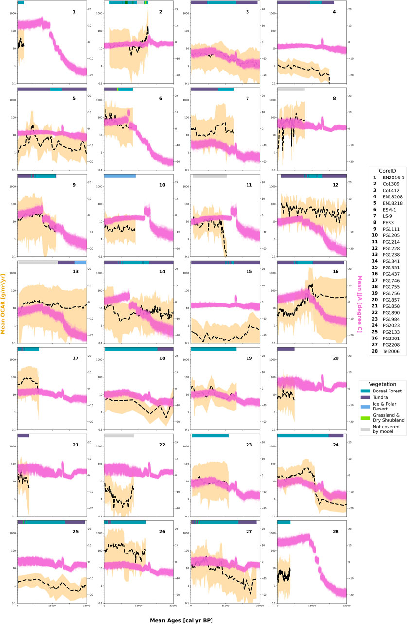
FIGURE 6. Organic carbon accumulation rate (mean values—black dashed line, 2σ uncertainty—golden shaded area) and June-July-August temperature from TraCE-21k temperature reconstruction (violet line) for the sediment cores used in this study (n = 28). Vegetation for each sediment core based on Dallmeyer et al. (2022) biome reconstruction.

Figure 7 contains two comparisons: on the left, a direct comparison between mean OCAR values and JJA temperature data across all sediment cores, while on the right is a comparison of z-transformed OCAR values over time. We obtained mean OCAR values for Last Glacial Maximum (9.47 g·m⁻²·yr⁻¹) and Last Deglaciation (10.53 g·m⁻²·yr⁻¹) at the lowest mean temperatures −12.75°C (range: −24.14°C to −0.51°C) and −10.62°C (range: −20.58°C to 2.12°C), respectively. We observed the highest temperature ranges in the Late Holocene with a mean temperature of 3.37°C (range: −12.69°C to 14.76°C), but only with a mean OCAR of 21.8 g·m⁻²·yr⁻¹. The highest OCAR values occurred in Bølling Allerød (38.07 g·m⁻²·yr⁻¹) and Early Holocene (40.68 g·m⁻²·yr⁻¹), where temperature ranged from −14.51°C to 1.69°C (mean value: −4.28°C) and −12.02°C to 8.20°C (mean value: −1.65°C), respectively.

FIGURE 7

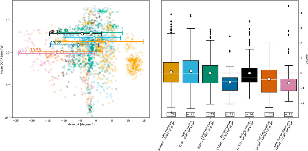
FIGURE 7. Left plot: Scatter plot showing the relationship between mean June-July-August (JJA) temperature and mean organic carbon accumulation rate (OCAR). For coloring, we have chosen the same color code as for the periods on the right. Vertical lines indicate the temperature range, while white dots show the mean temperature. Numbers on the left side of vertical lines are the overall mean OCAR for this period. Right plot: The OCAR z-scores grouped by the individual periods. The number below each box indicates the number of sediment cores contributing to this specific period. White dots are showing the overall mean z-scores, while the white lines are the overall median values. Black diamond markers represent outliers outside the 1.5 times interquartile range above the upper quartile and below the lower quartile.

However, when comparing the normalized data over time, we found that Mid-Holocene (mean z-score: 0.126, median z-score: −0.015) and Late Holocene (mean z-score: 0.089, median z-score: −0.055) were among the higher z-transformed OCAR values. Both Mid-Holocene and Late Holocene showed the highest temperature ranges, as shown on the left side of Figure 7. Periods that displayed a lower temperature range, i.e., Last Glacial Maximum, Last Deglaciation, and Younger Dryas, also revealed lower z-transformed OCAR values. Mean z-scores were −0.643, −0.402, and −0.616, while their median z-scores were −0.735, −0.429, and −0.577 for Last Glacial Maximum, Last Deglaciation, and Younger Dryas, respectively.

To check for correlation between temperature and OCAR, we first had to inspect visually Q-Q plots of those variables to check for normality (see Supplementary Figure S2). The visual inspection of the Q-Q plots, however, showed that variables were non-normal distributed. D'Agostino’s K² and Shapiro-Wilk test (Table 5) confirmed this numerically. We then determined the appropriate correlation coefficients for both variables untransformed, both variables z-transformed, and one where only OCAR was z-transformed while temperature was untransformed. Table 6 shows the correlation coefficients for Pearson, Spearman, Kendall-Tau, and Chatterjee, their p-value, and their statistical significance for the above cases. Except for Pearson correlation coefficient for both untransformed variables, all coefficient showed a statistical significance for the relationship between temperature and OCAR. Chatterjee coefficient displayed in all three cases a positive significance. Spearman’s rho value denoted a weak negative relationship (−0.06367) for untransformed values, while for z-transformed values it saw a weak positive relationship between temperature and OCAR (0.2394 and 0.0863).

TABLE 5

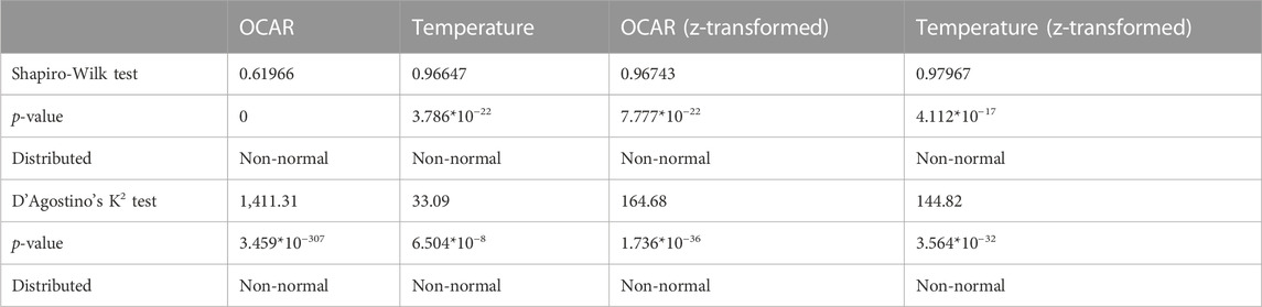
TABLE 5. Shapiro-Wilk and D’Agostino’s distribution results for OCAR and temperature as untransformed and z-transformed values.

TABLE 6

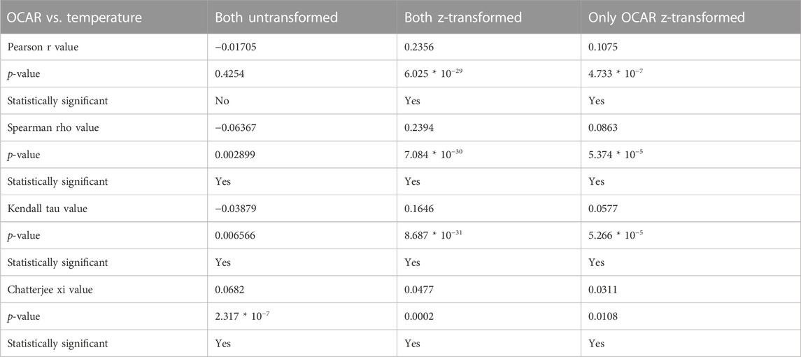
TABLE 6. Correlation statistic between OCAR and temperature using four different correlation techniques and an alpha value of 0.05 for the p-value.

4 Discussion

4.1 Lake carbon-temperature relationship across millennia

The Last Glacial Maximum (22,000 to 18,000 years BP) marks the lowest carbon accumulation in our observation period (9.47 g·m⁻²·yr⁻¹), followed by the Last Deglaciation (18,000 to 14,300 years BP—10.53 g·m⁻²·yr⁻¹) and Younger Dryas (12,700 to 11,700 years BP—17.22 g·m⁻²·yr⁻¹). Our finding suggest that lower OCAR values tend to occur in lower temperature ranges (Figure 7). Conversely, however, the highest temperatures did not directly result in the highest OCAR values, with the mean OCAR above 10°C being 5.97 g·m⁻²·yr⁻¹ (range 1.55–37.33 g·m⁻²·yr⁻¹). Even removing the cluster between 10°C and 15°C by excluding measurements from BN 2016-1 (Lake Bayan Nuur) and Tel 2006 (Lake Teletskoye) only slightly raises the mean OCAR values for the Late Holocene (present to 4,200 years BP) to 28.41 g·m⁻²·yr⁻¹.

The statistical analysis further supports this trend with only slight positive statistical significance between OCAR and temperature for our data collection (Table 6—see z-transformed values). However, both Bølling Allerød (14,300 to 12,700 years BP—38.07 g·m⁻²·yr⁻¹) and Early Holocene (11,700–8,200 years BP—40.68 g·m⁻²·yr⁻¹) are the two warm periods with the highest OCAR (see Figure 7), which also have the steepest gradients of temperature change (Rasmussen et al., 2006, 2014; Kaufman et al., 2020b). This may indicate that a rapid temperature change initiates a high accumulation of carbon in the lakes at the beginning of these warm phases and then decreases over time as the biological activity in the lakes increases.

However, our entire observation period was not covered by more than half of our collected sediment cores (n = 17), which partially limits the interpretation of individual sediment cores. Still we can identify numerous sediment cores (Co1309, Co1412, PG1111, PG1228, PG1238, and PG2208) that show a strong positive correlation (Pearson r-value above 0.5) between OCAR and temperature (see Supplementary Table S2). In particular, OCAR values for Co1412 (Lake Emanda) follow temperature variations throughout the observation period with the highest r-value of 0.8503.

We also observe synchrony with high r-values from the pair PG2133 and PG2208 (0.4599 and 0.5027, respectively) originating from the same lake (Lake Bolshoe Toko) but different positions within the lake. Similarly, the pair PG1755 and PG1756 (Lake Billyakh) show positive correlation with close individual r-values (0.3478 and 0.2341, respectively), but are not statistically significant with p-values greater than 0.05. In contrast, sediment cores PG1111 and PG1341 both come from Lake Lama but do not show a similar correlation with r-values of 0.8065 (PG1111) and 0.1813 (PG1341). The main difference from metadata perspective is that the first two pairs were part of the same expedition (Lake Billyakh—Yakutia 2005; Lake Bolshoe Toko—Yakutia 2013), whereas PG1111 (Norilsk/Taymyr 1993) and PG1341 (Norilsk 1997) are from two different expeditions of two different years. Therefore, even though they are from the same lake, comparing them may not be fair as the collection method of the sediment cores may have affected the results (Pfalz et al., 2021). The accuracy of laboratory analysis further improved over time between the retrievals of the two cores, which may have contributed to the observed differences in results.

Despite the complexity of individual limnological studies of lake systems, our collected dataset showed a positive correlation between OCAR and temperature with statistical significance for 11 out of 28 sediment cores. Even if there is a given heterogeneity amongst lake systems, we can conclude that temperature alone can explain OCAR variability within a lake. The 11 sediment cores are highly diverse and vary significantly in several aspects, as they share no common feature. They differ in location, vegetation surrounding the lakes, permafrost influence, catchment size, drilling distance from the shore, water depth at drilling site, lake area, lake volume, drilling device used, climate zone, and lake type. This would confirm our general understanding of the independence of the relationship between temperature as the sole driver and OCAR from other factors. However, the strength of the correlation depends both directly and indirectly on each contributing factor. Other environmental factors may weakened or amplified the strength of the temperature signal during our observation period. It is possible that temperature affected the remaining 17 cores, but local factors may have obscured the signal in the sediment.

Many of the processes known to influence the production and accumulation of organic carbon are subject to change due to modern climate warming (Larsen et al., 2011; Biskaborn et al., 2019). While understanding the long-term effects of temperature over thousands of years on OCAR is the main focus of our research, the short-term effects over couple hundred years can produce drastic results (Kastowski et al., 2011; Heathcote et al., 2015; Li et al., 2021). Many sediment cores in our collection (n = 21) have at least one surface sample pointing to the industrial era of the last 250 years (Toynbee, 1884). However, only six of those cores have more than two measurements, while only three (PG1111, PG2208, Tel 2006) have more than ten measurements. Because of this poor resolution, we do not have enough evidence to explain recent changes in OCARs. However, we have included these recent measurements in our Late Holocene samples to allow a comparison over a longer period.

Nevertheless, we must also consider the potential contribution of the modeled paleo-temperature and age determination data as an influencing factor in our interpretation. While the TraCE dataset provides an excellent tool for reconstruction, its development relied on global climate models that may not reflect the spatial variability required for our analysis. One solution would be the refinement of the reconstructed temperature through more local proxies and input parameters or downscaling of the TraCE dataset (Brown et al., 2020; Karger et al., 2023). Although LANDO is a more advanced age-depth modeling technique that combines multiple age-depth modeling software, it faces the same challenge as any other age-depth modeling software: Modeling software relies on age controls to establish an age-depth relationship. However, due to an insufficient number of age controls (cf. Blaauw et al., 2018) or greater uncertainty in the age determination data, a resulting age-depth model may not represent the exact absolute age. To circumvent this issue, we included the 2σ confidence intervals of these age-depth models and their resulting sedimentation rate in our OCAR calculations. We applied these intervals to the weighted mean age derived from four or five modeling software for every OCAR measurement. The consequence was an increase in the 2σ uncertainty intervals for each OCAR measurement, but overall a more accurate representation given the inherent uncertainty.

4.2 Spatial heterogeneity of lake carbon accumulation

For 11 sediment cores examined in our study we found statistical significance between OCAR and temperate, while the remaining sediment cores showed no such relationship, likely due to the complex nature of limnological studies and heterogeneity between lake systems. Given the spatial extent of our research, we must also consider unique local factors that may have affected the results. While we have sourced metadata and data sediment cores used in this study from published research articles (Table 1) that further provide in-depth analyses and interpretations, we will focus on three important unifying aspects: vegetation, permafrost, and geomorphology.

The vegetation reconstruction for around 21,000 years BP suggest that the oldest cores (n = 9) were mostly surrounded by tundra (Supplementary Table S3). The tundra biome is diverse and can present itself as an expansive landscape with mostly herbaceous plants, or as a mix of small trees and shrubs, such as Betula, Alnus, and Salix (Dallmeyer et al., 2022). The lack of significant abundance of evergreen trees—compared to boreal forests present in later reconstructions (11,700, 8,200, and 0 years BP—Figure 2)—may have contributed to the overall low carbon accumulation of lakes in the Last Deglaciation and Last Glacial Maximum.

To test this notion, we looked for sediment cores that remained in the same tundra biome throughout the entire vegetation reconstruction. We found that tundra vegetation surrounded one sediment cores (PG1351– Lake El’gygytgyn) for the longest time, with carbon accumulation rates averaging below 2.85 g·m⁻²·yr⁻¹ (mean value: 0.44 g·m⁻²·yr⁻¹). Melles et al. (2007) attribute the relatively low carbon content to the decomposition of organic matter due to the high oxygen content of the bottom water, but also a limited supply of terrestrial organic matter. The authors continue to determine a limited vegetation cover in the tundra-dominated catchment as main reason for the low carbon accumulation in the sediment (Melles et al., 2007).

In contrast, during the Bølling Allerød and Younger Dryas, most of the lake catchment areas in our data collection shift from tundra vegetation to boreal forests (Supplementary Table S3). Some even remain in boreal forest into the Late Holocene (n = 9), presumably fueled by the Holocene Thermal Maximum around 8,200 years BP (Kaufman et al., 2004; Wanner et al., 2015). Other catchment areas (EN18208, EN18218) transition back to tundra vegetation immediately at the end of the Younger Dryas, or at the end of the Early Holocene (LS-9, PG1228). OCAR values for sediment cores surrounded by boreal forest show strong variability in magnitude and incline. However, in most cases we observe an increase in OCAR values at the onset of higher vegetation cover, especially during warmer periods (Bølling Allerød, Early Holocene).

As an example of vegetation transition after the Younger Dryas, we looked at the lake catchment for sediment core PG1437 (Lake Lyadhej-To). There, the vegetation reconstruction indicates a transition from tundra to boreal forest at the beginning of the Early Holocene, which then lasted until the Late Holocene. Despite the Early Holocene being recognized as a warm period that allowed the boreal forest to expand northward (Tarasov et al., 2000; Anderson et al., 2010), our current data suggest that the carbon input from vegetation only affected the lake at the onset of the Early Holocene. Between 11,700 and 11,000 years BP mean OCAR increased to about 240 g·m⁻²·yr⁻¹, but then decreased to 39 g·m⁻²·yr⁻¹ around 8,200 years BP, with values even dropping to 12 g·m⁻²·yr⁻¹ at 7,700 years BP. The gradual northward expansion of boreal forests may have resulted in not fully established forests to provide an increased amount of organic carbon, which could explain the observed phenomenon for PG1437. However, this further supports our theory that a steep temperature gradient leads to more OCAR rather than sustained higher temperature.

While temperature is a major factor in vegetation change, we tested whether there is a direct relationship between OCAR and vegetation. The mean OCAR for lakes surrounded by boreal forest and tundra was 31.17 and 20.8 g·m⁻²·yr⁻¹, respectively. We saw the lowest mean OCAR in the “ice and polar dessert” biome with 5.3 g·m⁻²·yr⁻¹ and the highest mean OCAR in the “grassland and dry shrubland” biome with 50.17 g·m⁻²·yr⁻¹. However, we found no general correlation between mean OCAR and catchment vegetation in our data collection, with an r-value of only 0.047 (Supplementary Figure S3). A possible explanation for this might be a delayed vegetation response to a warming climate in the establishing phase of the boreal forest (Chapin and Starfield, 1997; Ernakovich et al., 2014; Zona et al., 2014). Following the reasoning of the dynamic vegetation module of JSBACH3 used in the vegetation reconstruction, we assume that trees live longer (up to 50 years) than grass (up to 1 year) (Dallmeyer et al., 2022). This would mean that as the trees grow, there would be less organic material available for transport to the lakes as they use their resources to grow. However, following the harmonization process by Dallmeyer et al. (2019), the grassland and dry shrubland biome has a similar minimum total vegetation coverage as the tundra biome, but differs by having more growing degree days, even as in boreal forest. This may indicate that vegetation with more growing days but short lifespans generally has a higher OCAR. We therefore have to assume that temperature drives both catchment vegetation and carbon accumulation in lakes, but at different times.

Despite the spatial heterogeneity of permafrost in the northern hemisphere (Mishra et al., 2021), our dataset contains a majority of cores (n = 26) located in areas with some degree of permafrost presence. Permafrost is perennially frozen ground that stays at or below 0°C for at least two consecutive years (French, 2007). Estimates of stored carbon within permafrost in the northern hemisphere range from around 1,460 to 1,600 PgC (petagrams of carbon, i.e., one billion metric tons of carbon) (Hugelius et al., 2014; Meredith et al., 2019; Schuur et al., 2022). Estimates by Lindgren et al. (2016) on the extent of permafrost during the Last Glacial Maximum suggest that permafrost had previously affected these areas as well. The two remaining sediment cores currently and previously unaffected by permafrost are Co1309 (Lake Ladoga) and PER3 (Lake Pernatoye). In addition, five sediment cores from our data collection originate from thermokarst lakes (Supplementary Table S1) that form as a direct result of permafrost thawing (Olefeldt et al., 2016).

Based on the mean OCAR, three sediment cores out of these five thermokarst lake cores (LS-9—Lake Dolgoe Ozero, PG1984—Lake Sysy-Kyuele, and PG2023—Lake Kyuntyunda) accumulate on average less than 60 g·m⁻²·yr⁻¹ (19.85, 9.92, and 24.78 g·m⁻²·yr⁻¹, respectively). The other two cores (PG1746—Lake Temje and PG2201—Lake Malaya Chabyda) show significantly higher values (62.31 and 129.58 g·m⁻²·yr⁻¹, respectively). Except for PG 1984 (min/max values: 2.98–18.75 g·m⁻²·yr⁻¹), the remaining cores are prone to strong fluctuations in OCAR in the minimum to maximum range:

1. PG2201: 20.64–275.04 g·m⁻²·yr⁻¹

2. PG1746: 13.26–89.3 g·m⁻²·yr⁻¹

3. LS-9: 8.3–52.74 g·m⁻²·yr⁻¹

4. PG 2023: 0.43–57.35 g·m⁻²·yr⁻¹

Compared to a global collection of OCAR values for lakes by Mendonça et al. (2017) (Figure 8), these fluctuation are still within the range of previously observed values. However, they do not indicate that the permafrost degradation process would directly contribute to a high OCAR in these lake types. The only exception being PG2201 (Lake Malaya Chabyda), where Hughes-Allen et al. (2021) associate the higher burial rates with increased bioproductivity in the lake. However, they also acknowledge that nutrient availability from the catchment, compact lake morphology, higher rates of sedimentation, and less exposure to warmer and oxygen-rich shallow waters further contributed to the higher OCAR values (Hughes-Allen et al., 2021). In the remaining cases, increased microbial activity may contribute to greater emission of greenhouse gases, resulting in less accumulation of carbon in the sediment (Serikova et al., 2019; in ’t Zandt et al., 2020).

FIGURE 8

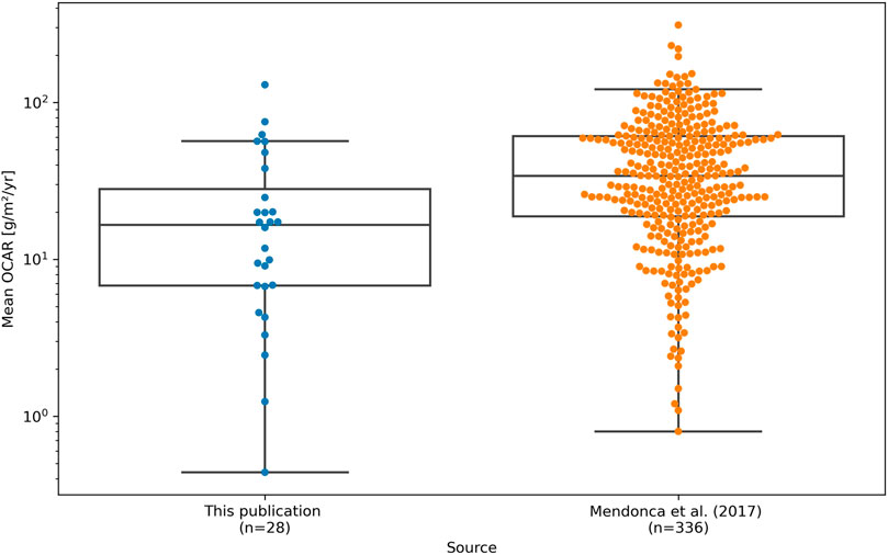
FIGURE 8. Comparison of mean OCAR values between lakes from our study (blue dots, left) and global lake compilation by Mendonça et al. (2017) (orange dots, right) with associated boxplots.

Lakes indirectly affected by permafrost, i.e., non-thermokarst lakes with permafrost in the catchment area, as well as lakes outside of permafrost zones show a similarly diverse picture. The uniqueness of a lake, given by its catchment area, lake volume and shape, its origin, and inflow parameters, can influence the carbon accumulation within the lake. Supplementary Table S1 summarizes the standard parameter of the lakes in our collection we were able to collect. However, when we looked at the correlation between OCAR and these lake-specific attributes, we found no correlation between them (Supplementary Figure S3). However, this shows the importance of limnological studies, as examining a wide variety of lakes would give us a better understanding of the accumulation process in Arctic lakes, since we cannot derive holistic statements from a limited number of lakes.

In this study, we primarily focused on the climatic impacts on lake sediment, which resulted in our assumptions partially overlooking the direct influence of microbial activity and oxygen levels in the water column. The limited availability of both current and historical data contributed to this situation. But given previous experiment (e.g., Li et al., 2017; Velthuis et al., 2018), we still assume that a temperature change has a direct influence on the microbial community. The effects of occurrence and interaction between different primary producers can contribute to a lead-lag relationship and needs further investigation when considering longer time scales. In meromictic lakes, the presence of low oxygen levels can create anaerobic/anoxic conditions affecting the in-lake carbon cycle, which in turn can skew the amount of deposited carbon. Obtaining additional sedimentological data on redox conditions is crucial for this analysis, but as many of the original studies did not include such data, we have to assume that oxygen levels in our lakes have changed on both short- and long-term basis. This means that future studies on individual lakes have the opportunity to link OCAR to redox conditions, providing further insight into the relationship between OCAR and microbial activity.

4.3 Method selection for predicting dry bulk density

Understanding the relationship between TOC and DBD has been essential in predicting DBD values. While we observed a logarithmic trend between values in our data collection (Supplementary Figure S4), the existing literature agreed that a log-linear model would best describe their relationship (Menounos, 1997; Dean and Gorham, 1998; Campbell et al., 2000; Avnimelech et al., 2001; Lan et al., 2015). However, we faced the challenge of high bulk density values occurring at low organic carbon values.

While low TOC values are common in northern lakes (Sobek et al., 2014), our log-linear model produced unrealistic DBD results, which exceeded physically possible values (Supplementary Figure S4). We found the highest DBD values in the deeper part of sediment core PG1341 at a depth of 1,461–1,883 cm, where compaction also most likely had a major impact on the material. We found that extrapolating given empirical equations from the literature to lower organic carbon values would result in a similar outcome (Supplementary Figure S4). To enable a more realistic representation, we assume that future models will have to take these special cases with different degrees of sediment compaction into account. We expect that a better understanding of the occurring compaction in sediment cores and its influence on the core composition will improve DBD predictions.

Due to the overestimation of dry bulk density for low TOC values of samples from deeper parts of sediment cores, and the apparent clustering of predicted values between 0 and 100 mg/g TOC, we considered several alternative prediction method to our log-linear model. As we evaluated these methods based on best-fit prediction metrics such as the R² score, we found that the supposedly best performing methods also showed signs of overfitting. Overfitting means that a model shows a strong bias towards seen data allowing only little room for variability for interpreting unseen data (Bilbao and Bilbao, 2017; Ying, 2019). Despite reducing the potential bias through cross validation, we found that the small size of available data mainly contributed to the overfitting in three cases (Random Forest Regression, Gradient Boosting, and Extreme Gradient Boosting). An increase in sample size could alleviate overfitting, as hyperparameter tuning produces more reliable results (Ying, 2019). However, in our case, having only 211 data points (80% of the total amount of training data points) available for hyperparameter tuning resulted in no visible improvements. We still assume that Random Forest Regression and Gradient Boosting methods have the potential to outperform log-linear models if more data is available. Other methods we tested may not be suitable for the prediction of water content and dry bulk density.

5 Conclusion

The purpose of the study was to determine whether there is connection between carbon accumulation in northern lakes and temperature changes that have occurred over the past 21,000 years. We found a slightly positive relationship between OCAR and temperature among our data collection, for which we generated more data using our log-linear model that superseded other data science techniques. While our dataset was diverse in terms of location, age of the sediment, permafrost areas, lake parameters, and catchment vegetation, we generally saw the highest OCAR values occurring during Bølling Allerød (14,300 to 12,700 years BP—38.07 g·m⁻²·yr⁻¹) and the Early Holocene (11,700–8,200 years BP—40.68 g·m⁻²·yr⁻¹). This could indicate that rapid warming events lead to high levels of carbon accumulation in lakes. As warming progresses, this effect appears to change with lower accumulation rates, presumably due to increased microbial activity triggering carbon dioxide and methane outgassing. While we achieved promising results with data from 28 sediment cores, more data from northern lakes would help us to build a greater level of confidence and accuracy on the matter.

Data availability statement

The datasets presented in this study can be found in online repositories. The names of the repository/repositories and accession number(s) can be found below: https://doi.org/10.5281/zenodo.7997700—Zenodo.

Author contributions

GP conceived the study, performed the analysis, and wrote the manuscript. BB, BD, and JCF supervised the works of GP. All authors contributed to the article and approved the submitted version.

Acknowledgments

The authors acknowledge the support of the Helmholtz Einstein Berlin International Berlin Research School in Data Science (HEIBRiDS), Alfred Wegener Institute—Helmholtz Center for Polar and Marine Research and its Open Access Publication Funds, Einstein Center Digital Future, and Humboldt University of Berlin. We thank Raphaël Hébert for the initial discussion about the TraCE-21k dataset and Alexander Rudolf for supporting the metadata collection. We thank the two reviewers whose comments and suggestions helped improve and clarify this manuscript.

Conflict of interest

The authors declare that the research was conducted in the absence of any commercial or financial relationships that could be construed as a potential conflict of interest.

Publisher’s note

All claims expressed in this article are solely those of the authors and do not necessarily represent those of their affiliated organizations, or those of the publisher, the editors and the reviewers. Any product that may be evaluated in this article, or claim that may be made by its manufacturer, is not guaranteed or endorsed by the publisher.

Supplementary material

The Supplementary Material for this article can be found online at: https://www.frontiersin.org/articles/10.3389/feart.2023.1233713/full#supplementary-material

References

Adams, H. E., Crump, B. C., and Kling, G. W. (2010). Temperature controls on aquatic bacterial production and community dynamics in arctic lakes and streams. Environ. Microbiol. 12, 1319–1333. doi:10.1111/j.1462-2920.2010.02176.x

PubMed Abstract | CrossRef Full Text | Google Scholar

Anderson, N. J., D’Andrea, W., and Fritz, S. C. (2009). Holocene carbon burial by lakes in SW Greenland. Glob. Chang. Biol. 15, 2590–2598. doi:10.1111/j.1365-2486.2009.01942.x

CrossRef Full Text | Google Scholar

Anderson, N. J., Heathcote, A. J., Engstrom, D. R., Ryves, D. B., Mills, K., Prairie, Y. T., et al. (2020). Anthropogenic alteration of nutrient supply increases the global freshwater carbon sink. Sci. Adv. 6, eaaw2145. doi:10.1126/sciadv.aaw2145

PubMed Abstract | CrossRef Full Text | Google Scholar

Anderson, P. M., Lozhkin, A. V., Solomatkina, T. B., and Brown, T. A. (2010). Paleoclimatic implications of glacial and postglacial refugia for Pinus pumila in western Beringia. Quat. Res. 73, 269–276. doi:10.1016/j.yqres.2009.09.008

CrossRef Full Text | Google Scholar

Anderson, P. M., Minyuk, P., Lozhkin, A., Cherepanova, M., Borkhodoev, V., and Finney, B. (2015). A multiproxy record of Holocene environmental changes from the northern Kuril Islands (Russian Far East). J. Paleolimnol. 54, 379–393. doi:10.1007/s10933-015-9858-y

CrossRef Full Text | Google Scholar

Andersson, L., Rantzer, A., and Beck, C. (1999). Model comparison and simplification. Int. J. Robust Nonlinear Control 9, 157–181. doi:10.1002/(SICI)1099-1239(199903)9:3<157::AID-RNC398>3.0.CO;2-8

CrossRef Full Text | Google Scholar

Andreev, A. A., Tarasov, P. E., Ilyashuk, B. P., Ilyashuk, E. A., Cremer, H., Hermichen, W.-D., et al. (2005). Holocene environmental history recorded in lake lyadhej-to sediments, polar urals, Russia. Palaeogeogr. Palaeoclimatol. Palaeoecol. 223, 181–203. doi:10.1016/j.palaeo.2005.04.004

CrossRef Full Text | Google Scholar

Asikainen, C. A., Francus, P., and Brigham-Grette, J. (2007). Sedimentology, clay mineralogy and grain-size as indicators of 65 ka of climate change from El’gygytgyn Crater Lake, Northeastern Siberia. J. Paleolimnol. 37, 105–122. doi:10.1007/s10933-006-9026-5

CrossRef Full Text | Google Scholar

Avnimelech, Y., Ritvo, G., Meijer, L. E., and Kochba, M. (2001). Water content, organic carbon and dry bulk density in flooded sediments. Aquac. Eng. 25, 25–33. doi:10.1016/S0144-8609(01)00068-1

CrossRef Full Text | Google Scholar

Ballinger, T. J., Overland, J. E., Wang, M., Bhatt, U. S., Hanna, E., Kim, S., et al. (2020). Arctic report card 2020: surface air temperature. The NOAA Arctic Report Card. doi:10.25923/gcw8-2z06

CrossRef Full Text | Google Scholar

Bartosiewicz, M., Przytulska, A., Lapierre, J. F., Laurion, I., Lehmann, M. F., and Maranger, R. (2019). Hot tops, cold bottoms: synergistic climate warming and shielding effects increase carbon burial in lakes. Limnol. Oceanogr. Lett. 4, 132–144. doi:10.1002/lol2.10117

CrossRef Full Text | Google Scholar

Bartsch, A., Hofler, A., Kroisleitner, C., and Trofaier, A. M. (2016). Land cover mapping in northern high latitude permafrost regions with satellite data: achievements and remaining challenges. Remote Sens. 8, 979. doi:10.3390/rs8120979

CrossRef Full Text | Google Scholar

Baumer, M. M., Wagner, B., Meyer, H., Leicher, N., Lenz, M., Fedorov, G., et al. (2021). Climatic and environmental changes in the Yana Highlands of north-eastern Siberia over the last c 57 000 years, derived from a sediment core from Lake Emanda. Boreas 50, 114–133. doi:10.1111/bor.12476

CrossRef Full Text | Google Scholar

Bilbao, I., and Bilbao, J. (2017). “Overfitting problem and the over-training in the era of data: particularly for artificial neural networks,” in 2017 Eighth International Conference on Intelligent Computing and Information Systems (ICICIS) (IEEE), Cairo, Egypt, 05-07 December 2017, 173–177. doi:10.1109/INTELCIS.2017.8260032

CrossRef Full Text | Google Scholar

Biskaborn, B. K., Forster, A., Pfalz, G., Pestryakova, L. A., Stoof-Leichsenring, K., Strauss, J., et al. (2023). Diatom responses and geochemical feedbacks to environmental changes at lake rauchuagytgyn (far east Russian arctic). Biogeosciences 20, 1691–1712. doi:10.5194/bg-20-1691-2023

CrossRef Full Text | Google Scholar

Biskaborn, B. K., Forster, A., Pfalz, G., Pestryakova, L. A., Strauss, J., Kröger, T., et al. (2022). Diatom responses and geochemical feedbacks to environmental changes at lake rauchuagytgyn (far east Russian arctic). EGUsphere 2022, 1–29. doi:10.5194/egusphere-2022-985

CrossRef Full Text | Google Scholar

Biskaborn, B. K., Herzschuh, U., Bolshiyanov, D., Savelieva, L., and Diekmann, B. (2012). Environmental variability in northeastern Siberia during the last ∼13,300yr inferred from lake diatoms and sediment-geochemical parameters. Palaeogeogr. Palaeoclimatol. Palaeoecol. 329–330, 22–36. doi:10.1016/j.palaeo.2012.02.003

PubMed Abstract | CrossRef Full Text | Google Scholar

Biskaborn, B. K., Nazarova, L., Kröger, T., Pestryakova, L. A., Syrykh, L. S., Pfalz, G., et al. (2021). Late quaternary climate reconstruction and lead-lag relationships of biotic and sediment-geochemical indicators at Lake Bolshoe Toko, siberia. Front. Earth Sci. 9, 1–22. doi:10.3389/feart.2021.737353

CrossRef Full Text | Google Scholar

Biskaborn, B. K., Smith, S. L., Noetzli, J., Matthes, H., Vieira, G., Streletskiy, D. A., et al. (2019). Permafrost is warming at a global scale. Nat. Commun. 10, 264. doi:10.1038/s41467-018-08240-4

PubMed Abstract | CrossRef Full Text | Google Scholar

Biskaborn, B. K., Subetto, D. A., Savelieva, L. A., Vakhrameeva, P. S., Hansche, A., Herzschuh, U., et al. (2016). Late quaternary vegetation and lake system dynamics in north-eastern siberia: implications for seasonal climate variability. Quat. Sci. Rev. 147, 406–421. doi:10.1016/j.quascirev.2015.08.014

CrossRef Full Text | Google Scholar

Blaauw, M., Christen, J. A., Bennett, K. D., and Reimer, P. J. (2018). Double the dates and go for Bayes — impacts of model choice, dating density and quality on chronologies. Quat. Sci. Rev. 188, 58–66. doi:10.1016/j.quascirev.2018.03.032

CrossRef Full Text | Google Scholar

Blaauw, M., and Christen, J. A. (2011). Flexible paleoclimate age-depth models using an autoregressive gamma process. Bayesian Anal. 6, 457–474. doi:10.1214/11-BA618

CrossRef Full Text | Google Scholar

Blaauw, M. (2010). Methods and code for “classical” age-modelling of radiocarbon sequences. Quat. Geochronol. 5, 512–518. doi:10.1016/j.quageo.2010.01.002

CrossRef Full Text | Google Scholar

Box, J. E., Colgan, W. T., Christensen, T. R., Schmidt, N. M., Lund, M., Parmentier, F. J. W., et al. (2019). Key indicators of arctic climate change: 1971-2017. Environ. Res. Lett. 14, 045010. doi:10.1088/1748-9326/aafc1b

CrossRef Full Text | Google Scholar

Brown, S. C., Wigley, T. M. L., Otto-Bliesner, B. L., and Fordham, D. A. (2020). StableClim, continuous projections of climate stability from 21000 BP to 2100 CE at multiple spatial scales. Sci. Data 7, 335–413. doi:10.1038/s41597-020-00663-3

PubMed Abstract | CrossRef Full Text | Google Scholar

Campbell, I. D., Campbell, C., Vitt, D. H., Kelker, D., Laird, L. D., Trew, D., et al. (2000). A first estimate of organic carbon storage in holocene lake sediments in Alberta, Canada. J. Paleolimnol. 24, 395–400. doi:10.1023/A:1008103605817

CrossRef Full Text | Google Scholar

Chapin, F. S., and Starfield, A. M. (1997). Time lags and novel ecosystems in response to transient climatic change in arctic Alaska. Clim. Change 35, 449–461. doi:10.1023/A:1005337705025

CrossRef Full Text | Google Scholar

Chatterjee, S. (2021). A new coefficient of correlation. J. Am. Stat. Assoc. 116, 2009–2022. doi:10.1080/01621459.2020.1758115

CrossRef Full Text | Google Scholar

Chen, T., and Guestrin, C. (2016). “XGBoost,” in Proceedings of the 22nd ACM SIGKDD International Conference on Knowledge Discovery and Data Mining, New York, NY, USA: ACM, 785–794. doi:10.1145/2939672.2939785

CrossRef Full Text | Google Scholar

Choudhary, S., Blaud, A., Osborn, A. M., Press, M. C., and Phoenix, G. K. (2016). Nitrogen accumulation and partitioning in a High Arctic tundra ecosystem from extreme atmospheric N deposition events. Sci. Total Environ. 554 (555), 303–310. doi:10.1016/j.scitotenv.2016.02.155

PubMed Abstract | CrossRef Full Text | Google Scholar

Clark, P. U., Dyke, A. S., Shakun, J. D., Carlson, A. E., Clark, J., Wohlfarth, B., et al. (2009). The last glacial maximum. Sci. (80) 325, 710–714. doi:10.1126/science.1172873

CrossRef Full Text | Google Scholar

Clow, D. W., Stackpoole, S. M., Verdin, K. L., Butman, D. E., Zhu, Z., Krabbenhoft, D. P., et al. (2015). Organic carbon burial in lakes and reservoirs of the conterminous United States. Environ. Sci. Technol. 49, 7614–7622. doi:10.1021/acs.est.5b00373

PubMed Abstract | CrossRef Full Text | Google Scholar

Courtin, J., Andreev, A. A., Raschke, E., Bala, S., Biskaborn, B. K., Liu, S., et al. (2021). Vegetation changes in southeastern siberia during the late Pleistocene and the holocene. Front. Ecol. Evol. 9, 233. doi:10.3389/fevo.2021.625096

CrossRef Full Text | Google Scholar

Cramer, W., Bondeau, A., Woodward, F. I., Prentice, I. C., Betts, R. A., Brovkin, V., et al. (2001). Global response of terrestrial ecosystem structure and function to CO2 and climate change: results from six dynamic global vegetation models. Glob. Chang. Biol. 7, 357–373. doi:10.1046/j.1365-2486.2001.00383.x

CrossRef Full Text | Google Scholar

Dallmeyer, A., Claussen, M., and Brovkin, V. (2019). Harmonising plant functional type distributions for evaluating Earth system models. Clim. Past. 15, 335–366. doi:10.5194/cp-15-335-2019

CrossRef Full Text | Google Scholar

Dallmeyer, A., Kleinen, T., Claussen, M., Weitzel, N., Cao, X., and Herzschuh, U. (2022). The deglacial forest conundrum. Nat. Commun. 13, 6035–6110. doi:10.1038/s41467-022-33646-6

PubMed Abstract | CrossRef Full Text | Google Scholar

Dask Development Team (2016). Dask: library for dynamic task scheduling. Available at: https://dask.org.

Google Scholar

Dean, W. E., and Gorham, E. (1998). Magnitude and significance of carbon burial in lakes, reservoirs, and peatlands. Geology 26, 535–538. doi:10.1130/0091-7613(1998)026<0535:MASOCB>2.3.CO;2

CrossRef Full Text | Google Scholar

Denfeld, B. A., Baulch, H. M., del Giorgio, P. A., Hampton, S. E., and Karlsson, J. (2018). A synthesis of carbon dioxide and methane dynamics during the ice-covered period of northern lakes. Limnol. Oceanogr. Lett. 3, 117–131. doi:10.1002/lol2.10079

CrossRef Full Text | Google Scholar

Diekmann, B., Pestryakova, L. A., Nazarova, L., Subetto, D. A., Tarasov, P. E., Stauch, G., et al. (2017). Late quaternary lake dynamics in the verkhoyansk mountains of eastern siberia: implications for climate and glaciation history. Polarforschung 86, 97–110. doi:10.2312/polarforschung.86.2.97

CrossRef Full Text | Google Scholar

Dolman, A. M. (2022). HAMSTR: hierarchical accumulation modelling with stan and R. Available at: https://github.com/EarthSystemDiagnostics/hamstr.

Google Scholar

Ebel, T., Melles, M., and Niessen, F. (1999). “Laminated sediments from levinson-lessing lake, northern central siberia - a 30,000 year record of environmental history?,” in Land-ocean systems in the siberian arctic: dynamics and history. H. Kassens, H. A. Bauch, I. A. Dmitrenko, H. Eicken, H.-W. Hubberten, and M. Melles Editors (Heidelberg: Springer Berlin), 425–436.

CrossRef Full Text | Google Scholar

Ernakovich, J. G., Hopping, K. A., Berdanier, A. B., Simpson, R. T., Kachergis, E. J., Steltzer, H., et al. (2014). Predicted responses of arctic and alpine ecosystems to altered seasonality under climate change. Glob. Chang. Biol. 20, 3256–3269. doi:10.1111/gcb.12568

PubMed Abstract | CrossRef Full Text | Google Scholar

Ferland, M. E., Prairie, Y. T., Teodoru, C., and Del Giorgio, P. A. (2014). Linking organic carbon sedimentation, burial efficiency, and long-term accumulation in boreal lakes. J. Geophys. Res. Biogeosciences 119, 836–847. doi:10.1002/2013JG002345

CrossRef Full Text | Google Scholar

French, H. M. (2007). The periglacial environment. Thrid. West Sussex, England: John Wiley & Sons Ltd. doi:10.1002/9781118684931

CrossRef Full Text | Google Scholar

Galloway, J. N., Dentener, F. J., Capone, D. G., Boyer, E. W., Howarth, R. W., Seitzinger, S. P., et al. (2004). Nitrogen cycles: past, present, and future. Biogeochemistry 70, 153–226. doi:10.1007/s10533-004-0370-0

CrossRef Full Text | Google Scholar

Greenacre, M. (2021). Compositional data analysis. Annu. Rev. Stat. Its Appl. 8, 271–299. doi:10.1146/annurev-statistics-042720-124436

CrossRef Full Text | Google Scholar

Gromig, R., Wagner, B., Wennrich, V., Fedorov, G., Savelieva, L., Lebas, E., et al. (2019). Deglaciation history of Lake Ladoga (northwestern Russia) based on varved sediments. Boreas 48, 330–348. doi:10.1111/bor.12379

CrossRef Full Text | Google Scholar

Gudasz, C., Bastviken, D., Steger, K., Premke, K., Sobek, S., and Tranvik, L. J. (2010). Temperature-controlled organic carbon mineralization in lake sediments. Nature 466, 478–481. doi:10.1038/nature09186

PubMed Abstract | CrossRef Full Text | Google Scholar

Gudasz, C., Sobek, S., Bastviken, D., Koehler, B., and Tranvik, L. J. (2015). Temperature sensitivity of organic carbon mineralization in contrasting lake sediments. J. Geophys. Res. Biogeosciences 120, 1215–1225. doi:10.1002/2015JG002928

CrossRef Full Text | Google Scholar

Guillemette, F., von Wachenfeldt, E., Kothawala, D. N., Bastviken, D., and Tranvik, L. J. (2017). Preferential sequestration of terrestrial organic matter in boreal lake sediments. J. Geophys. Res. Biogeosciences 122, 863–874. doi:10.1002/2016JG003735

CrossRef Full Text | Google Scholar

Hammer, K. J., Kragh, T., and Sand-Jensen, K. (2019). Inorganic carbon promotes photosynthesis, growth, and maximum biomass of phytoplankton in eutrophic water bodies. Freshw. Biol. 64, 1956–1970. doi:10.1111/fwb.13385

CrossRef Full Text | Google Scholar

Harris, C. R., Millman, K. J., van der Walt, S. J., Gommers, R., Virtanen, P., Cournapeau, D., et al. (2020). Array programming with NumPy. Nature 585, 357–362. doi:10.1038/s41586-020-2649-2

PubMed Abstract | CrossRef Full Text | Google Scholar

Harwart, S., Hagedorn, B., Melles, M., and Wand, U. (1999). Lithological and biochemical properties in sediments of Lama Lake as indicators for the late Pleistocene and Holocene ecosystem development of the southern Taymyr Peninsula, Central Siberia. Boreas 28, 167–180. doi:10.1111/j.1502-3885.1999.tb00212.x

CrossRef Full Text | Google Scholar

Haslett, J., and Parnell, A. C. (2008). A simple monotone process with application to radiocarbon-dated depth chronologies. J. R. Stat. Soc. Ser. C Appl. Stat. 57, 399–418. doi:10.1111/j.1467-9876.2008.00623.x

CrossRef Full Text | Google Scholar

He, F. (2011). Simulating transient climate evolution of the last deglaciation with CCSM3. Boulder, Colorado: University Corporation for Atmospheric Research.

Google Scholar

Head, M. J., Pillans, B., Zalasiewicz, J. A., Alloway, B., Beu, A. G., Cohen, K. M., et al. (2021). Formal ratification of subseries for the Pleistocene series of the quaternary system. Episodes 44, 241–247. doi:10.18814/epiiugs/2020/020084

CrossRef Full Text | Google Scholar

Heathcote, A. J., Anderson, N. J., Prairie, Y. T., Engstrom, D. R., and del Giorgio, P. A. (2015). Large increases in carbon burial in northern lakes during the Anthropocene. Nat. Commun. 6, 10016. doi:10.1038/ncomms10016

PubMed Abstract | CrossRef Full Text | Google Scholar

Hein, M. (1997). Inorganic carbon limitation of photosynthesis in lake phytoplankton. Freshw. Biol. 37, 545–552. doi:10.1046/j.1365-2427.1997.00180.x

CrossRef Full Text | Google Scholar

Hoff, U., Biskaborn, B. K., Dirksen, V. G., Dirksen, O., Kuhn, G., Meyer, H., et al. (2015). Holocene environment of central kamchatka, Russia: implications from a multi-proxy record of two-yurts lake. Glob. Planet. Change 134, 101–117. doi:10.1016/j.gloplacha.2015.07.011

CrossRef Full Text | Google Scholar

Hoff, U., Dirksen, O., Dirksen, V., Herzschuh, U., Hubberten, H.-W., Meyer, H., et al. (2012). Late Holocene diatom assemblages in a lake-sediment core from Central Kamchatka, Russia. J. Paleolimnol. 47, 549–560. doi:10.1007/s10933-012-9580-y

CrossRef Full Text | Google Scholar

Hoff, U., Dirksen, O., Dirksen, V., Kuhn, G., Meyer, H., and Diekmann, B. (2014). Holocene freshwater diatoms: palaeoenvironmental implications from south kamchatka, Russia. Boreas 43, 22–41. doi:10.1111/bor.12019

CrossRef Full Text | Google Scholar

Hollis, J. M., Hannam, J., and Bellamy, P. H. (2012). Empirically-derived pedotransfer functions for predicting bulk density in European soils. Eur. J. Soil Sci. 63, 96–109. doi:10.1111/j.1365-2389.2011.01412.x

CrossRef Full Text | Google Scholar

Huang, Z., and Laffan, S. W. (2009). Sensitivity analysis of a decision tree classification to input data errors using a general Monte Carlo error sensitivity model. Int. J. Geogr. Inf. Sci. 23, 1433–1452. doi:10.1080/13658810802634949

CrossRef Full Text | Google Scholar

Hugelius, G., Strauss, J., Zubrzycki, S., Harden, J. W., Schuur, E. A. G., Ping, C. L., et al. (2014). Estimated stocks of circumpolar permafrost carbon with quantified uncertainty ranges and identified data gaps. Biogeosciences 11, 6573–6593. doi:10.5194/bg-11-6573-2014

CrossRef Full Text | Google Scholar

Hughes-Allen, L., Bouchard, F., Hatté, C., Meyer, H., Pestryakova, L. A., Diekmann, B., et al. (2021). 14,000-year carbon accumulation dynamics in a siberian lake reveal catchment and lake productivity changes. Front. Earth Sci. 9, 1–19. doi:10.3389/feart.2021.710257

CrossRef Full Text | Google Scholar

in ’t Zandt, M. H., Liebner, S., and Welte, C. U. (2020). Roles of thermokarst lakes in a warming world. Trends Microbiol. 28, 769–779. doi:10.1016/j.tim.2020.04.002

PubMed Abstract | CrossRef Full Text | Google Scholar

Joblib Development Team (2020). JOBLIB: running Python functions as pipeline jobs. Available at: https://joblib.readthedocs.io/.

Google Scholar

Karger, D. N., Nobis, M. P., Normand, S., Graham, C. H., and Zimmermann, N. E. (2023). CHELSA-TraCE21k - high-resolution (1 km) downscaled transient temperature and precipitation data since the Last Glacial Maximum. Clim. Past. 19, 439–456. doi:10.5194/cp-19-439-2023

CrossRef Full Text | Google Scholar

Kastowski, M., Hinderer, M., and Vecsei, A. (2011). Long-term carbon burial in European lakes: analysis and estimate. Glob. Biogeochem. Cycles 25, 1–12. doi:10.1029/2010GB003874

CrossRef Full Text | Google Scholar

Kaufman, D. S., Ager, T. A., Anderson, N. J., Anderson, P. M., Andrews, J. T., Bartlein, P. J., et al. (2004). Holocene thermal maximum in the western Arctic (0 - 180° W). Quat. Sci. Rev. 23, 529–560. doi:10.1016/j.quascirev.2003.09.007

CrossRef Full Text | Google Scholar

Kaufman, D. S., McKay, N. P., Routson, C. C., Erb, M. P., Davis, B. A. S., Heiri, O., et al. (2020a). A global database of Holocene paleotemperature records. Sci. Data 7, 115–134. doi:10.1038/s41597-020-0445-3

PubMed Abstract | CrossRef Full Text | Google Scholar

Kaufman, D. S., McKay, N. P., Routson, C., Erb, M. P., Dätwyler, C., Sommer, P. S., et al. (2020b). Holocene global mean surface temperature, a multi-method reconstruction approach. Sci. Data 7, 201–213. doi:10.1038/s41597-020-0530-7

PubMed Abstract | CrossRef Full Text | Google Scholar

Klump, J. V., Edgington, D. N., Granina, L., and Remsen, C. C. (2020). Estimates of the remineralization and burial of organic carbon in Lake Baikal sediments. J. Gt. Lakes. Res. 46, 102–114. doi:10.1016/j.jglr.2019.10.019

CrossRef Full Text | Google Scholar

Kluyver, T., Ragan-Kelley, B., Pérez, F., Granger, B., Bussonnier, M., Frederic, J., et al. (2016). “Jupyter Notebooks -- a publishing format for reproducible computational workflows,” in Positioning and power in academic publishing: players, agents and agendas. Editors F. Loizides, and B. Schmidt (IOS Press), 87–90. doi:10.3233/978-1-61499-649-1-87

CrossRef Full Text | Google Scholar

Kuang, X., Schenk, F., Smittenberg, R., Hällberg, P., and Zhang, Q. (2021). Seasonal evolution differences of east Asian summer monsoon precipitation between Bølling-Allerød and younger Dryas periods. Clim. Change 165, 19. doi:10.1007/s10584-021-03025-z

CrossRef Full Text | Google Scholar

Lan, J., Xu, H., Liu, B., Sheng, E., Zhao, J., and Yu, K. (2015). A large carbon pool in lake sediments over the arid/semiarid region, NW China. Chin. J. Geochem. 34, 289–298. doi:10.1007/s11631-015-0047-5

CrossRef Full Text | Google Scholar

Larsen, S., Andersen, T., and Hessen, D. O. (2011). Climate change predicted to cause severe increase of organic carbon in lakes. Glob. Chang. Biol. 17, 1186–1192. doi:10.1111/j.1365-2486.2010.02257.x

CrossRef Full Text | Google Scholar

Li, Q., Gogo, S., Leroy, F., Guimbaud, C., and Laggoun-Défarge, F. (2021). Response of peatland CO2 and CH4 fluxes to experimental warming and the carbon balance. Front. Earth Sci. 9, 1–13. doi:10.3389/feart.2021.631368

CrossRef Full Text | Google Scholar

Li, Z., He, L., Zhang, H., Urrutia-Cordero, P., Ekvall, M. K., Hollander, J., et al. (2017). Climate warming and heat waves affect reproductive strategies and interactions between submerged macrophytes. Glob. Chang. Biol. 23, 108–116. doi:10.1111/gcb.13405

PubMed Abstract | CrossRef Full Text | Google Scholar

Lindgren, A., Hugelius, G., Kuhry, P., Christensen, T. R., and Vandenberghe, J. (2016). GIS-Based maps and area estimates of northern hemisphere permafrost extent during the last glacial maximum. Permafr. Periglac. Process 27, 6–16. doi:10.1002/ppp.1851

CrossRef Full Text | Google Scholar

Lougheed, B. C., and Obrochta, S. P. (2019). A rapid, deterministic age-depth modeling routine for geological sequences with inherent depth uncertainty. Paleoceanogr. Paleoclimatology 34, 122–133. doi:10.1029/2018PA003457

CrossRef Full Text | Google Scholar

Lozhkin, A., Anderson, P. M., Minyuk, P., Korzun, J., Brown, T., Pakhomov, A., et al. (2018). Implications for conifer glacial refugia and postglacial climatic variation in western Beringia from lake sediments of the Upper Indigirka basin. Boreas 47, 938–953. doi:10.1111/bor.12316

CrossRef Full Text | Google Scholar

Lozhkin, A. V., Anderson, P. M., Matrosova, T. V., and Minyuk, P. S. (2007). The pollen record from El’gygytgyn lake: implications for vegetation and climate histories of northern chukotka since the late middle Pleistocene. J. Paleolimnol. 37, 135–153. doi:10.1007/s10933-006-9018-5

CrossRef Full Text | Google Scholar

Lu, Y., Biswas, A., Wen, M., and Si, B. (2021). Predicting bulk density in deep unsaturated soils based on multiple scale decomposition. Geoderma 385, 114859. doi:10.1016/j.geoderma.2020.114859

CrossRef Full Text | Google Scholar

Mackay, A. W., Bezrukova, E. V., Leng, M. J., Meaney, M., Nunes, A., Piotrowska, N., et al. (2012). Aquatic ecosystem responses to Holocene climate change and biome development in boreal, central Asia. Quat. Sci. Rev. 41, 119–131. doi:10.1016/j.quascirev.2012.03.004

CrossRef Full Text | Google Scholar

Martín, M. Á., Reyes, M., and Taguas, F. J. (2017). Estimating soil bulk density with information metrics of soil texture. Geoderma 287, 66–70. doi:10.1016/j.geoderma.2016.09.008

CrossRef Full Text | Google Scholar

Mathews, G. M., and Vial, J. (2017). Overcoming model simplifications when quantifying predictive uncertainty, 1–37. Available at: http://arxiv.org/abs/1703.07198.

Google Scholar

Melles, M., Brigham-Grette, J., Glushkova, O. Y., Minyuk, P. S., Nowaczyk, N. R., and Hubberten, H.-W. (2007). Sedimentary geochemistry of core PG1351 from Lake El’gygytgyn-a sensitive record of climate variability in the East Siberian Arctic during the past three glacial-interglacial cycles. J. Paleolimnol. 37, 89–104. doi:10.1007/s10933-006-9025-6

CrossRef Full Text | Google Scholar

Melles, M., Brigham-Grette, J., Minyuk, P. S., Nowaczyk, N. R., Wennrich, V., DeConto, R. M., et al. (2012). 2.8 Million years of arctic climate change from Lake El’gygytgyn, NE Russia. Sci. (80) 337, 315–320. doi:10.1126/science.1222135

PubMed Abstract | CrossRef Full Text | Google Scholar

Mendonça, R., Müller, R. A., Clow, D., Verpoorter, C., Raymond, P., Tranvik, L. J., et al. (2017). Organic carbon burial in global lakes and reservoirs. Nat. Commun. 8, 1694–1696. doi:10.1038/s41467-017-01789-6

PubMed Abstract | CrossRef Full Text | Google Scholar

Menounos, B. (1997). The water content of lake sediments and its relationship to other physical parameters: an alpine case study. Holocene 7, 207–212. doi:10.1177/095968369700700208

CrossRef Full Text | Google Scholar

Meredith, M., Sommerkorn, M., Cassotta, S., Derksen, C., Ekaykin, A., Hollowed, A., et al. (2019). “Polar regions,” in IPCC special report on the ocean and cryosphere in a changing climate. H.-O. Pörtner, D. C. Roberts, V. Masson-Delmotte, P. Zhai, M. Tignor, and E. Poloczanska Editors (Cambridge, UK: Cambridge Univ Press), 203–320.

Google Scholar

Middelboe, M., and Lundsgaard, C. (2003). Microbial activity in the Greenland sea: role of DOC lability, mineral nutrients and temperature. Aquat. Microb. Ecol. 32, 151–163. doi:10.3354/ame032151

CrossRef Full Text | Google Scholar

Mishra, U., Hugelius, G., Shelef, E., Yang, Y., Strauss, J., Lupachev, A., et al. (2021). Spatial heterogeneity and environmental predictors of permafrost region soil organic carbon stocks. Sci. Adv. 7, eaaz5236–13. doi:10.1126/sciadv.aaz5236

PubMed Abstract | CrossRef Full Text | Google Scholar

Nazarova, L., Lüpfert, H., Subetto, D. A., Pestryakova, L. A., and Diekmann, B. (2013). Holocene climate conditions in central Yakutia (Eastern Siberia) inferred from sediment composition and fossil chironomids of Lake Temje. Quat. Int. 290–291, 264–274. doi:10.1016/j.quaint.2012.11.006

PubMed Abstract | CrossRef Full Text | Google Scholar

Obu, J., Westermann, S., Bartsch, A., Berdnikov, N., Christiansen, H. H., Dashtseren, A., et al. (2019). Northern Hemisphere permafrost map based on TTOP modelling for 2000–2016 at 1 km2 scale. Earth-Science Rev. 193, 299–316. doi:10.1016/j.earscirev.2019.04.023

CrossRef Full Text | Google Scholar

Olefeldt, D., Goswami, S., Grosse, G., Hayes, D., Hugelius, G., Kuhry, P., et al. (2016). Circumpolar distribution and carbon storage of thermokarst landscapes. Nat. Commun. 7, 13043. doi:10.1038/ncomms13043

PubMed Abstract | CrossRef Full Text | Google Scholar

Palladino, M., Romano, N., Pasolli, E., and Nasta, P. (2022). Developing pedotransfer functions for predicting soil bulk density in Campania. Geoderma 412, 115726. doi:10.1016/j.geoderma.2022.115726

CrossRef Full Text | Google Scholar

Parnell, A. C., Haslett, J., Allen, J. R. M., Buck, C. E., and Huntley, B. (2008). A flexible approach to assessing synchroneity of past events using Bayesian reconstructions of sedimentation history. Quat. Sci. Rev. 27, 1872–1885. doi:10.1016/j.quascirev.2008.07.009

CrossRef Full Text | Google Scholar

Pearson, R. G., Phillips, S. J., Loranty, M. M., Beck, P. S. A., Damoulas, T., Knight, S. J., et al. (2013). Shifts in Arctic vegetation and associated feedbacks under climate change. Nat. Clim. Chang. 3, 673–677. doi:10.1038/nclimate1858

CrossRef Full Text | Google Scholar

Pedregosa, F., Varoquaux, G., Gramfort, A., Michel, V., Thirion, B., Grisel, O., et al. (2012). Scikit-learn: machine learning in Python. 10.1007/s13398-014-0173-7.2.

Google Scholar

Peng, B., Wang, G., Ma, J., Leong, M. C., Wakefield, C., Melott, J., et al. (2018). SoS notebook: an interactive multi-language data analysis environment. Bioinformatics 34, 3768–3770. doi:10.1093/bioinformatics/bty405

PubMed Abstract | CrossRef Full Text | Google Scholar

Pfalz, G., Diekmann, B., Freytag, J.-C., and Biskaborn, B. K. (2021). Harmonizing heterogeneous multi-proxy data from lake systems. Comput. Geosci. 153, 104791. doi:10.1016/j.cageo.2021.104791

CrossRef Full Text | Google Scholar

Pfalz, G., Diekmann, B., Freytag, J.-C., Syrykh, L. S., Subetto, D. A., and Biskaborn, B. K. (2022). Improving age–depth relationships by using the LANDO (“Linked age and depth modeling”) model ensemble. Geochronology 4, 269–295. doi:10.5194/gchron-4-269-2022

CrossRef Full Text | Google Scholar

Qin, L., Lin, L., Ding, S., Yi, C., Chen, J., and Tian, Z. (2022). Evaluation of pedotransfer functions for predicting particle density of soils with low organic matter contents. Geoderma 416, 115812. doi:10.1016/j.geoderma.2022.115812

CrossRef Full Text | Google Scholar

Raab, A., Melles, M., Berger, G. W., Hagedorn, B., and Hubberten, H.-W. (2003). Non-glacial paleoenvironments and the extent of weichselian ice sheets on severnaya zemlya, Russian high arctic. Quat. Sci. Rev. 22, 2267–2283. doi:10.1016/S0277-3791(03)00139-2

CrossRef Full Text | Google Scholar

Rasmussen, S. O., Andersen, K. K., Svensson, A. M., Steffensen, J. P., Vinther, B. M., Clausen, H. B., et al. (2006). A new Greenland ice core chronology for the last glacial termination. J. Geophys. Res. Atmos. 111, D06102. doi:10.1029/2005JD006079

CrossRef Full Text | Google Scholar

Rasmussen, S. O., Bigler, M., Blockley, S. P., Blunier, T., Buchardt, S. L., Clausen, H. B., et al. (2014). A stratigraphic framework for abrupt climatic changes during the last glacial period based on three synchronized Greenland ice-core records: refining and extending the INTIMATE event stratigraphy. Quat. Sci. Rev. 106, 14–28. doi:10.1016/j.quascirev.2014.09.007

CrossRef Full Text | Google Scholar

Rebba, R., Mahadevan, S., and Huang, S. (2006). Validation and error estimation of computational models. Reliab. Eng. Syst. Saf. 91, 1390–1397. doi:10.1016/j.ress.2005.11.035

CrossRef Full Text | Google Scholar

Roiha, T., Peura, S., Cusson, M., and Rautio, M. (2016). Allochthonous carbon is a major regulator to bacterial growth and community composition in subarctic freshwaters. Sci. Rep. 6, 34456. doi:10.1038/srep34456

PubMed Abstract | CrossRef Full Text | Google Scholar

Rudaya, N. A., Nazarova, L., Frolova, L., Palagushkina, O., Soenov, V., Cao, X., et al. (2021). The link between climate change and biodiversity of lacustrine inhabitants and terrestrial plant communities of the Uvs Nuur Basin (Mongolia) during the last three millennia. Holocene 31, 095968362110190. doi:10.1177/09596836211019093

CrossRef Full Text | Google Scholar

Rudaya, N. A., Nazarova, L., Novenko, E., Andreev, A. A., Kalugin, I., Daryin, A., et al. (2016). Quantitative reconstructions of mid-to late Holocene climate and vegetation in the north-eastern Altai mountains recorded in Lake Teletskoye. Glob. Planet. Change 141, 12–24. doi:10.1016/j.gloplacha.2016.04.002

CrossRef Full Text | Google Scholar

Sadeghi, B. (2022). Chatterjee correlation coefficient: a robust alternative for classic correlation methods in geochemical studies- (including “TripleCpy” Python package). Ore Geol. Rev. 146, 104954. doi:10.1016/j.oregeorev.2022.104954

CrossRef Full Text | Google Scholar

Schuur, E. A. G., Abbott, B. W., Commane, R., Ernakovich, J. G., Euskirchen, E. S., Hugelius, G., et al. (2022). Permafrost and climate change: carbon cycle feedbacks from the warming arctic. Annu. Rev. Environ. Resour. 16, 343–371. doi:10.1146/annurev-environ-012220-011847

CrossRef Full Text | Google Scholar

Seabold, S., and Perktold, J. (2010). “statsmodels: econometric and statistical modeling with python,” in 9th Python in Science Conference.

CrossRef Full Text | Google Scholar

Serikova, S., Pokrovsky, O. S., Laudon, H., Krickov, I. V., Lim, A. G., Manasypov, R. M., et al. (2019). High carbon emissions from thermokarst lakes of Western Siberia. Nat. Commun. 10, 1552–1557. doi:10.1038/s41467-019-09592-1

PubMed Abstract | CrossRef Full Text | Google Scholar

Sharma, S., Blagrave, K., Magnuson, J. J., O’Reilly, C. M., Oliver, S., Batt, R. D., et al. (2019). Widespread loss of lake ice around the Northern Hemisphere in a warming world. Nat. Clim. Chang. 9, 227–231. doi:10.1038/s41558-018-0393-5

CrossRef Full Text | Google Scholar

Sharma, S., Meyer, M. F., Culpepper, J., Yang, X., Hampton, S., Berger, S. A., et al. (2020). Integrating perspectives to understand lake ice dynamics in a changing world. J. Geophys. Res. Biogeosciences 125, 1–18. doi:10.1029/2020JG005799

CrossRef Full Text | Google Scholar

Sobek, S., Anderson, N. J., Bernasconi, S. M., and Del Sontro, T. (2014). Low organic carbon burial efficiency in arctic lake sediments. J. Geophys. Res. Biogeosciences 119, 1231–1243. doi:10.1002/2014JG002612

CrossRef Full Text | Google Scholar

Sundqvist, M. K., Liu, Z., Giesler, R., and Wardle, D. A. (2014). Plant and microbial responses to nitrogen and phosphorus addition across an elevational gradient in subarctic tundra. Ecology 95, 1819–1835. doi:10.1890/13-0869.1

PubMed Abstract | CrossRef Full Text | Google Scholar

Tarasov, P. E., Volkova, V. S., Webb, T., Guiot, J., Andreev, A. A., Bezusko, L. G., et al. (2000). Last glacial maximum biomes reconstructed from pollen and plant macrofossil data from northern Eurasia. J. Biogeogr. 27, 609–620. doi:10.1046/j.1365-2699.2000.00429.x

CrossRef Full Text | Google Scholar

Tchebakova, N. M., Parfenova, E., and Soja, A. J. (2009). The effects of climate, permafrost and fire on vegetation change in Siberia in a changing climate. Environ. Res. Lett. 4, 045013. doi:10.1088/1748-9326/4/4/045013

CrossRef Full Text | Google Scholar

Toynbee, A. (1884). The industrial revolution. Beacon Press Available at: https://books.google.co.uk/books?id=NU0VeWQSrKYC.

Google Scholar

Velthuis, M., Kosten, S., Aben, R., Kazanjian, G., Hilt, S., Peeters, E. T. H. M., et al. (2018). Warming enhances sedimentation and decomposition of organic carbon in shallow macrophyte-dominated systems with zero net effect on carbon burial. Glob. Chang. Biol. 24, 5231–5242. doi:10.1111/gcb.14387

PubMed Abstract | CrossRef Full Text | Google Scholar

Virtanen, P., Gommers, R., Oliphant, T. E., Haberland, M., Reddy, T., Cournapeau, D., et al. (2020). SciPy 1.0: fundamental algorithms for scientific computing in Python. Nat. Methods. 17, 261–272. doi:10.1038/s41592-019-0686-2

PubMed Abstract | CrossRef Full Text | Google Scholar

von Hippel, B., Stoof-Leichsenring, K. R., Schulte, L., Seeber, P., Biskaborn, B. K., Diekmann, B., et al. (2021). Long-term fungus–plant co-variation from multi-site sedimentary ancient DNA metabarcoding in Siberia. 10.1101/2021.11.05.465756.

Google Scholar

Vuglinsky, V., and Valatin, D. (2018). Changes in ice cover duration and maximum ice thickness for rivers and lakes in the asian part of Russia. Nat. Resour. 09, 73–87. doi:10.4236/nr.2018.93006

CrossRef Full Text | Google Scholar

Vyse, S. A., Herzschuh, U., Andreev, A. A., Pestryakova, L. A., Diekmann, B., Armitage, S. J., et al. (2020). Geochemical and sedimentological responses of arctic glacial Lake Ilirney, chukotka (far east Russia) to palaeoenvironmental change since ∼51.8 ka BP. Quat. Sci. Rev. 247, 106607. doi:10.1016/j.quascirev.2020.106607

CrossRef Full Text | Google Scholar

Vyse, S. A., Herzschuh, U., Pfalz, G., Pestryakova, L. A., Diekmann, B., Nowaczyk, N., et al. (2021). Sediment and carbon accumulation in a glacial lake in chukotka (arctic siberia) during the late Pleistocene and holocene: combining hydroacoustic profiling and down-core analyses. Biogeosciences 18, 4791–4816. doi:10.5194/bg-18-4791-2021

CrossRef Full Text | Google Scholar

Wagner, B., and Melles, M. (2008). A Holocene seabird record from Raffles Sø sediments, East Greenland, in response to climatic and oceanic changes. Boreas 30, 228–239. doi:10.1111/j.1502-3885.2001.tb01224.x

CrossRef Full Text | Google Scholar

Wagner, B., Melles, M., Hahne, J., Niessen, F., and Hubberten, H.-W. (2000). Holocene climate history of geographical society Ø, east Greenland — Evidence from Lake sediments. Palaeogeogr. Palaeoclimatol. Palaeoecol. 160, 45–68. doi:10.1016/S0031-0182(00)00046-8

CrossRef Full Text | Google Scholar

Walker, M., Gibbard, P., Head, M. J., Berkelhammer, M., Björck, S., Cheng, H., et al. (2019). Formal subdivision of the holocene series/epoch: a summary. J. Geol. Soc. India 93, 135–141. doi:10.1007/s12594-019-1141-9

CrossRef Full Text | Google Scholar

Walther, G., Post, E., Convey, P., Menzel, A., Parmesank, C., Beebee, T. J. C., et al. (2002). Ecological responses to recent climate change. Nature 416, 389–395. doi:10.1038/416389a

PubMed Abstract | CrossRef Full Text | Google Scholar

Wanner, H., Wanner, H., Mercolli, L., Mercolli, L., Grosjean, M., Grosjean, M., et al. (2015). Holocene climate variability and change; a data-based review. J. Geol. Soc. Lond. 172, 254–263. doi:10.1144/jgs2013-101

CrossRef Full Text | Google Scholar

Windirsch, T., Grosse, G., Ulrich, M., Forbes, B. C., Göckede, M., Wolter, J., et al. (2022). Large herbivores on permafrost— A pilot study of grazing impacts on permafrost soil carbon storage in northeastern siberia. Front. Environ. Sci. 10, 1–17. doi:10.3389/fenvs.2022.893478

CrossRef Full Text | Google Scholar

Wolfe, B. B., Edwards, T. W. D., Aravena, R., Forman, S. L., Warner, B. G., Velichko, A. A., et al. (2000). Holocene paleohydrology and paleoclimate at treeline, north-central Russia, inferred from oxygen isotope records in lake sediment cellulose. Quat. Res. 53, 319–329. doi:10.1006/qres.2000.2124

CrossRef Full Text | Google Scholar

Ying, X. (2019). An overview of overfitting and its solutions. J. Phys. Conf. Ser. 1168, 022022. doi:10.1088/1742-6596/1168/2/022022

CrossRef Full Text | Google Scholar

Zona, D., Lipson, D. A., Richards, J. H., Phoenix, G. K., Liljedahl, A. K., Ueyama, M., et al. (2014). Delayed responses of an arctic ecosystem to an extreme summer: impacts on net ecosystem exchange and vegetation functioning. Biogeosciences 11, 5877–5888. doi:10.5194/bg-11-5877-2014

CrossRef Full Text | Google Scholar

Zwart, J. A., Hanson, Z. J., Read, J. S., Fienen, M. N., Hamlet, A. F., Bolster, D., et al. (2019). Cross-scale interactions dictate regional lake carbon flux and productivity response to future climate. Geophys. Res. Lett. 46, 8840–8851. doi:10.1029/2019GL083478

CrossRef Full Text | Google Scholar