 Jie Nie1
 Weiyang Wang
94% of researchers rate our articles as excellent or good
Learn more about the work of our research integrity team to safeguard the quality of each article we publish.
Find out more
ORIGINAL RESEARCH article
Front. Earth Sci., 22 August 2023
Sec. Environmental Informatics and Remote Sensing
Volume 11 - 2023 | https://doi.org/10.3389/feart.2023.1230470
This article is part of the Research TopicUnderstanding of Big Data and Artificial Intelligence in Promoting the Environmental GovernanceView all 6 articles
The accumulation of liquid in shale gas wells will lead to an increase in bottom-hole pressure, and a decrease in production, even the shutdown of gas wells. Accurately predicting the variation of liquid height in shale gas wellbore and the corresponding production is helpful to determine the liquid accumulation status and the development of reasonable drainage construction plans. It can provide theoretical support for the efficient and stable production of shale gas wells. A predictive analysis model of shale gas wellbore liquid accumulation was established based on a liquid film carrying model, which considers the coupling of flow in the reservoir and wellbore in shale gas production system. This model can accurately predict the liquid accumulation height, production rate, and the bottomhole pressure changes in liquid-accumulating gas wells. A comparative analysis was conducted on the effect of wellbore structure on liquid accumulation characteristics in the typical upward-type and downward-type horizontal wells in the W block. In upward-type horizontal wells, the liquid height increases slowly before the liquid accumulation fills the horizontal section, and the liquid height increases rapidly after the liquid accumulation fills the horizontal section. Compared to upward-type horizontal wells, the liquid height rises more quickly and the gas production rate is more sensitive to liquid accumulation in downward-type horizontal wells.
Shale reservoirs are tight and usually require hydraulic fracturing to achieve economic development (Vincent, 2012; Zhou et al., 2016). Working condition data shows that cumulative liquid production only accounts for 10%–50% of the fracturing fluid, and a large amount of unrecovered fracturing fluid remains in the reservoir, causing serious damage to the gas reservoir (Haluszczak et al., 2013). During the production of shale gas wells, unrecovered fracturing fluid flows out of the formation with gas and is produced to the surface through the wellbore. In the later stage of gas well production, as the formation pressure depletes and gas production decreases, some liquid droplets and film flow reversely in the wellbore, and cannot be completely carried to the surface. The liquid phase falls back and accumulates at the bottom of the well, forming a liquid accumulation. After liquid accumulation occurs at the bottom of the well, a complex multiphase flow is formed in the production formation and tubing, increasing the pressure drop and forming greater back pressure on the gas reservoir, which seriously affects the production of gas wells and can even cause water lock. Microwave irradiation can improve the desorption rate of adsorbed gas and remove the water-lock effect (Liu et al., 2023). Additionally, microwave irradiation may induce micro-cracking in the shale matrix, which may improve matrix permeability. However, this is a complex process and was not considered in this study. Timely diagnosis of liquid accumulation in gas wells and calculation of liquid accumulation height, as well as taking measures to prevent fluid accumulation in advance, can reduce the damage of liquid accumulation to the gas reservoir, which is of great significance to ensure the efficient production of gas wells.
The calculation of liquid accumulation in wellbore involves two models: the liquid-carrying critical flow rate model and the liquid accumulation prediction model. The liquid-carrying critical model mainly considers the critical state of liquid-carrying production rate in gas wells, and there are four typical model: liquid droplet model, liquid film model, minimum pressure drop model, and gas well stability analysis model. The liquid droplet model was firstly proposed by Turner et al. in vertical wells, which is one of the most widely used models in current applications. It assumes that the liquid droplets in wellbore are spherical, and provides a critical liquid carrying model suitable for mist flow regimes with high producing gas-liquid ratio (Ilobi and Ikoku, 1981). Belfroid et al. modified the Turner model to account for the influence of wellbore inclination angle on the critical liquid carrying velocity (Stefan et al., 2008).
The liquid film model analyses the liquid film attached on the pipe wall and believes that the reverse flow of the liquid film is the cause of liquid accumulation at the bottom of the wellbore. If the gas flow velocity in the wellbore is high enough to lift the liquid film, then there will be no liquid accumulation at the bottom of the well. Wallis et al. firstly proposed a criterion to judge the reversal of the liquid film which was based on dimensionless gas flow rate according to their research (Wallis, 1969).
The minimum pressure drop model assumes that the critical liquid carrying flow velocity corresponds to the gas velocity at which the pressure gradient in the wellbore is minimum. When the gas velocity is lower than this critical velocity, liquid accumulation will occur in the wellbore (Shen et al., 2019a). Yuan et al. demonstrated that liquid accumulation begins to occur at the bottom of the pipe when the pressure gradient in the wellbore reaches its minimum value through experimental observations and data analysis (Yuan et al., 2013).
The gas well stability analysis model considers that the accumulation of liquid in gas wells is related to production stability. And the production rate determined by the nodal system analysis method at the stable production point of the gas well is considered the critical gas rate for liquid removal (Zhang et al., 2019). Greene et al. used the coupling of tubing outflow curve and formation productivity equation for gas well stability analysis, and they take the inflection point on the curve of wellbore pressure drop with gas production as the minimum production value for stable flow, that is, the stable flow points (Greene, 1983). Pagan et al. proposed a transient model to predict gas well liquid loading, which considered the gas production rate when the inflow and outflow curves are tangent as the critical gas carrying capacity (Pagan and Waltrich, 2016).
Currently, the prediction models of the liquid accumulation level in gas well mainly include the method considering difference between tubing head pressure and casing head pressure (Gou, 2006; Yang et al., 2011; Xiong et al., 2015; Gaol and Valko, 2016), node analysis method, (Li and Yong, 2001; Du et al., 2004; Lea and Nickens, 2004; Zhang and Chen, 2008; Garcia et al., 2016; Sousa et al., 2017), and coupling analysis method on wellbore flow and reservoir seepage (Li et al., 2011; Tie, 2012; Li et al., 2018). The coupling method requires the combination of gas-liquid pressure drop in tubing, producing gas liquid ratio, critical liquid carrying flow rate, productivity equation of gas, and gas pressure drop in casing. This method is mostly in line with the principle of liquid accumulation in gas wells, and some scholars have also conducted relevant research on multiphase flow in liquid loading gas wells based on the coupling of gas-liquid flow in reservoirs and wellbores. Han et al. established a model and solution method for the coupling of reservoir seepage and horizontal wellbore flow in fractured horizontal gas wells, taking into account the properties and equation of state of the real gas. They also analyzed the impact of factors such as wellbore radius, length of horizontal wellbore, number of fractures, and pipe wall roughness on pressure drop in wellbore and gas well productivity (Han et al., 2002). Sun et al. developed a production prediction model and its solution method for hydraulic fractured horizontal wells in low-permeability gas reservoirs, by coupling gas seepage in the formation with the flow in the wellbore based on the properties of the gas (Sun et al., 2005). Hao et al. proposed a mathematical model to calculate the production rate in liquid loading gas wells, considering the productivity equations for Darcy flow, non-Darcy flow, and the skin effect in liquid producing gas wells (Hao et al., 2006). Li et al. derived a coupled model between the horizontal well and gas reservoir for single-phase steady-state flow and investigated the influence of factors such as wellbore diameter on the productivity of horizontal gas wells (Li et al., 2010). Schiferli et al. analyzed the effect of the interaction between the wellbore and reservoir on the liquid accumulation in gas wells (Schiferli et al., 2010). Riza et al. analyzed the factors affecting the critical liquid carrying rate and liquid accumulation in gas wells, they combined the gas well productivity equation with the pressure drop and heat transfer model of gas-liquid mixture in the wellbore and the critical liquid carrying model together, and found that the well productivity index and diameter were the key factors (Riza et al., 2016). Tang et al. established a coupled model of wellbore flow and horizontal well productivity by considering the flow in reservoirs and the hydraulic fracturing of horizontal wells, and sensitivity analysis was also conducted on the coupled model (Tang, 2019).
The accumulation of liquid at the bottom in gas wells can affect the gas well productivity and further impact gas well dewatering. Prediction liquid accumulation performance in wellbore during gas well production is a major challenge. In addition, the timing to unload liquid in gas wells with liquid accumulation has a significant impact on gas well stable production. If liquid removal is delayed, the accumulation of liquid at the bottom of the well reduces the total gas production and decreases the recovery of the gas field. If liquid removal measures are implemented too early, it leads to waste of funds and affects the normal production of gas wells (Yang, 1994). Therefore, it is crucial to predict the growth behavior of liquid accumulation height in gas wells to determine a reasonable timing for liquid removal. However, to the authors’ knowledge, the problem mentioned above has not yet been effectively solved. This research established a transient model for multiphase flow in wellbore during liquid accumulation, considering the reservoir production capacity and liquid-carrying capacity of gas. The relevant calculation programs were built, and the change in liquid accumulation height and flowing bottomhole pressure of shale gas wells were predicted effectively.
When the production rate of a gas well is lower than the critical liquid-carrying flow rate, liquid phase will accumulate from the bottomhole of the well (Zhou, 2014; Liang et al., 2015). The typical wellbore fluid accumulation process is shown in Figure 1. In the early stage of production, the formation pressure is high enough, and the liquid produced from the formation is carried to the wellhead by the gas in the form of droplets and liquid films, and no fluid accumulates at the bottom of the well. However, as the gas well continues to be developed, the pressure of the formation decreases. When the gas flow rate in the wellbore is less than the critical flow rate, it is not possible to carry all the produced liquid to the wellhead, and some of the liquid accumulates at the bottom of the wellbore, forming fluid accumulation. With the increase of liquid accumulation, the height of liquid accumulation in the wellbore continues to increase, forming a complex multiphase flow in the production layer and wellbore, and the pressure loss in the wellbore increases, resulting in a rapid decline in gas well production and weakening of the natural flowing ability of the gas well. In addition, liquid accumulated in bottomhole will damage the gas layer, form a certain back pressure on the gas reservoir, and even kill the gas reservoir, resulting in the complete stop of natural flowing of the gas well (Turner et al., 1969; Ilobi and Ikoku, 1981; Guo et al., 2005; Van Gool and Currie, 2008).
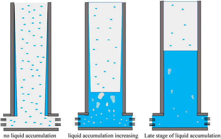
FIGURE 1. Schematic of the liquid accumulation process in gas wells.
In the early stage of wellbore liquid accumulation, the natural flowing ability of the gas well is weakened, but gas phase still has a certain liquid-carrying ability, and part of the formation liquid can still be carried to the wellhead by gas, and the wellhead produces gas and water simultaneously. As shown in Figure 2, gas-liquid two-phase flow flows from the liquid surface to the wellhead, and the formation produced fluid is carried to the wellhead in the form of droplets or liquid films. The section from the bottomhole to the liquid surface is the flow of gas passing through the liquid column. Compared with the gas flow, the liquid flow is relatively small. When calculating the pressure drop in this section, it can be regarded as a two-phase flow with zero net liquid flow.
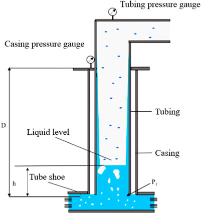
FIGURE 2. Flow state in the wellbore after liquid accumulation in the gas well.
Assumptions.
1) The liquid produced from the formation is water.
2) The gas-liquid ratio of formation output is constant.
3) Formation pressure is constant.
4) Liquid has begun to accumulate in the bottom, but the well is not locked.
5) The flow pattern in the wellbore is annular mist flow.
The dynamic prediction model for height of liquid accumulated in wellbore can be divided into two parts: pressure profile calculation and liquid loading calculation. The pressure profile calculation mainly includes gas-liquid two-phase flow section above the liquid level of wellbore accumulation and zero-net liquid flow two-phase flow section below the liquid level. The calculation of liquid loading mainly includes the calculation of wellbore carrying capacity and the calculation of liquid rate supplied form the formation.
When gas wells experience liquid loading, according to the pressure balance relationship, there is:
Where pwf is the bottomhole pressure, MPa; pt is the tubing pressure at wellhead, MPa; Δp1 is the pressure drop from the wellhead to the liquid level, and Δp2 is the pressure drop from the liquid level to the bottom of the well.
1) Calculation of pressure profile in liquid loading gas wells
The bottomhole pressure (Δp1) is calculated using the pressure gradient equation for gas-liquid flow, and for well sections which wellbore inclination angles less than 45°, the Hagedorn-Brown method is used (Hagedorn and Brown, 1965).
Where Δp is the total pressure drop of the gas-water mixture in the wellbore section, Pa; Δz is the length of the calculation section, m;
For well sections which wellbore inclination angles greater than 45°, the Beggs-Brill method is used for calculation (Beggs and Brill, 1973).
Where Hl is the liquid holdup, which is the volume fraction of the liquid phase in the calculation section; θ is the angle between the pipeline and the horizontal direction, degree; G is the mass flow rate, kg/s; v is the average velocity of the mixture, m/s; ρl is liquid density, kg/m; ρg is gas density, kg/m; p is the pressure of the calculation section, Pa; vsg is the gas phase superficial velocity, m/s.
2) Calculation of Two-Phase Flow for Zero Net Liquid Flow Rate
The calculation for Δp2 is performed using a model for the zero net liquid flow rate two-phase flow (Liu and Zhou, 2002; Liu et al., 2009; We et al., 2009). Below the liquid accumulation level in the tubing, the flow pattern appears as either slug flow or bubble flow, and the pressure gradient is determined by the gravity of the gas-liquid mixture as well as the frictional resistance between the mixture and the pipe wall.
Where ρm is density of the gas-water mixture in the wellbore section, kg/m3. The mixture density can be obtained by weighting the gas and liquid phase densities by the holdup across the tubing cross-section.
The friction factor between the mixture and pipe wall can still be calculated using a relevant formula.
Where Rem is the mixture Reynolds number, μl is the liquid phase viscosity, Pa⋅s.
The holdup rate Hl can be calculated using the drift flux model.
Where C0 is the velocity distribution coefficient, vd is the drift velocity of gas, m/s.
The drift velocity of the gas phase in slug flow follows the Harmathy’s correlation for the rise velocity of small bubbles in stagnant liquid (Harmathy, 1960).
Where σ is the surface tension, N/m.
The drift velocity of the gas phase in plug flow follows the Bendiksen’s correlation for the rise velocity of Taylor bubbles in stagnant liquid (Bendiksen, 1984).
When the transition from slug flow to bubble flow occurs at gas void fraction is 0.25 (the liquid holdup is 0.75) (Liu et al., 2017).
The critical liquid-carrying flow rate of gas can be calculated using the liquid film model as follows: based on the minimum shear stress theory and the critical flow rate model of annular mist flow, it is assumed that there is no liquid droplet entrainment and the liquid film is uniformly distributed around the gas core. The dimensionless expression for the shear stress at the annular flow interface is given by (Shen et al., 2019b):
Where τI is the interfacial shear stress, Pa;
The interface shear stress is a function of dimensionless liquid film thickness
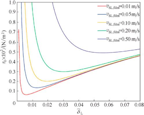
FIGURE 3. Schematic of relationship between interface shear stress and dimensionless liquid film thickness in vertical pipe.
Where the friction factor f1 at the gas-liquid interface is calculated using the relationship given by Shekhar et al.
The critical flow rate to remove the liquid under standard conditions is:
Where qscr is the critical flow rate, m3/d; A is the section area of tubing, m2; Z is the gas compressibility factor; T is the temperature, K.
Gas productivity can be calculated by binomial equation or exponential equation. Formation liquid production is a function of gas production [ql = f (qg)], so the current liquid flow rate from the formation into the wellbore is calculated based on the gas-liquid ratio.
1) Binomial productivity equation
When the gas flows at high speed, the inertial and turbulent effects become very significant, which is no longer fit with Darcy’s law. Forchheimer (1901) proposed a second order modification of Darcy’s linear seepage equation for this situation:
Where μ is the viscosity of gas, Pa.s; k is the permeability, m2; u is the velocity, m/s; ρ is the density, kg/m3; β is the coefficient of velocity, m-1.
The second term at the right side of the above equation reflects the turbulent inertia effect of high-speed seepage flow. For gas wells, the pressure difference method is adopted:
Where pr is the formation pressure, Pa; pwf is the flowing bottomhole pressure, Pa; qsc is gas production rate at the standard condition, m3/d. The coefficient a and b can be can be determined through data fitting based on well testing data.
2) Exponential equation
In the case of full laminar flow, the production formula of gas well stable flow is:
Where h is the thickness of the formation, m; re is the drainage radius, m; rw is the wellbore radius,m; S is the skin factor.
In the case of high speed non-Darcy flow in gas Wells, turbulent effect will increase the flow resistance, and the production will decrease under the same pressure difference. To reflect the presence of turbulence, gas well production is represented by an exponential formula as follows:
When n=1, it means complete laminar flow; when n=0.5, it means very severe turbulence. The coefficient c and n can also be determined through data fitting based on well testing data.
The prediction process of liquid accumulation height change in gas well is as Figure 4:
1) Calculate the initial liquid level location;
2) Calculate liquid production at the current time according to gas production;
3) Calculate the amount of liquid carried in the wellbore in the current state;
4) The amount of liquid accumulated in wellbore and the variation of liquid height are calculated according to the amount of liquid produced at the current time and the amount of liquid carried in wellbore;
5) The bottomhole pressure at the next time is calculated according to the change of fluid accumulation height;
6) Based on the new bottomhole pressure, gas production and liquid production at the next moment can be calculated according to the two-phase productivity equation of gas production and liquid production;
7) Repeat(3) ∼ (6)until the number of cycles i reaches the set value n;
8) Realize the dynamic prediction of wellbore state, output the height of liquid accumulation, gas production rate, liquid production rate, bottomhole flow pressure changes with time.
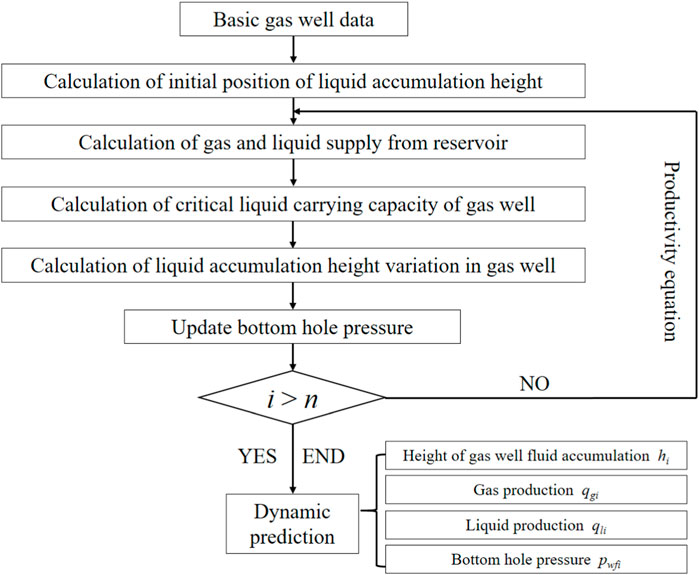
FIGURE 4. Prediction process of gas well fluid accumulation height change.
The model assumes that liquid loading has already occurred in the wellbore, the initial state of the wellbore including the current liquid accumulation height needs to be calculated first. The calculation method is as follows: The pressure at the liquid level and bottomhole can be obtained based on the measured pressure profile from wellhead to bottomhole. In the absence of liquid level data, the liquid level position can be obtained by calculating the liquid accumulation height using liquid holdup model in gas wellbore (You et al., 2016; Meng et al., 2019). First, the flowing bottomhole pressure pwf is calculated based on the productivity Equation 20 and used as the initial value. The pressure drop calculation method for two-phase flow with zero net liquid flow (4–11) is used to calculate the pressure profile below the liquid level (Curve B). Meanwhile, the gas-liquid two-phase flow Equations 2, 3 are used to calculate the pressure profile above the liquid level with the wellhead pressure pt as the initial value (Curve A). The two curves are plotted on the same coordinate system, and the value corresponding to the intersection point is the depth of the wellbore liquid level. The wellbore liquid accumulation height h is then calculated, as shown in Figure 5.
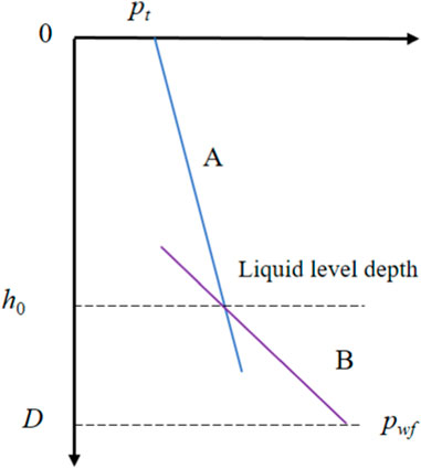
FIGURE 5. Schematic of wellbore liquid height calculation.
Based on the model for predicting changes of liquid accumulation height in the wellbore, a computational program was developed using a programming language-Python. The program was used to perform example calculations and analysis in the W block.
Due to the influence of formation dip angle, there are two types of horizontal wellbore shapes for shale gas horizontal wells in the W block: upturned sloping horizontal wells and downturned sloping horizontal wells. Due to the difference in wellbore dip angle, different gas-liquid flow patterns will appear in the horizontal section, exhibiting different liquid accumulation characteristics. The W-1# well was fractured and put into production on 11 November 2018, using a 139.7 mm casing for initial production. The wellhead test pressure was 13.02 MPa and the test production rate was 24.72×10⁴ m3/d. In August 2019, fluctuations in production rate began to occur, indicating liquid accumulation. On 20 July 2020, a 60.3 mm tubing was installed for production. The horizontal section of W-1# well is a downturned sloping horizontal section, while the horizontal section of W-2# well is an upturned horizontal section. The specific well depth structure is shown in Figure 6.
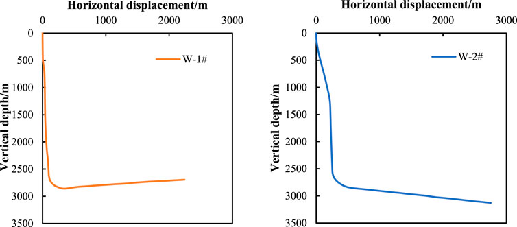
FIGURE 6. Schematic of well body structure of W-1# and W-2# wells.
After a vertical depth of 2873.23 m in W-1# well, the wellbore upturned, and the average inclination angle was 95° (95° from the vertical direction and −5° from the horizontal direction). The total length of the wellbore was 4905 m. The target A had a measured depth of 3205.00 m and a vertical depth of 2845.41 m; the target B had a measured depth of 4905.00 m and a vertical depth of 2711.44 m. The wellbore upturned at point C (measured depth 3029.68 m, vertical depth 2873.23 m), which is the lowest point of the horizontal section. After a vertical depth of 2880 m in W-2# well, the average inclination angle was 82° (82° from the vertical direction and +8° from the horizontal direction), and the total length of the wellbore was 5250 m, with a horizontal section length of 2200 m. The target A had a measured depth of 3050 m and a vertical depth of 2867.59 m; the B target had a measured depth of 5250 m and a vertical depth of 3143.17 m, which is the lowest point of the horizontal section.
Taking W-1# and W-2# wells as examples, the formation pressure is 12 MPa, the gas productivity index is 180 m3/(d⋅MPa), the flowing pressure at the end of the horizontal section is 8.3 MPa, and the producing gas-liquid ratio is 13800 sm3/m3, the prediction and analysis of liquid accumulation performance were carried out, and the liquid accumulation height changes are shown in Figure 7.
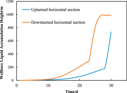
FIGURE 7. Changes in the height of effusion between upturned and downturned horizontal sections.
The early stage liquid accumulation height increases slowly for both upturned sloping and downturned sloping horizontal wells during the liquid accumulation process. After the horizontal section is completely filled with liquid, the liquid accumulation height increases rapidly until the gas well is completely locked.
For downturned horizontal wells, liquid accumulation continuously gathers from the toe of the horizontal section, and creates a certain backpressure on the reservoir, resulting in a decrease in gas well production. Additionally, when the liquid fills the entire horizontal section, the liquid accumulation height relative to the lowest point of the wellbore reaches 275.58m, and the flow regime in the horizontal section is either bubbly flow or slug flow. The fluid flow in the horizontal section needs to overcome the static pressure head of the liquid accumulation, resulting in a greater impact on the pressure profile in the horizontal section and gas well production during the liquid accumulation process, and causes an increase in wellbore pressure loss and a decrease in liquid carrying capacity. For upturned horizontal wells, due to the effect of gravity, liquid production from the reservoir preferentially accumulates towards the root of the horizontal section, while gas accumulates towards the toe, gradually filling the upturned horizontal section and displacing the liquid accumulation to the inclined section. When the liquid fills the entire horizontal section, the height of the liquid accumulation section relative to the lowest point of the wellbore (point C) is 161.79m, and the static pressure head of the liquid accumulation in the horizontal section is helpful to fluid flow in horizontal section. The flow regime in the front section of the horizontal section is stratified flow, and is bubbly flow or slug flow near the root section. The overall wellbore pressure loss is relatively small, and thus the impact on the pressure profile in the horizontal section and gas well production during the liquid accumulation process is smaller. Overall, compared to upturned sloping horizontal wells, downturned sloping horizontal wells are more sensitive to liquid accumulation, with a faster increase in liquid accumulation height.
The liquid accumulation in the wellbore depends on the difference between the liquid production rate from the formation and gas carrying capacity of the gas in the wellbore. To analyze the specific liquid accumulation situation in the wellbore more intuitively, the variation of liquid production rate and gas carrying capacity for wells W-1# and W-2# was shown in Figure 8.
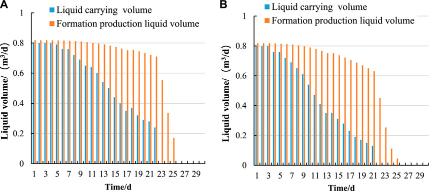
FIGURE 8. Changes in formation produced liquid volume and gas liquid-carrying volume (upslope type (A), downslope type (B)).
For the upturned horizontal well, the early liquid accumulation is located at the root of the horizontal section, and the impact on the formation is relatively small. Therefore, the decline rate of gas production is smaller, and the corresponding changes in formation liquid production and gas carrying capacity are smaller. For the downturned horizontal well, liquid accumulation begins to affect the formation by creating backpressure, reducing the formation productivity, and causing significant decreases in formation liquid production and gas carrying capacity. After 28 days of liquid loading production, the gas production rate of the upturned horizontal well drops to the point where it completely loses the ability to carry liquids, and after 32 days of production, the gas production rate is almost zero, with no formation liquid production. For the downturned inclined horizontal well, the gas well has completely lost the ability to carry liquids after 22 days of production, and both gas and liquid production stopped after 26 days from the formation. Overall, under the same conditions, the impact of liquid accumulation on the upturned horizontal well is relatively small, with longer stable gas production time and greater overall liquid carrying capacity.
(1) Based on the liquid film carrying model, a liquid accumulation prediction model for shale gas wells was established considering the coupling of reservoir supply capacity and wellbore lift capacity, which can accurately predict the changes of liquid accumulation height, gas productivity, and bottomhole pressure of liquid loading gas wells.
(2) The liquid accumulation patterns of upturned sloping and downturned sloping horizontal wells were compared and analyzed. Before the liquid accumulation fills the horizontal section, the liquid accumulation height increases slowly, while after it fills the horizontal section, the liquid accumulation height increases rapidly. Compared to upturned-type horizontal wells, downturned-type horizontal wells are more sensitive to liquid accumulation, and their liquid accumulation height rises more rapidly.
(3) The prediction model is based on the liquid film carrying model and is applicable only to the annular flow pattern of the wellbore. It has certain limitations and cannot be used for other flow patterns.
The original contributions presented in the study are included in the article/supplementary material, further inquiries can be directed to the corresponding author.
JN writing-original draft, conceptualization. LQ software, data curation, resources. BW formal analysis, methodology. WW writing—review and editing. ML resources, investigation. CZ visualization, investigation. All authors contributed to the article and approved the submitted version.
Authors JN, LQ, and BW were employed by CNPC Chuanqing Drilling Engineering Co., Ltd.
The remaining authors declare that the research was conducted in the absence of any commercial or financial relationships that could be construed as a potential conflict of interest.
All claims expressed in this article are solely those of the authors and do not necessarily represent those of their affiliated organizations, or those of the publisher, the editors and the reviewers. Any product that may be evaluated in this article, or claim that may be made by its manufacturer, is not guaranteed or endorsed by the publisher.
Beggs, D. H., and Brill, J. P. (1973). A study of two-phase flow in inclined pipes. J. Petroleum Technol. 05, 607–617. doi:10.2118/4007-pa
Bendiksen, K. H. (1984). An experimental investigation of the motion of long bubbles in inclined tubes. Int. J. Multiph. Flow. 4, 467–483. doi:10.1016/0301-9322(84)90057-0
Du, J., Zhang, H., WangW, , Ma, X., and Zhang, P. (2004). Node analysis method in consideration of discharge fluids in gas well and its application. Nat. Gas. Ind. 1, 43–46. doi:10.3321/j.issn:1000-0976.2004.01.014
Gaol, A. H., and Valko, P. P. (2016). “Modeling wellbore liquid-content in liquid loading gas wells using the concept of characteristic velocity,” in Proceedings of the SPE low perm symposium (Denver, Colorado, USA.
Garcia, A. P., de Sousa, P. C., and Waltrich, P. J. (2016). “A transient coupled wellbore-reservoir model using a dynamic IPR function,” in Proceedings of the SPE annual technical conference and exhibition (Dubai: UAE).
Gou, S. (2006). A simple method to determine flow position in gas well. Well Test. 4, 25–26. doi:10.3969/j.issn.1004-4388.2006.04.009
Greene, W. R. (1983). Analyzing the performance of gas wells. J. Petroleum Technol. 7, 1378–1384. doi:10.2118/10743-pa
Guo, B., Ghalambor, A., and Xu, C. (2005). “A systematic approach to predicting liquid loading in gas wells,” in Proceedings of the SPE production operations symposium (Oklahoma, USA: Oklahoma City), 17–19.
Hagedorn, A. R., and Brown, K. E. (1965). Experimental study of pressure gradients occurring during continuous two-phase flow in small-diameter vertical conduits. J. Petroleum Technol. 04, 475–484. doi:10.2118/940-pa
Haluszczak, L. O., Rose, A. W., and Kump, L. R. (2013). Geochemical evaluation of flowback brine from marcellus gas wells in Pennsylvania, USA. Appl. Geochem 28, 55–61. doi:10.1016/j.apgeochem.2012.10.002
Han, S., Cheng, L., and Ning, Z. (2002). A new method for productivity prediction of fractured horizontal wells in gas reservoirs. J. China Univ. Petroleum 04, 36–39. doi:10.3321/j.issn:1000-5870.2002.04.011
Hao, F., Zhang, G., Cheng, L., He, T., and Wang, L. (2006). Research on productivity equation of liquid carrying gas well. Nat. Gas. Ind. 06, 92–94. doi:10.3321/j.issn:1000-0976.2006.06.029
Harmathy, T. Z. (1960). Velocity of large drops and bubbles in media of infinite or restricted extent. A I Ch. E J. 2, 281–288. doi:10.1002/aic.690060222
Ilobi, M. I., and Ikoku, C. U. (1981). “Minimum gas flow rate for continuous liquid removal in gas wells,” in Proceedings of the 56th SPE annual technical conference and exhibition (San Antonio, Texas, USA.
Lea, J. F., and Nickens, H. V. (2004). Solving gas-well liquid-loading problems. J. Petroleum Technol. 4, 30–36. doi:10.2118/72092-jpt
Li, H., Tian, Y., Wang, Y., Sun, Y., and Jiang, B. (2018). Unsteady-state model coupled with horizontal well and heterogeneous gas reservoir. Special Oil Gas Reservoirs 5, 93–98. doi:10.3969/j.issn.1006-6535.2018.05.018
Li, J., Zhang, C., and Zhao, Y. (2011). Steady-state productivity model of fracturing horizontal wells in gas reservoirs. Neijiang Technol. 07, 21–29. doi:10.3969/j.issn.1006-1436.2011.07.019
Li, L., Zhang, L., Liu, Q., Liu, B., and Duan, Z. (2010). Research on steady-state model of horizontal wellbore and gas reservoir coupling. J. Chongqing Univ. Sci. Technol. 03, 41–44. doi:10.3969/j.issn.1673-1980.2010.03.014
Li, X., and Yong, H. (2001). Discussion on the dynamic relationship curve of transient inflow in gas-water co-production wells. Nat. Gas. Ind. 3, 65–67. doi:10.3321/j.issn:1000-0976.2001.03.020
Liang, Q., Zou, D., Wang, W., and Yu, D. (2015). Diagnosis of liquid loading in water-producing condensate gas wells. Natural Gas Exploration and Development, 01, 57–59. doi:10.3969/j.issn.1673-3177.2015.01.013
Liu, A., Guo, P., Li, Y., Liu, H., Tang, S., Yang, M., et al. (2009). Wellbore zero liquid flow research. Oil Drill. Prod. Technol. 4, 75–78. doi:10.3969/j.issn.1000-7393.2009.04.018
Liu, L., and Zhou, F. (2002). Study on liquid holdup and resistance characteristics of zero net liquid flow two-phase flow. J. Eng. Thermophys. 3, 365–368. doi:10.3321/j.issn:0253-231X.2002.03.030
Liu, T., Guo, X., Wang, Y., Chen, H., Lu, G., and Tong, Y. (2017). Borehole pressure and liquid level prediction of liquid-loading horizontal wells in west Sichuan. Oil Drill. Prod. Technol. 1, 97–102. doi:10.13639/j.odpt.2017.01.019
Liu, J, Xue, Y, Fu, Y, Yao, K., and Liu, J. (2023). Numerical investigation on microwave-thermal recovery of shale gas based on a fully coupled electromagnetic, heat transfer, and multiphase flow model. Energy 263, 126090. doi:10.1016/j.energy.2022.126090
Meng, H., Xu, Y., Chen, D., Zhang, K., Chang, F., and Jiang, D. (2019). Research on calculation model of fluid height in wellbore of gas well. Complex Hydrocarb. Reserv. 1, 81–85. doi:10.16181/j.cnki.fzyqc.2019.01.017
Pagan, E. V., and Waltrich, P. J. (2016). A simplified model to predict transient liquid loading in gas wells. J. Nat. Gas. Sci. Eng. 35, 372–381. doi:10.1016/j.jngse.2016.08.059
Riza, M. F., Hasan, A. R., and Kabir, C. S. (2016). A pragmatic approach to understanding liquid loading in gas wells. SPE Prod. Oper. 03, 185–196. doi:10.2118/170583-pa
Schiferli, W., Belfroid, S., Savenko, S., Veeken, C., and Hu, B. (2010). “Simulating liquid loading in gas wells,” in Proceedings of the 7th north American conference on multiphase Technology (Banff: Canada).
Shen, W., Deng, D., Liu, Q., Gong, J., Chen, X., Yin, Z., et al. (2019b). Characterization and comparison of postnatal rat meniscus stem cells at different developmental stages. J. Chem. Industry 04, 1318–1329. doi:10.1002/sctm.19-0125
Shen, W., Deng, D., Liu, Q., and Gong, J. (2019a). Prediction model of critical gas velocities in gas wells based on annular mist flow theory. CIESC Jorunal 4, 1327–1339. doi:10.11949/j.issn.0438-1157.20180851
Sousa, P. C., Garcia, A. P., and Waltrich, P. J. (2017). “Analytical development of a dynamic IPR for transient two-phase flow in reservoirs,” in Proceedings of the SPE annual technical conference and exhibition (San Antonio, Texas, USA, 9–11.
Stefan, B., Wouter, S., and Veeken, M. (2008). “Predicting onset and dynamic behaviour of liquid loading gas wells,” in Proceedings of the 2008 SPE annual technical conference and exhibition (Denver, Colorado, USA, 21–24.
Sun, F., Han, S., and Chen, L. (2005). Coupling model of seepage flow and wellbore tubular flow in fractured horizontal wells in low-permeability gas reservoirs. J. Southwest Petroleum Inst. 01, 32–36. doi:10.3863/j.issn.1674-5086.2005.01.009
Tang, Y. (2019). Research on shale gas wellbore flow-horizontal well productivity coupling model. Master's thesis. Chengdu, China: Southwest Petroleum University.
Tie, K. (2012). Numerical simulation research on the coupling of horizontal wellbore and gas reservoir flow. Sci. Technol. Eng. 18, 4515–4517. doi:10.3969/j.issn.1671-1815.2012.18.042
Turner, R. G., Hubbard, M. G., and Dukler, A. E. (1969). Analysis and prediction of minimum flow rate for the continuous removal of liquids from gas wells. J. Petroleum Technol. 11, 1475–1482. doi:10.2118/2198-pa
Van Gool, F., and Currie, P. K. (2008). An improved model for the liquid-loading process in gas wells. SPE Prod. Oper. 04, 458–463. doi:10.2118/106699-pa
Vincent, M. C. (2012). The next opportunity to improve hydraulic-fracture stimulation. J. Petroleum Technol. 3, 118–127. doi:10.2118/144702-jpt
We, N., Li, Y., Meng, Y., Li, Y., and Liu, A. (2009). Experimental study on visualization of zero liquid flow in gas wells. Oil Field Equip. 4, 48–51. doi:10.3969/j.issn.1001-3482.2009.04.014
Xiong, Y., Liu, B., Xu, W., Tan, B., and Huang, Y. (2015). Two simple methods to accurately predict liquid loading in low permeability and low production gas wells. Special Oil Gas Reservoirs 2, 93–96. doi:10.3969/j.issn.1006-6535.2015.02.023
Yang, Z., Zhao, C., Liu, X., Li, J., and Huang, C. (2011). Judgment of fluid accumulation and calculation of fluid accumulation depth in gas wells of dalaoba condensate oil and gas field. Nat. Gas. Ind. 9, 62–64. doi:10.3787/j.issn.1000-0976.2011.09.010
You, X., Li, Y., Li, Y., Liu, X., Sun, Y., Wang, L., et al. (2016). Calculation method of fluid accumulation height in downhole choke gas wells in Sulige gas field. Petrochem. Ind. Appl. 03, 85–88. doi:10.3969/j.issn.1673-5285.2016.03.022
Yuan, G., Pereyra, E., Sarica, C., and Sutton, R. P. (2013). “An experimental study on liquid loading of vertical and deviated gas wells,” in Proceedings of the SPE production and operations symposium (Oklahoma, USA: Oklahoma City), 23–26.
Zhang, G., and Chen, J. (2008). Fluid accumulation and drainage period prediction technology for gas wells. J. Oil Gas Technol. 6:328–331.
Zhang, L., Luo, C., Liu, Y., and Zhao, Y. (2019). Research progress in liquid loading prediction of gas wells. Nat. Gas. Ind. 1, 57–63. doi:10.3787/j.issn.1000-0976.2019.01.006
Zhou, C., Dong, D., Wang, Y., Li, X., Huang, J., Wang, S., et al. (2016). Characteristics, challenges and prospects of shale gas in China (2). Pet. Explor Dev. 2, 166–178. doi:10.11698/PED.2016.02.02
Keywords: liquid loading, liquid level, shale gas wells, liquid film model, fluid accumulation prediction
Citation: Nie J, Qiao L, Wang B, Wang W, Li M and Zhou C (2023) Prediction of dynamic liquid level in water-producing shale gas wells based on liquid film model. Front. Earth Sci. 11:1230470. doi: 10.3389/feart.2023.1230470
Received: 29 May 2023; Accepted: 09 August 2023;
Published: 22 August 2023.
Edited by:
Jiexun Li, Western Washington University, United StatesReviewed by:
Jia Liu, Xi’an University of Technology, ChinaCopyright © 2023 Nie, Qiao, Wang, Wang, Li and Zhou. This is an open-access article distributed under the terms of the Creative Commons Attribution License (CC BY). The use, distribution or reproduction in other forums is permitted, provided the original author(s) and the copyright owner(s) are credited and that the original publication in this journal is cited, in accordance with accepted academic practice. No use, distribution or reproduction is permitted which does not comply with these terms.
*Correspondence: Weiyang Wang, d2FuZ3dlaXlhbmdAdXBjLmVkdS5jbg==
Disclaimer: All claims expressed in this article are solely those of the authors and do not necessarily represent those of their affiliated organizations, or those of the publisher, the editors and the reviewers. Any product that may be evaluated in this article or claim that may be made by its manufacturer is not guaranteed or endorsed by the publisher.
Research integrity at Frontiers
Learn more about the work of our research integrity team to safeguard the quality of each article we publish.