An automatic preselection strategy for magnetotelluric single-site data processing based on linearity and polarization direction

The magnetotelluric response function can be severely disturbed by cultural electromagnetic noise. The preselection strategy is one of the effective ways to remove the influence of noise when calculating the response function. This study proposed three new parameters (the amplitude ratio predicted amplitude ratio and linear coherence (PLcoh) between the predicted and observed electric fields and the dispersion degree of the magnetic polarization direction (${DD}_{pol}$)) to detect noisy data, making the preselection strategy automatic. The first two were used to evaluate the linearity of binary linear regression to constrain incoherent noise, while the last was used to evaluate the magnetic polarization direction to constrain coherent noise. Finally, the technique is illustrated by applying it to two field datasets and comparing it with the previous studies. The results showed that these parameters can be used to effectively identify contaminated data, and a reliable response function can be obtained by using these parameters to extract high-quality data when intermittent noise contaminates field data.

1 Introduction

The magnetotelluric (MT) method is an electromagnetic (EM) geophysical method used to infer the subsurface electrical conductivity from the natural geomagnetic and geoelectric fields obtained at the Earth’s surface (Tikhonov, 1950; Cagniard, 1953). There is a linear relationship between the geoelectric and geomagnetic fields in the frequency domain, and it can be expressed as follows (Tikhonov and Berdichevsky, 1966):

$\left(\begin{array}{c}{E}_x\left(\omega \right)\\ E_y\left(\omega \right)\end{array}\right)=\left(\begin{array}{c}{Z}_{xx}\left(\omega \right)Z_{xy}\left(\omega \right)\\ Z_{yx}\left(\omega \right)Z_{yy}\left(\omega \right)\end{array}\right)\left(\begin{array}{c}{H}_x\left(\omega \right)\\ H_y\left(\omega \right)\end{array}\right),(1)$

where E and H are the horizontal electric and magnetic field components at a specific frequency, respectively, $\mathrm{\omega }$ denotes the angular frequency, and Z represents the MT impedance. The subscripts x and y denote two orthogonal directions. The conventional MT impedance estimator first transforms the time-series data into the frequency domain by the windowed Fourier transformation and then performs regression in the frequency domain to calculate the impedance (Jones et al., 1989; Smirnov, 2003; Chave and Jones, 2012). The least-squares (LS) estimator (Sims et al., 1971) is a basic method used for linear regression; it requires the magnetic field to be noise-free, and the residuals between the predicted and observed electric fields are uncorrelated and follow a multivariate normal probability distribution (Chave and Thomson, 1989). However, field data consist of natural sources and local cultural noise (Szarka, 1988; Junge, 1996), these assumptions often fail, and the LS estimator can be severely disturbed by cultural noise.

Methods to remove these disturbances are mainly based on robust statistical algorithms, remote reference processing, multistation analyses or time series modification. The robust statistical methods are based on data-adaptive weighting schemes, which aim to detect and reject outliers from a majority of well-behaved samples (Egbert and Booker, 1986; Chave and Thomson, 2004; 2003; 1989; Jones et al., 1989). These methods require reasonable proportions of normal data to yield reliable results, e.g., data with no more than 50% contamination (Smirnov, 2003). If a noise source is more persistent, it can easily result in a distribution of the majority of the data, which is wrong (Weckmann et al., 2005). The remote reference method requires simultaneously recorded EM fields from at least two sites. Remote reference processing uses cross-power spectra instead of auto-power spectra when performing regression based on the least-squares estimator (Goubau et al., 1978; Gamble et al., 1979). The remote reference method cannot always improve the results, as a successful application requires a horizontal magnetic field at a remote site without correlated noise. It is difficult to find a suitable reference site because cultural noise signals can be widespread and coherent over large areas (Weckmann et al., 2005), and we are faced with single-site robust processing. Moreover, MT researchers have proposed multistation analyses. Larsen et al. (1996) and Oettinger et al. (2001) proposed the signal-noise separation (SNS) method. SNS uses the remote magnetic field to estimate the interstation transform function as the separation tensor; they separated the local magnetic field into signal and noise parts and then calculated the impedance. Egbert (1997) proposed a robust multivariate errors-in-variables estimator (RMEV) to separate field data into signal and noise components using principal component analysis. A more recent application of the method is shown in Smirnov and Egbert (2012). Both the RMEV and SNS methods use a robust approach to their data processing. Those methods may be biased when the majority of the data are contaminated and the noise is coherent between the local and remote sites. In a strong noise environment, the time series modification method is also effective in suppressing the influence of noise (Chen et al., 2022; Li et al., 2022; Li et al., 2023; Li et al., 2018; Zhang et al., 2022; Zhang et al., 2021; Zhou et al., 2022; Wang et al., 2017; Kappler, 2012). These methods identify abnormal waveforms in the time domain and modify the original time series, and they are useful for data contaminated by strong noise with an abnormal waveform.

In a noisy EM environment, as an alternative method, it is practical to use a preselection strategy (Jones and Jödicke, 1984; Travassos and Beamish, 1988; Smirnov, 2003; Chave and Thomson, 2004; Weckmann et al., 2005; Platz and Weckmann, 2019) to reduce the EM noise to a level that the robust statistic method can handle. All of the studies, e.g., Platz and Weckmann (2019), Weckmann et al. (2005), and Garcia and Jones (2002), demonstrated substantially better performance for data-adaptive weighting schemes after prescreening. In theory, if the noise does not contaminate the local site all the time, we can extract high signal-to-noise ratio (SNR) data and obtain a reliable result. The multiple coherence (Jones and Jödicke, 1984; Travassos and Beamish, 1988; Egbert and Livelybrooks, 1996; Bendat and Piersol, 2011) and bivariate coherence (Ritter et al., 1998; Weckmann et al., 2005) are widely used to evaluate the data quality under the assumption that the dataset follows a linear relationship. In this research, we propose a new method, which performs similarly with multiple coherence and is superior to the bivariate coherence, to evaluate the linearity by comparing the similarity between the observed and predicted electric fields. The parameters based on the linearity are effective for detecting incoherent noise, but coherent noise may also have high linearity (Weckmann et al., 2005). In addition, Weckmann et al. (2005) showed the effectiveness of magnetic polarization direction (MPD) in visualizing coherent noise. However, their preselection strategy cannot be performed automatically. Platz and Weckmann (2019) attempted to perform data preselection automatically and used statistical information on the magnetic polarization direction (SMPD) to constrain coherent noise with strong polarization direction. They removed all the data whose polarization directions fall in a bin which is much higher than the threshold. However, the data fall in out of the bin also may correspond to the coherent noise. We proposed a new parameter based on the dispersion degree of the magnetic polarization direction (${DD}_{pol}$) to identify the coherent noise, and the case study shows that it is superior to the criteria based on SMPD. The new parameters are tested on approximately 500 site data from the USArray project (Schultz et al., 2018; Kelbert, 2019) and data collected in China. Finally, two case studies are used to show the effectiveness of the parameters in detecting noisy data and the preselection strategy in improving the quality of the impedance tensor calculation.

The following sections are organized as follows. Section 2 introduces the new parameters proposed to detect noise. Section 3 shows the effectiveness of the parameters to detect noise and compares the new parameters with the previous study.

2 Parameters proposed for the preselection strategy

The method to obtain the spectra of EM fields in different frequencies is similar to the method used in the bounded influence remote reference processing (BIRRP) code (Chave and Thomson, 1989; Chave and Thomson, 2004; 2003). The time series is prewhited and divided into adjacent segments. These segments are cosine tapered before the Fourier transformation. Then, the Fourier coefficients are corrected for the influence of the instrument response. Next, selected frequencies within each segment are extracted to calculate the impedance tensor and uncertainty followed by the robust estimator created by Neukirch and García (2014). At last, the segment length is variable, the previous steps are repeated to calculate the impedance in different frequencies. During data processing, one segment corresponds to one data in the frequency domain. In the following, we refer to one data as one event in the frequency domain. The key to obtaining a reliable impedance from the noisy site is detecting and removing the noise before the impedance estimation. This section introduces the parameters used to detect noisy events from the perspective of linearity and MPD.

2.1 Noise detection based on linearity

From the perspective of whether the data follow the linear relationship in Eq. 1, the field data (E and H) can be subdivided into three parts as follows:

$\mathit{E}=\left\{{\mathit{E}}^{\mathit{M}\mathit{T}},{\mathit{E}}^{\mathit{H}\mathit{L}\mathit{N}},{\mathit{E}}^{\mathit{L}\mathit{L}\mathit{N}}\right\},(2)$

$\mathit{H}=\left\{{\mathit{H}}^{\mathit{M}\mathit{T}},{\mathit{H}}^{\mathit{H}\mathit{L}\mathit{N}},{\mathit{H}}^{\mathit{L}\mathit{L}\mathit{N}}\right\},(3)$

where the superscript HLN denotes the data dominated by noise with high linearity, the superscript LLN denotes the data dominated by noise with low linearity, and the superscript MT denotes the high-quality data with high linearity. Noise with low linearity can be identified from the similarity between the observed electric field and that predicted by the linear relationship. It is similar to the single-input/single-output linear model to evaluate the linearity, as shown in Figure 1. The difference between the data with high linearity and low linearity is that most of the predicted and observed values of the output are similar.

FIGURE 1

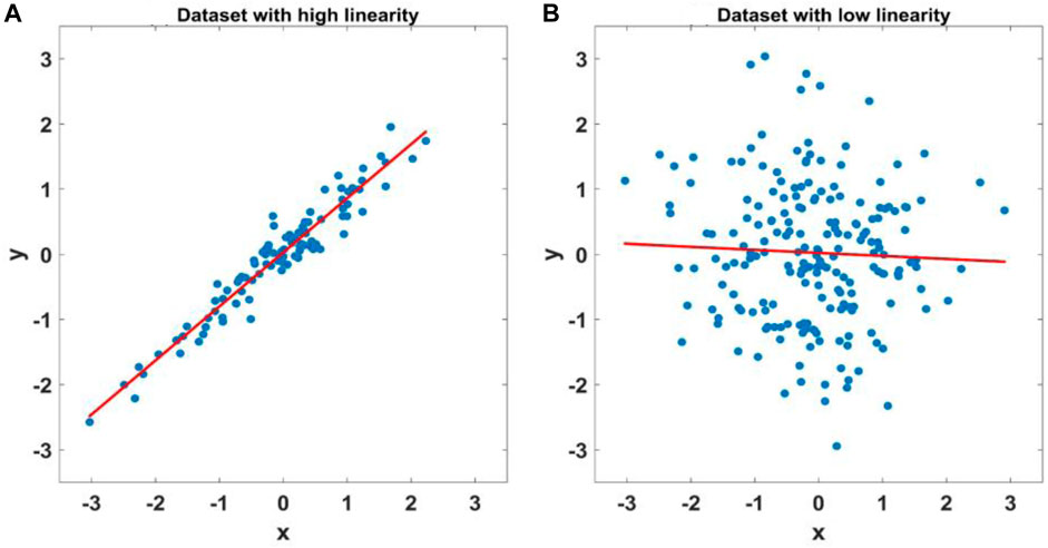
FIGURE 1. Single-input/single-output linear model y=a*x+b. x is the input, and y is the output. The blue points denote the observed data, and the red line is the model calculated by regression. The difference between the data with high linearity and low linearity is that most of the predicted values (a*x+b) calculated by the model and the output (y) are similar, as shown in (A) and (B).

Assuming the data are highly linear related, the observed electric field (E) should be similar to the predicted electric field (${\mathit{E}}_{\mathit{p}}$), where ${\mathit{E}}_{\mathit{p}}$ =ZH and Z are obtained by the least-squares estimator. We can identify noisy data with low linearity by comparing the measured electric field (E) and the predicted electric field (${\mathit{E}}_{\mathit{p}}$). The complex number has two properties: the amplitude and phase. In this study, we use the linear coherence defined by the phase difference between the predicted and observed electric fields to confirm the phase similarity and use the amplitude ratio between the predicted and observed electric fields to confirm the amplitude similarity.

The linear coherence (Lcoh) between two spectra $A_i$ and $B_i$ is defined by the cosine of the phase difference (PD) as follows:

$\cos \left({\theta }_i\right)=\mathrm{R}\mathrm{e}\left(e^{j\left({\phi }_{A_i}-{\phi }_{B_i}\right)}\right)=\mathrm{R}\mathrm{e}\left(\frac{A_i{\overline{B}}_i}{\left.{\left|A\right.}_i\Vert B_i\right|}\right),(4)$

where $A_i$ and $B_i$ denote the spectrum calculated from the i^th segment, ${\overline{B}}_i$ represents a conjugate of $B_i$, and ${\theta }_i$ denotes the angle of the phase difference (PD) between $A_i$ and $B_i$. According to Euler’s formula, Lcoh equals the real part of $e^{\left.{j(\phi }_{A_i}-{\phi }_{B_i}\right)}$. Re denotes the real part of the complex number. The value of Lcoh lies in the range of (−1,1). When the PD is close to 0 $°$, the Lcoh is high and close to 1. In this study, the predicted linear coherence (P $Lcoh$) between the measured electric field (E) and the predicted electric field (${\mathit{E}}_{\mathit{p}}$) is calculated as follows:

$PLcoh=\mathrm{R}\mathrm{e}\left(\frac{Y_{p_i}{\overline{Y}}_i}{\left|Y_{p_i}\Vert Y_i\right|}\right),(5)$

where $Y_{p_i}$ and $Y_i$ are the predicted and measured electric fields corresponding to the i^th segment, and Y is associated with either $E_x$ or $E_y$. The predicted electric field and the observed electric field should be similar when the linearity is high, and PLcoh should be close to 1.

The high predicted linear coherence can ensure the phase similarity. We also use the predicted amplitude ratio (PAR) to ensure the amplitude similarity, and it is defined as follows:

$PAR=\{\begin{array}{c}\frac{\left|Y_{p_i}\right|}{\left|Y_i\right|},\left|Y_{p_i}\right|<\left|Y_i\right|,or\\ \frac{\left|Y_i\right|}{\left|Y_{p_i}\right|},\left|Y_i\right|<\left|Y_{p_i}\right|.\end{array}(6)$

The PAR ranges from 0 to 1; the higher PAR is, the higher the similarity between the two spectra in terms of the amplitude.

There is a problem that the energy of the signal and noise changes with time, and the linearity may change. Suppose we perform regression with all the available data; the linearity may be low in the presence of a large amount of noise and provide misleading information. It is similar to the single-input/single-output linear model, as shown in Figure 2. There are six datasets, and only dataset 1 has high linearity. When we perform regression with all the available data, the linearity is low, and we cannot extract data with high linearity. To solve this problem, we subdivide the data into small groups and calculate the PAR and PLcoh values separately. We rename the predicted linear coherence and amplitude ratio as ${PLcoh}_{sz}$ and ${PAR}_{sz}$, where the subscript SZ means we calculate the predicted electric field (${\mathit{E}}_{\mathit{p}}$ =ZH) by the impedance (Z) obtained by the subdivided data. In this research, the field data are subdivided into small groups with 20 samples when evaluating the linearity. It is necessary to divide the data into groups when evaluating linearity (see Supplementary Figures S2, S3).

FIGURE 2

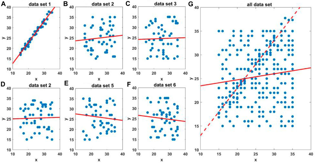
FIGURE 2. Single-input/single-output linear model y=a*x+b. (A–F) show the regression results for six datasets separately; each dataset has 50 points, and only dataset 1 has high linearity. The blue points denote the observed data, and the red line is the model calculated by regression. (G) shows the regression results for all the available data, including 300 points. The red solid line denotes the model calculated by all the available data, and the dashed line denotes the model calculated by dataset 1.

2.2 Noise detection based on the magnetic polarization directions

Fowler et al. (1967) proposed the polarization direction, and Weckmann et al. (2005) showed the effectiveness of MPD in detecting coherent noise. The MPD (${\alpha }_{H_i}$) at a specific frequency is defined as follows:

${\alpha }_{H_i}={\mathit{tan}}^{-1}\frac{2Re\left(H_{x_i}{\overline{H}}_{y_i}\right)}{{\left|H_{x_i}\right|}^2-{\left|H_{y_i}\right|}^2}={\mathit{tan}}^{-1}\frac{2\frac{\left|H_{y_i}\right|}{\left|H_{x_i}\right|}·\mathit{cos}\left({\theta }_i\right)}{1-{\left(\frac{\left|H_{y_i}\right|}{\left|H_{x_i}\right|}\right)}^2},(7)$

where i (=1,2, … , N) is the number index of the event, $H_{x_i}$ and $H_{y_i}$ are the spectra of the magnetic field calculated from the i^th segment, and ${\theta }_i$ denotes the PD between $H_{x_i}$ and $H_{y_i}$. The polarization direction is related to the PD and amplitude ratio (AR) between the two orthogonal fields. Various sources generate natural magnetic signals that vary in incident directions and energy, and the PD and AR between the two orthogonal fields vary with time; thus, the magnetic field has no preferred polarization direction (Weckmann et al., 2005). In contrast, the local EM noise source usually has a constant location; the incident direction and energy have similar properties that change with time. Suppose there is a preferred polarization direction for the magnetic field; we can consider that the coherent noise contaminates the data. On the other hand, when incoherent noise contaminates the field data, the magnetic field has no preferred polarization direction. Therefore, the polarization direction for the magnetic field can only detect coherent noise.

To quantify the dispersion degree of MPD, the dispersion degree of the polarization directions (${DD}_{pol}$) is proposed as follows:

${DD}_{pol}=\frac{N_{in}}{N},(8)$

where $N_{in}$ denotes the number of samples falling in the range of ($m_i$ + 30 $°$, $m_i$-30 $°$). $m_i$ is the median for each ${\alpha }_{H_i}$ with its surrounding 2k samples (k is set to 20 in this study), and it is calculated as follows:

$m_i=\mathrm{m}\mathrm{e}\mathrm{d}\mathrm{i}\mathrm{a}\mathrm{n}\left({\alpha }_{H_{i-k}},{\alpha }_{H_{i-k-1}},\dots ,{\alpha }_{H_i},\dots ,{\alpha }_{H_{i+k-1}},{\alpha }_{H_{i+k}}\right).(9)$

When the polarization direction has a preferred direction, $m_i$ approximately equal to the preferred direction. $m_i$ is calculated by the surrounding 2k samples, and there are two sides; we hope half of the data is beyond a specific range, which means the threshold is set as 0.5; therefore, the expected value of ${DD}_{pol}$ should be smaller than 0.5, and 1/3 is chosen in this research, which means the range is 60 $°$ (180 $°\times$ 1/3), and the specific range is set as ($m_i$ + 30 $°$, $m_i$-30 $°$). If the polarization directions vary randomly from −90 $°$ to 90 $°$, ${DD}_{pol}$ should be close to 1/3, and ${DD}_{pol}$ increases when there is a preferred direction. ${DD}_{pol}$ can be used to automatically detect coherent noise with a strong polarization direction.

3 Case studies for the preselection strategy

Usually, data dominated by incoherent noise do not have a stable relationship; therefore, the linearity should be low. We can identify the incoherent noise using the parameters ${PLcoh}_{sz}$ and ${PAR}_{sz}$. According to the linearity and MPD of the data, the data quality can be classified into three types, as shown in Table 1. Combining the linearity and the MPD, we can constrain both coherent and incoherent noise simultaneously.

TABLE 1

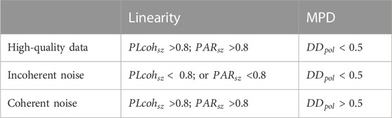
TABLE 1. Classification of the data quality based on the linearity and MPD.

The preselection strategy based on linearity and the MPD is tested on approximately 500 site data from the USArray project (Schultz et al., 2018; Kelbert, 2019) and data collected in China. It can improve the quality of the impedance tensor when intermittent noise contaminates the field data. Two typical field datasets are chosen to demonstrate the effectiveness of those parameters to identify noisy events. The location map is shown in Figure 3. The first data are contaminated by incoherent noise, which contains a geomagnetic storm, the energy from the natural EM signal increases significantly, and high signal-to-noise ratio (SNR) data appear during the storm. The second dataset is contaminated by coherent noise and incoherent noise simultaneously, the noise decreases during the local nighttime, and high SNR data appear.

FIGURE 3

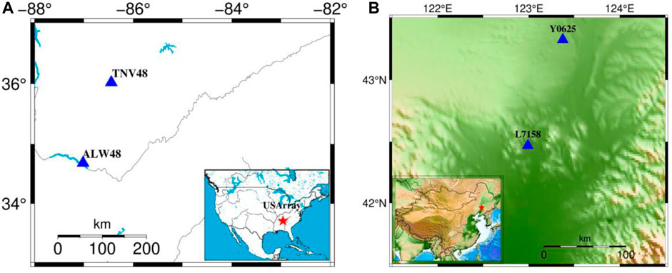
FIGURE 3. Location map of the field data. (A) shows the location of the first field data; the blue triangles denote the observation site. TNV48 is used as the locale site, and ALW48 is set as the remote reference site. The lower right corner in (A) shows the survey location of the USArray, and the red star denotes the location of site TNV48. (B) shows the location map of the second field data observed in China. Y0625 is the remote reference site, and L7-158 is the local site. The lower left corner in (B) shows the survey area in China, and the red star denotes the local site.

3.1 Case study 1: Data contaminated by intermittent incoherent noise

The first case study used the data observed at TVN48 from the USArray project. The time-series data can be downloaded from the Incorporated Research Institutions for Seismology (IRIS) website. The data sampling period is 1 s, and the used times-series data are observed from July 19 to 24 July 2015. First, we examine the variation in the parameters at different frequencies. Figure 4 shows the parameter variation in the period of 13.1 s. Figures 4A, B show the variation in ${PLcoh}_{sz}$ and ${PAR}_{sz}$ associated with $E_x$-component, respectively. The events in which both ${PLcoh}_{sz}$ and ${PAR}_{sz}$ are larger than 0.8 are shown in red, and the other is shown in blue. Red denotes an event with high linearity, and blue denotes an event with low linearity. Figure 4C shows that the MPD is scattered for all the events. Figure 4D shows the variation in the hat matrix’s diagonal element. The hat matrix is an N by N matrix (N denotes the number of events) defined as follows (Chave and Thomson, 2004; 2003):

${\mathit{H}}_{hat}=\mathit{H}{\left({\mathit{H}}^{†}\mathit{H}\right)}^{-1}{\mathit{H}}^{†},(10)$

where H represents N by two matrices of the horizontal magnetic field (${\mathit{H}}_x,{\mathit{H}}_y$) at a specific frequency. The superscript $†$ denotes the complex conjugate transpose. The expected value of the hat matrix’s diagonal element is 2/N. The variation in the diagonal elements of the hat matrix has the same trend as the magnetic field amplitude (Chen et al., 2022; Li et al., 2022; Li et al., 2023; Li et al., 2018; Zhang et al., 2022; Zhang et al., 2021). Therefore, we can use the hat matrix to visualize the energy variation in the magnetic field. Figure 4D shows that the red events have high energy. This is caused by the geomagnetic storm (see Supplementary Figure S1). Since the natural EM signal is relatively low in the dead band (0.1–10 s), local noise can easily influence it during non-storm periods. When there is a geomagnetic storm, the natural EM signal strength increases, and high SNR events appear. In conclusion, the blue events are dominated by incoherent noise in the period of 13.1 s, and ${PLcoh}_{sz}$ and ${PAR}_{sz}$ can identify incoherent noise. Figure 5 shows the parameter variation in the period of 105.4 s. Most of the events have high linearity, and the MPD is scattered for all the events. This indicates that only a small part of the events are contaminated by incoherent noise. After analyzing the variation in the parameters in different periods, we found that most of the events are dominated by incoherent noise between 5 and 20 s.

FIGURE 4

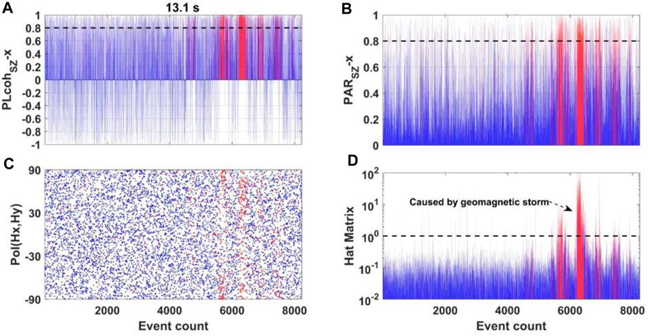
FIGURE 4. Parameters variation at TVN48 in the period of 13.1 s. The horizontal axis denotes the event count. Panels (A, B) show the variation in ${PLcoh}_{sz}$ and ${PAR}_{sz}$ associated with $E_x$-component, respectively. The red color denotes the events in which both ${PLcoh}_{sz}$ and ${PAR}_{sz}$ are higher than 0.8, and the other events are shown in blue. (C) shows the variation in the MPD. (D) shows the variation in the hat matrix’s diagonal element, and the hat matrix’s diagonal element is normalized by the expected value.

FIGURE 5

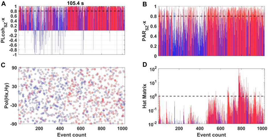
FIGURE 5. Parameters variation at TVN48 in the period of 105.4 s. (A, B) show the variation in ${PLcoh}_{sz}$ and ${PAR}_{sz}$ associated with $E_x$-component, respectively. The red color denotes the events with high linearity, and the other events are shown in blue. (C) shows the variation in MPD. (D) shows the variation in the hat matrix’s diagonal element.

Then, we compare the MT sounding curves calculated by the different methods, as shown in Figure 6. All of those responses are estimated by M-estimator (Egbert and Booker, 1986; Neukirch and García, 2014; Maronna et al., 2019). The result using the data preselection strategy with ${PLcoh}_{sz}$ and ${PAR}_{sz}$ coincides with the remote reference result, and they are regarded as the true model. It shows that a reliable result can be obtained even if we do not use the remote site data by the preselection method. On the other hand, the apparent resistivity of the robust results is downbiased between 6 and 20 s. According to the analysis of Figure 4, more than half of the events are contaminated by incoherent noise. The underestimation of the apparent resistivity was probably attributed to the auto-power spectra of the noise in the denominator of the response function, which is a well-known limitation of the single-site data processing (Sims et al., 1971; Simpson and Bahr, 2005).

FIGURE 6

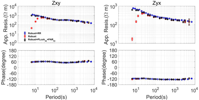
FIGURE 6. MT sounding curves calculated by the different methods using the data observed at site TNV48. The upper figures show the apparent resistivity, and the lower figures show the impedance phase. All the responses are estimated by a M-estimator. The blue curves denote the remote reference results. The red curves denote the single-site robust result. The black curves are calculated by the preselection strategy using ${PLcoh}_{sz}$ and ${PAR}_{sz}$, and the threshold is set to 0.8 for both ${PLcoh}_{sz}$ and ${PAR}_{sz}$. The apparent resistivity of the robust results is downbiased compared with other results between 5 and 20 s.

3.2 Comparison of the parameters used to evaluate the linearity

This subsection compares the performance of the related parameters used to evaluate linearity, e.g., multiple coherence (Travassos and Beamish, 1988; Egbert and Livelybrooks, 1996; Bendat and Piersol, 2011) and bivariate coherence (Ritter et al., 1998; Weckmann et al., 2005). All of those parameters can be indicators of the data quality under the assumption that the dataset follows a linear relationship.

Multiple coherence is defined as the ratio of the ideal output spectrum due to the measured inputs in the absence of noise to the total output spectrum, which includes the noise (Bendat and Piersol, 2011). In equation form, the multiple coherence associated with $E_x$ is calculated as follows:

$r_m^2=1-\frac{E_{{err}_{x_i}}{\overline{E}}_{{err}_{x_i}}}{E_{x_i}{\overline{E}}_{x_i}},(11)$

where $E_{{err}_{x_i}}=E_{p_{x_i}}-E_{x_i},E_{p_{x_i}}and{E}_{x_i}$ denote the predicted and observed electric field calculated by the i^th segment. The bar denotes the conjugate of a complex number. Because the error between the predicted and observed electric field may be larger than the observed electric field. The right part of Eq. 11 may be a negative value. We take the square root of the absolute value of $1-\frac{E_{{err}_{x_i}}{\overline{E}}_{{err}_{x_i}}}{E_{x_i}{\overline{E}}_{x_i}}$ as the multiple coherence ($r_m$), and regard the event, which $r_m$ larger than 0.8 and smaller than 1, are in high linearity. The red events in Figure 7C show the event in high linearity based on the multiple coherence.

FIGURE 7

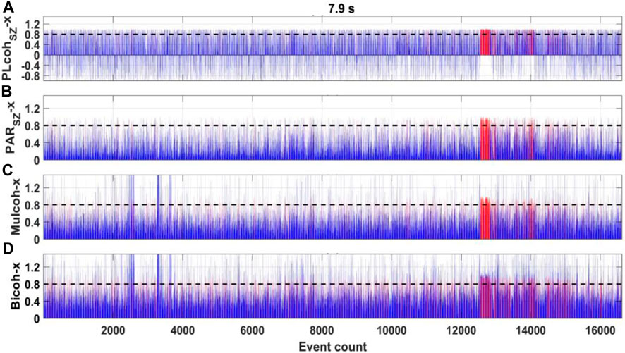
FIGURE 7. Parameters variation at TVN48 in the period of 7.9 s. The red color denotes the events in high linearity based on different parameters, and the other events are shown in blue. All the parameters are determined from the bivariate equations whose dependent variable is the $E_x$-component. (A, B) show the variation in ${PLcoh}_{sz}$ and ${PAR}_{sz}$. The high linearity events are in which both ${PLcoh}_{sz}$ and ${PAR}_{sz}$ are higher than 0.8. (C) shows the variation in multiple coherence. The high linearity events are in which the multiple coherence is higher than 0.8 and smaller than 1. (D) shows the variation in bivariate coherence. The high linearity events are in which the bivariate coherence is higher than 0.8 and smaller than 1.

Bivariate coherence is defined as a function of the amplitude ratio and phase difference between the predicted and the observed electric field. In equation form, bivariate coherence associated with $E_x$ is calculated as follows (Weckmann et al., 2005):

$r_b^2=\frac{Z_{xx}*H_{x_i}{\overline{E}}_{x_i}+Z_{xy}*H_{y_i}{\overline{E}}_{x_i}}{E_{x_i}{\overline{E}}_{x_i}}=\frac{{E_{p_{x_i}}\overline{E}}_{x_i}}{E_{x_i}{\overline{E}}_{x_i}}=\frac{\left|E_{p_{x_i}}\right|}{\left|E_{x_i}\right|}·\mathit{cos}\left({\theta }_i\right),(12)$

where $E_{x_i}$, $H_{x_i}$ and $H_{y_i}$ represent the EM field corresponding to the i^th segment. ${\theta }_i$ is the phase difference between $E_{p_{x_i}}and{E}_{x_i}$. Because the predicted electric field may be larger than the observed electric field, and bivariate coherence may be larger than 1. We regard the event, which $r_b$ larger than 0.8 and smaller than 1, are in high linearity. The red events in Figure 7D show the data in high linearity based on the bivariate coherence.

The comparison of the parameters used to evaluate the linearity is shown in Figure 7. First, the events are divided into groups that contain N samples, e.g., 20 samples. We calculate the predicted electric field for each group, separately. If the data quality is high, all of the parameters should be close to one under the assumption that the data follow a linear relationship. All of the parameters can identify the high-quality data corresponding to the magnetic storm. However, the parameters (${PLcoh}_{sz}$ and ${PAR}_{sz}$) proposed in the research and multiple coherence perform better than bivariate coherence. Some parts of the high-quality events, which $r_b$ larger but close to 1 are regarded as in low linearity based on the bivariate coherence. The MT sounding curves calculated by the different preselection strategies are shown in Figure 8. All of the preselection strategies can reduce the influence of noise compared with the robust result in Figure 6. While the apparent resistivity in Figure 8B around the period of 7.9 s is downbiased compared with other results in Figures 8A, C. It may be caused by some parts of the high-quality events being removed when using the bivariate coherence to prescreen data.

FIGURE 8

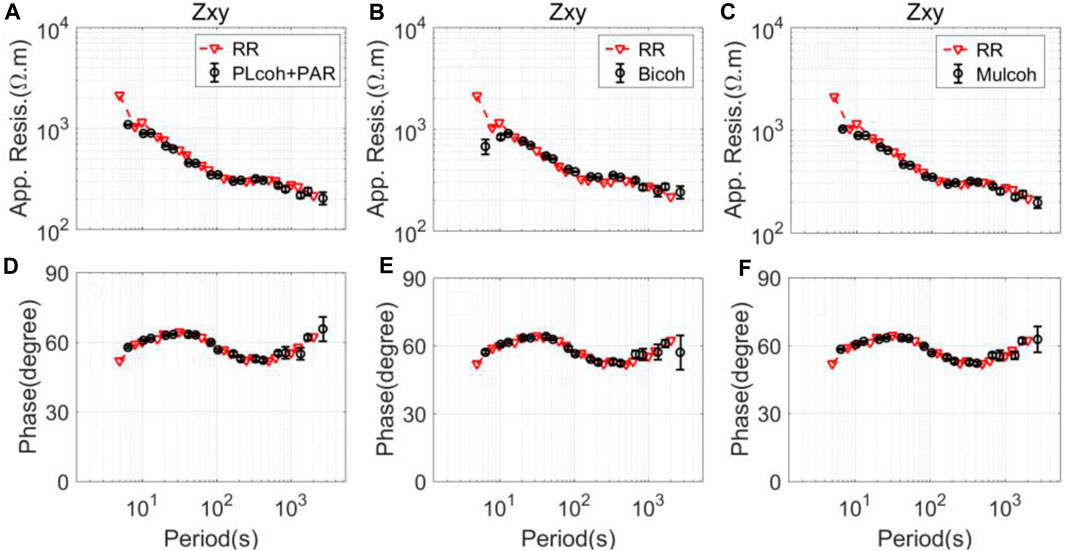
FIGURE 8. MT sounding curves calculated by the different preselection strategies corresponding to $Z_{xy}$ component using the data observed at site TNV48. The upper figures show the apparent resistivity, and the lower figures show the impedance phase. The red curves denote the remote reference results. The black curves denote the result calculated by the different preselection strategies. (A, D) are calculated by the preselection strategy using ${PLcoh}_{sz}$ and ${PAR}_{sz}$. (B, E) are calculated by the preselection strategy using bivariate coherence. (C, F) are calculated by the preselection strategy using multiple coherence. The apparent resistivity in (B) at 7.9 s is downbiased compared with other results in (A, C).

3.2 Case study 2: Data contaminated by intermittent coherent Noise and incoherent noise

The second case study uses data observed in northeastern China on 26 June 2020. Phoenix Geophysics Instruments were used to collect the MT time-series data. These data are provided by the Institute of Geophysical and Geochemical Exploration, China Geological Survey. Time-series data from 3:00 to 22:00 UTC were used in this case study. The sampling rate is 15 Hz. The observation area is in the GMT+8 time zone, and the local midnight time is approximately 16:00.

First, we examine the variation in the parameters at different frequencies. Figure 9 shows the variation in the period of 6.7 s. Red denotes events with high linearity, and blue denotes events with low linearity. The previous 2,500 events in the daytime have a preferred polarization direction of approximately −30 $°$, as shown in Figure 9C, and the polarization direction becomes scattered at nighttime (the events are approximately 2,500 to 4,000). This indicates that the daytime event is dominated by coherent noise, and most of the events have high linearity; in contrast, the event at nighttime is relatively quiet. Figure 10 shows the variation in the period of 33.4 s. The previous 300 events in the daytime have low linearity, and the polarization direction is scattered. In contrast, the events during the nighttime between 300 and 500 have a high linearity, and the polarization direction is scattered. This indicates that the daytime event is dominated by incoherent noise and that the nighttime events are relatively quiet. After analyzing the parameter variation at different frequencies, we find that most of the events are dominated by coherent noise between 2 and 20 s and dominated by incoherent noise between 20 and 100 s. The field data are contaminated by coherent and incoherent noise simultaneously.

FIGURE 9

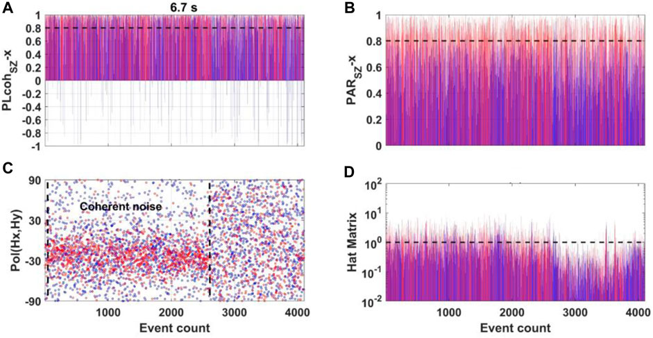
FIGURE 9. Parameters variation at L7-158 in the period of 6.7 s. (A, B) show the variation in ${PLcoh}_{sz}$ and ${PAR}_{sz}$ associated with $E_x$-component, respectively. The red color denotes the events with high linearity, and the other events are shown in blue. (C) shows the variation in the MPD. (D) shows the variation in the hat matrix’s diagonal element.

FIGURE 10

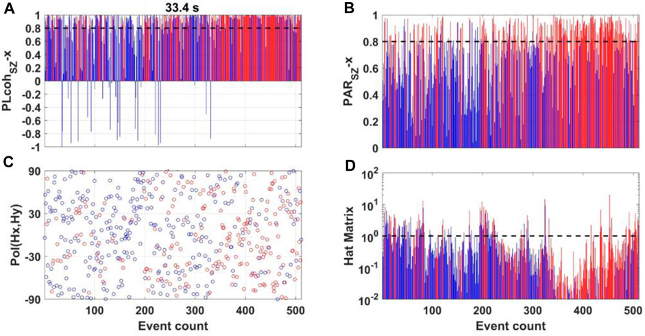
FIGURE 10. Parameters variation at L7-158 in the period of 33.4 s. (A, B) show the variation in ${PLcoh}_{sz}$ and ${PAR}_{sz}$ associated with $E_x$-component, respectively. The red color denotes the events with high linearity, and the other events are shown in blue. (C) shows the variation in the MPD. (D) shows the variation in the hat matrix’s diagonal element.

Then, we compare the MT sounding curves calculated by the different methods. First, we compare the result calculated by the SSMT-2000 and the results with and without the preselection strategy based on linearity, as shown in Figure 11. SSMT-2000 is one of the standard Phoenix software sets. After comparing all the results, we think all the impedance results are biased between 2 and 20 s, and there is a rapid rise and fall in the apparent resistivities. The SSMT-2000 result coincides with the preselection strategy result between 20 and 100 s and changes smoothly. The single-site robust result is improved between 20 and 100 s after using the preselection strategy with ${PLcoh}_{sz}$ and ${PAR}_{sz}$. According to the data quality analysis in different periods, most of the events are contaminated by incoherent noise between 20 and 100 s, and ${PLcoh}_{sz}$ and ${PAR}_{sz}$ are effective in removing incoherent noise. Most of the events are contaminated by coherent noise, which is highly linear, between 2 and 20 s. We also try to use the remote reference method to improve the result but fail (see Supplementary Figure S5), and it needs a different strategy to suppress the noise.

FIGURE 11

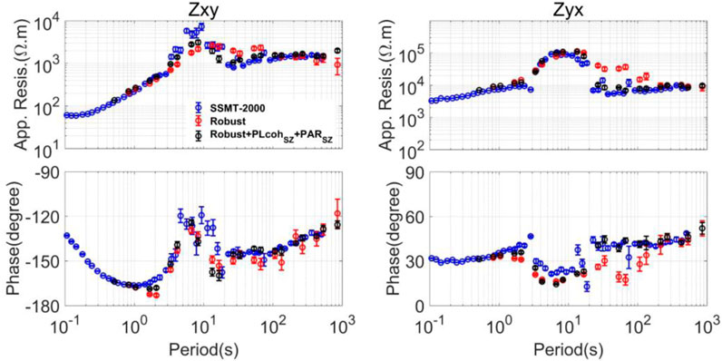
FIGURE 11. MT sounding curves calculated by the different methods using the data observed at site L7-158. SSMT-2000 is used to calculate the blue curves. SSMT-2000 is one of the standard Phoenix software sets. The robust single-site processing approach is used to calculate the red curves. The preselection strategy using ${PLcoh}_{sz}$ and ${PAR}_{sz}$ is used to calculate the black curves.

Next, we try to use the information on MPD to constrain the coherent noise. Figure 12 shows the variation in the MPD and the corresponding variation in ${DD}_{pol}$ in the periods of 6.7 and 33.4 s. The expected value of ${DD}_{pol}$ is 1/3, and ${DD}_{pol}$ increases when the polarization direction has a preferred direction. It shows that ${DD}_{pol}$ is effective in differentiating the events with and without a preferred polarization direction.

FIGURE 12

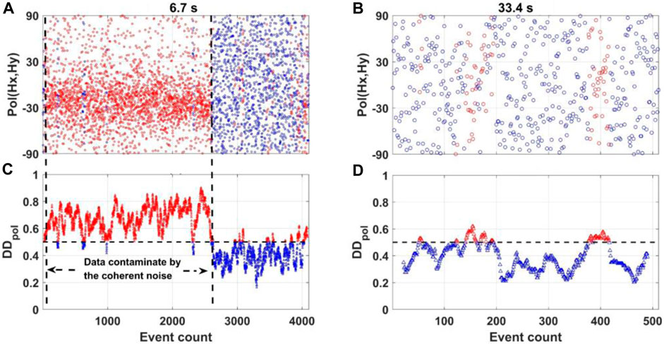
FIGURE 12. Variation in the polarization direction and the corresponding variation in ${DD}_{pol}$ at 6.7 and 33.4 s. (A, B) show the variation in the polarization direction, and (C, D) show the corresponding dispersion degree. The horizontal axis denotes the event count. The red color denotes the events whose dispersion degrees are higher than 0.5, and the other events are shown in blue.

We also compare the criteria proposed by Platz and Weckmann (2019) which is based on the statistical information on magnetic polarization direction (SMPD). They subdivided the polarization direction into 180 bins with a bin width of 1 $°$. In general, the polarization direction is randomly distributed in each bin. Therefore, the expected value $\left(\frac{Numberofevents}{180}\right)$ is the same for each bin. They removed all the events whose polarization directions fall into bins that are much higher than the expected value. Figure 13 shows the statistical analyses of the polarization direction; the threshold k (k = 1.5σ) is used to detect abnormal values, where σ is the standard deviation (Chave and Thomson, 2003). The corresponding abnormal events are drawn in red. According to the criteria based on SMPD, the quiet event may be removed at nighttime (the event from 2,500 to 4,000) and many of the events in the daytime remain.

FIGURE 13

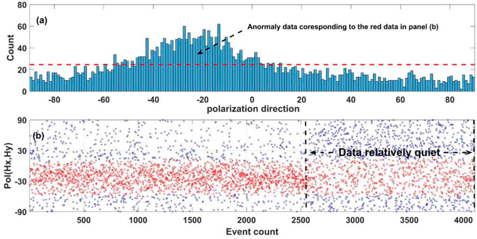
FIGURE 13. Histogram of the MPD and the corresponding variation in the MPD at site L7-158 in the period of 6.7 s. (A) shows the histogram of the MPD; the horizontal axis denotes the bins of the MPD, the vertical axis denotes the number falling in the corresponding bin, and the red dashed line denotes the threshold. (B) shows the variation in the MPD. The horizontal axis denotes the event count. The red color denotes the events that fall into a bin with a higher than expected value, and the other events are shown in blue. The quiet event may be removed at nighttime (the event from 2,500 to 4,000) and many of the events in the daytime remain based on the criteria of SMPD.

At last, we compare the MT sounding curves calculated by the different preselection strategies based on the information on MPD, as shown in Figure 14. The robust estimator combining ${PLcoh}_{sz}$, ${PAR}_{sz}$ for the preselection strategy is used to calculate the blue curve, which prescreens the data only based on the linearity. The robust estimator combining ${PLcoh}_{sz}$, ${PAR}_{sz}$ and SMPD for the preselection strategy is used to calculate the red curve. The criteria proposed by Platz and Weckmann (2019) do not improve the result, the rapid rise and rapid fall between 2 and 20 s remain. The robust estimator combining ${PLcoh}_{sz}$, ${PAR}_{sz}$ and ${DD}_{pol}$ for the preselection strategy is used to calculate the black curve, and the threshold for ${DD}_{pol}$ is set to 0.5. The rapid rise and rapid fall between 2 and 20 s are removed. Comparing the two criteria between ${DD}_{pol}$ and SMPD, most of the events in the daytime are removed based on the ${DD}_{pol}$, while many events in the daytime remain based on the SMPD, and those events in the daytime may also correspond to the coherent noise and dominate the regression, making the preselection strategy fail. This shows the superiority of ${DD}_{pol}$ for detecting coherent noise with a strong magnetic polarization direction.

FIGURE 14

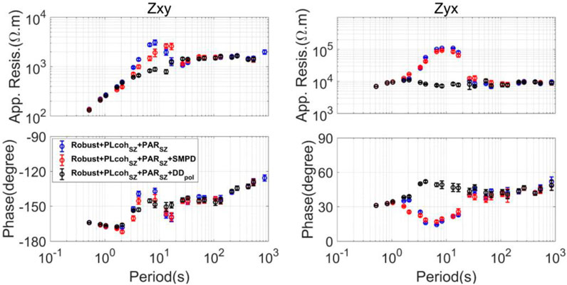
FIGURE 14. MT sounding curves calculated by the different preselection strategies using the data observed at site L7-158. The robust estimator combining ${PLcoh}_{sz}$, and ${PAR}_{sz}$ for the preselection strategy is used to calculate the blue curves. The robust estimator combining ${PLcoh}_{sz}$, ${PAR}_{sz}$ and SMPD for the preselection strategy is used to calculate the red curves. The robust estimator combining ${PLcoh}_{sz}$, ${PAR}_{sz}$ and ${DD}_{pol}$ for the preselection strategy is used to calculate the black curves.

4 Conclusion

Robust single-site data processing may work well unless a large fraction of the data is quiet. On the other hand, the remote reference method may also fail to obtain a reliable result when the noise is correlated between local and remote sites. In a noisy EM environment, it is practical to use a preselection strategy to extract high signal-to-noise ratio (SNR) data, and a reliable response function can be obtained if the noise does not contaminate the local site all the time.

We proposed three new parameters for the preselection strategy from the perspectives of linearity and magnetic polarization, making the preselection process automatic. The predicted linear coherence (${\mathit{P}\mathit{L}\mathit{c}\mathit{o}\mathit{h}}_{\mathit{s}\mathit{z}}$) and amplitude ratio (${\mathit{P}\mathit{A}\mathit{R}}_{\mathit{s}\mathit{z}}$) are combined to evaluate the linearity. We compared the performance with related parameters, e.g., multiple coherence and bivariate coherence. It shows that new parameters proposed in this research (${\mathit{P}\mathit{L}\mathit{c}\mathit{o}\mathit{h}}_{\mathit{s}\mathit{z}}$ and ${\mathit{P}\mathit{A}\mathit{R}}_{\mathit{s}\mathit{z}}$) perform similarly with multiple coherence and better than the bivariate coherence. Linearity can be a general criterion for detecting noisy data with low linearity, which corresponds to incoherent noise. However, coherent noise may also have high linearity (see Supplementary Figure S4). The dispersion degree of the magnetic polarization direction (${\mathit{D}\mathit{D}}_{\mathit{p}\mathit{o}\mathit{l}}$) is proposed to detect coherent noise with a preferred polarization direction, which performs better than the criteria proposed by Platz and Weckmann (2019). It can quantify the polarization change over time. Suppose noise contaminates the local site intermittently; using those parameters may improve the quality of the response function.

Data availability statement

The time-series data from the USArray project are available from IRIS (http://ds.iris.edu/gmap/#network=_US-MT&planet=earth).

Author contributions

HaC processed the time-series data, created the results, and wrote the paper. HaC contributed approximately 50%. ZR, LZ, and HuC reviewed the paper and contributed approximately 30%; GW provided the MT field data and processed the time-series data with SSMT-2000 software. GW contributed approximately 20% to this work.

Funding

This research is financially supported by the National Natural Science Foundation of China (grants 41774086, 41930430), the Major Research plan of the National Natural Science Foundation of China (grant 92262303), and the Key Research Program of the Institute of Geology and Geophysics, Chinese Academy of Sciences (IGGCAS-201901).

Acknowledgments

We are grateful to the Institute of Geophysical and Geochemical Exploration, China Geological Survey, and USArray team members for providing the time-series data used in this study. The valuable comments and suggestions by three reviewers have greatly improved the manuscript. Finally, we thank Ruan Shuai and Hao Zhou for making meaningful comments on the paper’s content.

Conflict of interest

The authors declare that the research was conducted in the absence of any commercial or financial relationships that could be construed as a potential conflict of interest.

The reviewer XZ declared a shared affiliation with the authors HC, ZR to the handling editor at time of review,

Publisher’s note

All claims expressed in this article are solely those of the authors and do not necessarily represent those of their affiliated organizations, or those of the publisher, the editors and the reviewers. Any product that may be evaluated in this article, or claim that may be made by its manufacturer, is not guaranteed or endorsed by the publisher.

Supplementary material

The Supplementary Material for this article can be found online at: https://www.frontiersin.org/articles/10.3389/feart.2023.1230071/full#supplementary-material

References

Bendat, J. S., and Piersol, A. G. (2011). Random data: Analysis and measurement procedures. Hoboken, NJ, United States: John Wiley & Sons.

Google Scholar

Cagniard, L. (1953). Basic theory of the magneto-telluric method of geophysical prospecting. Geophysics 18, 605–635. doi:10.1190/1.1437915

CrossRef Full Text | Google Scholar

Chave, A. D., and Jones, A. G. (2012). The magnetotelluric method: Theory and practice. Cambridge, United Kingdom: Cambridge University Press.

Google Scholar

Chave, A. D., and Thomson, D. J. (2003). A bounded influence regression estimator based on the statistics of the hat matrix. J. R. Stat. Soc. Ser. C Appl. Stat. 52, 307–322. doi:10.1111/1467-9876.00406

CrossRef Full Text | Google Scholar

Chave, A. D., and Thomson, D. J. (2004). Bounded influence magnetotelluric response function estimation. Geophys. J. Int. 157, 988–1006. doi:10.1111/j.1365-246x.2004.02203.x

CrossRef Full Text | Google Scholar

Chave, A. D., and Thomson, D. J. (1989). Some comments on magnetotelluric response function estimation. J. Geophys. Res. Solid Earth 94, 14215–14225. doi:10.1029/jb094ib10p14215

CrossRef Full Text | Google Scholar

Chen, H., Mizunaga, H., and Tanaka, T. (2022). Influence of geomagnetic storms on the quality of magnetotelluric impedance. Earth Planets Space 74, 111–117. doi:10.1186/s40623-022-01659-6

CrossRef Full Text | Google Scholar

Egbert, G. D., and Booker, J. R. (1986). Robust estimation of geomagnetic transfer functions. Geophys. J. Int. 87, 173–194. doi:10.1111/j.1365-246x.1986.tb04552.x

CrossRef Full Text | Google Scholar

Egbert, G. D., and Livelybrooks, D. W. (1996). Single station magnetotelluric impedance estimation: coherence weighting and the regression M-estimate. Geophysics 61, 964–970. doi:10.1190/1.1444045

CrossRef Full Text | Google Scholar

Egbert, G. D. (1997). Robust multiple-station magnetotelluric data processing. Geophys. J. Int. 130, 475–496. doi:10.1111/j.1365-246x.1997.tb05663.x

CrossRef Full Text | Google Scholar

Fowler, R. A., Kotick, B. J., and Elliott, R. D. (1967). Polarization analysis of natural and artificially induced geomagnetic micropulsations. J. Geophys. Res. 72, 2871–2883. doi:10.1029/jz072i011p02871

CrossRef Full Text | Google Scholar

Gamble, T. D., Goubau, W. M., and Clarke, J. (1979). Magnetotellurics with a remote magnetic reference. Geophysics 44, 53–68. doi:10.1190/1.1440923

CrossRef Full Text | Google Scholar

Garcia, X., and Jones, A. G. (2002). Atmospheric sources for audio-magnetotelluric (AMT) sounding. Geophysics 67, 448–458. doi:10.1190/1.1468604

CrossRef Full Text | Google Scholar

Goubau, W. M., Gamble, T. D., and Clarke, J. (1978). Magnetotelluric data analysis: removal of bias. Geophysics 43, 1157–1166. doi:10.1190/1.1440885

CrossRef Full Text | Google Scholar

Jones, A. G., Chave, A. D., Egbert, G., Auld, D., and Bahr, K. (1989). A comparison of techniques for magnetotelluric response function estimation. J. Geophys. Res. Solid Earth 94, 14201–14213. doi:10.1029/jb094ib10p14201

CrossRef Full Text | Google Scholar

Jones, A. G., and Jödicke, H. (1984). “Magnetotelluric transfer function estimation improvement by a coherence-based rejection technique,” in SEG technical program expanded abstracts 1984 (Houston, Texas, United States: Society of Exploration Geophysicists), 51–55.

Google Scholar

Junge, A. (1996). Characterization of and correction for cultural noise. Surv. Geophys. 17, 361–391. doi:10.1007/bf01901639

CrossRef Full Text | Google Scholar

Kappler, K. N. (2012). A data variance technique for automated despiking of magnetotelluric data with a remote reference. Geophys. Prospect. 60, 179–191. doi:10.1111/j.1365-2478.2011.00965.x

CrossRef Full Text | Google Scholar

Kelbert, A. “Taking magnetotelluric data out of the drawer,” in Proceedings of the AGU Fall Meeting Abstracts, San Franciso, CA, USA, December 2019, IN21A–01.

Google Scholar

Larsen, J. C., Mackie, R. L., Manzella, A., Fiordelisi, A., and Rieven, S. (1996). Robust smooth magnetotelluric transfer functions. Geophys. J. Int. 124, 801–819. doi:10.1111/j.1365-246x.1996.tb05639.x

CrossRef Full Text | Google Scholar

Li, G., Gu, X., Ren, Z., Wu, Q., Liu, X., Zhang, L., et al. (2022). Deep learning optimized dictionary learning and its application in eliminating strong magnetotelluric noise. Minerals 12, 1012. doi:10.3390/min12081012

CrossRef Full Text | Google Scholar

Li, G., Wu, S., Cai, H., He, Z., Liu, X., Zhou, C., et al. (2023). IncepTCN: A new deep temporal convolutional network combined with dictionary learning for strong cultural noise elimination of controlled-source electromagnetic data. Geophysics 88, E107–E122. doi:10.1190/geo2022-0317.1

CrossRef Full Text | Google Scholar

Li, J., Zhang, X., Gong, J., Tang, J., Ren, Z., Li, G., et al. (2018). Signal-noise identification of magnetotelluric signals using fractal-entropy and clustering algorithm for targeted de-noising. Fractals 26, 1840011. doi:10.1142/s0218348x1840011x

CrossRef Full Text | Google Scholar

Maronna, R. A., Martin, R. D., Yohai, V. J., and Salibián-Barrera, M. (2019). Robust statistics: Theory and methods (with R). Hoboken, NJ, United States: John Wiley & Sons.

Google Scholar

Neukirch, M., and García, X. (2014). Nonstationary magnetotelluric data processing with instantaneous parameter. J. Geophys. Res. Solid Earth 119, 1634–1654. doi:10.1002/2013jb010494

CrossRef Full Text | Google Scholar

Oettinger, G., Haak, V., and Larsen, J. C. (2001). Noise reduction in magnetotelluric time-series with a new signal–noise separation method and its application to a field experiment in the Saxonian Granulite Massif. Geophys. J. Int. 146, 659–669. doi:10.1046/j.1365-246x.2001.00473.x

CrossRef Full Text | Google Scholar

Platz, A., and Weckmann, U. (2019). An automated new pre-selection tool for noisy Magnetotelluric data using the Mahalanobis distance and magnetic field constraints. Geophys. J. Int. 218, 1853–1872. doi:10.1093/gji/ggz197

CrossRef Full Text | Google Scholar

Ritter, O., Junge, A., and Dawes, G. J. (1998). New equipment and processing for magnetotelluric remote reference observations. Geophys. J. Int. 132, 535–548. doi:10.1046/j.1365-246x.1998.00440.x

CrossRef Full Text | Google Scholar

Schultz, A., Egbert, G. D., Kelbert, A., Peery, T., Clote, V., Fry, B., et al. (2018). Staff of the National Geoelectromagnetic Facility and their contractors (2006–2018). USArray TA magnetotelluric Transf. Funct., doi:10.17611.DP/EMTF/USARRAY/TA

CrossRef Full Text | Google Scholar

Simpson, F., and Bahr, K. (2005). Practical magnetotellurics. Cambridge, United Kingdom: Cambridge University Press.

Google Scholar

Sims, W. E., Bostick, F. X., and Smith, H. W. (1971). The estimation of magnetotelluric impedance tensor elements from measured data. Geophysics 36, 938–942. doi:10.1190/1.1440225

CrossRef Full Text | Google Scholar

Smirnov, M. Y., and Egbert, G. D. (2012). Robust principal component analysis of electromagnetic arrays with missing data. Geophys. J. Int. 190, 1423–1438. doi:10.1111/j.1365-246x.2012.05569.x

CrossRef Full Text | Google Scholar

Smirnov, M. Y. (2003). Magnetotelluric data processing with a robust statistical procedure having a high breakdown point. Geophys. J. Int. 152, 1–7. doi:10.1046/j.1365-246x.2003.01733.x

CrossRef Full Text | Google Scholar

Szarka, L. (1988). Geophysical aspects of man-made electromagnetic noise in the earth—a review. Surv. Geophys. 9, 287–318. doi:10.1007/bf01901627

CrossRef Full Text | Google Scholar

Tikhonov, A. N., and Berdichevsky, M. N. (1966). Experience in the use of magnetotelluric methods to study the geological structures of sedimentary basins. Izv. Acad. Sci. USSR Phys. Solid Earth 2, 34–41.

Google Scholar

Tikhonov, A. N. (1950). On determining electrical characteristics of the deep layers of the Earth’s crust. Dokl. Citeseer, 295–297.

Google Scholar

Travassos, J. M., and Beamish, D. (1988). Magnetotelluric data processing—a case study. Geophys. J. Int. 93, 377–391. doi:10.1111/j.1365-246x.1988.tb02009.x

CrossRef Full Text | Google Scholar

Wang, H., Campanyà, J., Cheng, J., Zhu, G., Wei, W., Jin, S., et al. (2017). Synthesis of natural electric and magnetic Time-series using Inter-station transfer functions and time-series from a Neighboring site (STIN): applications for processing MT data. J. Geophys. Res. Solid Earth 122, 5835–5851. doi:10.1002/2017jb014190

CrossRef Full Text | Google Scholar

Weckmann, U., Magunia, A., and Ritter, O. (2005). Effective noise separation for magnetotelluric single site data processing using a frequency domain selection scheme. Geophys. J. Int. 161, 635–652. doi:10.1111/j.1365-246x.2005.02621.x

CrossRef Full Text | Google Scholar

Zhang, L., Ren, Z., Xiao, X., Tang, J., and Li, G. (2022). Identification and suppression of magnetotelluric noise via a deep residual network. Minerals 12, 766. doi:10.3390/min12060766

CrossRef Full Text | Google Scholar

Zhang, X., Li, J., Li, D., Li, Y., Liu, B., and Hu, Y. (2021). Separation of magnetotelluric signals based on refined composite multiscale dispersion entropy and orthogonal matching pursuit. Earth Planets Space 73, 76–18. doi:10.1186/s40623-021-01399-z

CrossRef Full Text | Google Scholar

Zhou, R., Li, T., Han, J., Liu, L., and Guo, Z. (2022). Research on magnetotelluric long-duration noise reduction based on adaptive sparse representation. IEEE Trans. Geosci. Remote Sens. 60, 1–13. doi:10.1109/tgrs.2022.3229362

CrossRef Full Text | Google Scholar