 Nicole Freij1
 Daniel David Gregory
 Shuang Zhang
 Shaunna M. Morrison
- 1Department of Earth Sciences, University of Toronto, Toronto, ON, Canada
- 2Department of Oceanography, Texas A&M University, College Station, TX, United States
- 3Earth and Planets Laboratory, Carnegie Institution for Science (CIS), Washington, CA, United States
Chlorite has long been considered a mineral group likely to have different trace element chemistry with proximity to mineralization, and therefore can be used to vector towards ore bodies. However, due to their geochemical complexity, it has proven challenging to develop a simple vectoring method based on the variation in abundance of one or a few chemical elements or isotopes. Machine learning, specifically cluster analysis, provides a potential mathematical tool for characterizing multidimensional geochemical correlations with proximity to mineralization. In this contribution we conducted a cluster analysis on 23 elements from 1,679 distinct chlorite sample analyses. The combination of this clustering technique with classification by proximity to the ore body, 1) explores and characterizes the nature of chlorite composition and proximity to ore bodies and 2) tests the efficacy of clustering-classification methods to predict whether a chlorite sample is near to an ore body. We found that chlorite chemistry is more strongly controlled by deposit type than proximity to mineralization and that cluster analysis of chlorite trace element content is likely not a viable way to develop vectors towards porphyry mineralization.
Introduction
Porphyry style mineral deposits are an important source of many different types of metals, especially Cu and Au. They typically have distinctive alteration halos that are caused by hydrothermal fluids that are sourced from the causative intrusion and react with the host rocks (Sillitoe, 1973; Sillitoe, 2010). One of these, known as the propylitic zone, contains abundant chlorite mineralization and can extend several kilometers from the causative intrusion. Because chlorite chemistry is regulated by temperature (Wilkinson et al., 2015; Cooke et al., 2020), fluid mobility of elements in solution (Wilkinson et al., 2020), and species/chemistry of original minerals that are altered to chlorite (Xiao and Chen, 2020), the abundance and relationship of elements contained within chlorite can be used to vector towards porphyry deposits. This vectoring analysis can be used to refine mining targets and thus increase the efficiency of high-cost exploration procedures like diamond drilling.
Titanium and V concentration is known to be elevated in chlorite formed at higher temperature near the mineralized part of porphyry systems and has been used as a geothermometer (Wilkinson et al., 2015; Wilkinson et al., 2020). Thus, generally these elements are elevated near the mineralized part of porphyry systems (Wilkinson et al., 2015). Conversely, Li, As, Co, Sr, Ca, and Y are all generally low proximal to porphyry systems because these elements are thought to be relatively mobile in the part of the propylitic zone proximal to mineralization (Wilkinson et al., 2020). For these reasons, ratios of elements in chlorite can be used as a vectoring tool towards mineralization. However, the original mineral that is altered to chlorite may also affect the end chlorite chemistry. Two prevalent reactions that lead to the formation of chlorite in porphyry systems include the transformation of biotite [K(Mg,Fe2+)3(AlSi3O10)(OH)2] to chlorite and the conversion of hornblende [(Ca,Na)2-3(Mg,Fe2-3+,Al)5(Al,Si)8O22(OH,F)2] to chlorite. For the biotite to chlorite transformation the only elements in the original biotite that are retained during the transition to chlorite are Fe, Mg, Al, and Ni whereas Li, Cu, Ni, Zn, Co, Al, and Ga in the end chlorite are derived from the hydrothermal fluids (Xiao and Chen, 2020). However, for the hornblende to chlorite reaction only Fe in chlorite is inherited from the original hornblende and Li, Cu, Ni, Zn, Co, Al, and Ga, similarly to biotite sourced chlorite, are inherited from the hydrothermal fluids (Xiao and Chen, 2020). Additionally, chlorite is a common metamorphic mineral that forms during green schist facies metamorphism from igneous and sedimentary rocks, independent of hydrothermal fluids. As there is not a relationship between this chlorite and hydrothermal fluids, it is expected that metamorphic chlorite will exhibit significantly different element concentrations compared to chlorite formed within the propylitic zone surrounding porphyry systems. Consequently, these differences in elemental composition could serve as a basis for differentiating between the two types of chlorite.
Although chlorite trace element chemistry variation has been shown to be useful in vectoring towards ore deposits, the complications that arise from potentially differing precursor minerals (Xiao and Chen, 2020) and differences in fluid chemistry and scale of the hydrothermal systems have limited the use of chlorite chemistry as a vector. This limitation is especially pronounced when investigating entirely new areas for porphyry mineralization as in these circumstances there is no baseline to provide information on local variations in the chlorite chemistry proxy. One of the limitations of previous studies investigating the use of chlorite chemistry as a vector for porphyry mineralization is their reliance on two-dimensional plots of element concentrations or elemental ratios. Due to the high dimensionality of elements in chlorite that can vary with proximity to porphyry mineralization this methodology can miss certain trends that can be potentially revealed by the high-dimensional dataset. Unsupervised machine learning techniques can help avoid these issues by utilizing statistical programs to simultaneously investigate multiple elements. Here we test whether k-means and/or hierarchical cluster analysis of chlorite chemistry can be used as a universal vector for porphyry mineralization. To do this we combine analyses from five different sites and determine whether chlorite analyses will be naturally clustered according to their distance from the porphyry system. Further, because these are unsupervised algorithms it can avoid the risk of over fitting the data that can occur with supervised algorithms, like Random Forests.
Geologic context of chlorite mineralization
Chlorite minerals can form in a variety of different environments or conditions. They can mineralize through rock alteration due to high pressure and/or high temperature burial, converging plates, hydrothermal activity, contact or retrograde metamorphism (Wang et al., 2022). Chlorite is also associated with propylitic alteration facies, which is very common in magmatic hydrothermal ore deposits, such as porphyry systems (Fulignati, 2020).
Data source
Chlorite is a group comprising 10 mineral species according to the International Mineralogical Association (rruff.info/ima; date accessed: July 2023). The chlorite mineral group has the general chemical formula A5-6T4Z18, where A can incorporate many elements, including Mg, Fe2+, Al, Fe3+ Mn, and Zn, T is generally Si and Al, but is also known to contain Fe3+; and Z is O or OH. It is into these A, T, or Z sites that the elements that can be used to vector towards porphyry mineralization substitute. Which sites these elements enter depends on their size and charge.
Chlorite chemistry data was acquired from literature research, ScienceDirect, and GeoScienceWorld. Analyses went through extensive filtering to ensure that they can be confidently considered as chlorite (Freij et al., 2023). After these data were processed and filtered, 1,679 analyses remained from five papers studying five distinct areas: porphyry Cu-Au deposits in the Northparkes District in Australia (Pacey et al., 2020) and the Batu Hijau district in Indonesia (Wilkinson et al., 2015), Cu-Mo deposits in the Superior district of Arizona (Cooke et al., 2020) and El Teniente in Chile (Wilkinson et al., 2020), and a Cu-Mo-W deposit in Tongshankou, China (Chu et al., 2020).
Geology of deposits from which data was obtained
The Northparkes district is located in New South Wales, Australia, and hosts Cu-Au deposits totaling 472 million tonnes at 0.56% Cu and 0.19 g/t Au (Pacey et al., 2019). The host rocks consist of volcanic and volcaniclastic rocks with intercalations of marine sediments locally (Krynen et al., 1990; Simpson et al., 2005). Mineralization is hosted in comagmatic intrusive rocks and show magmatic-hydrothermal activity from the Late Ordovician to earliest Silurian (Lickfold et al., 2007). Ore minerals include bornite and chalcopyrite (Pacey et al., 2020).
The Batu Hijau district in Indonesia hosts 1.64 billion tonnes of ore at 0.44% Cu and 0.35 g/t Au on average (Chu et al., 2020). It formed at ∼ 3.7 Ma. Batu Hijau consists of strongly mineralized tonalite emplaced into homogeneous intermediate volcanics (Chu et al., 2020) with quartz vein-hosted bornite and chalcopyrite as the primary copper ore minerals (Imai and Ohno, 2008).
The Cretaceous to Paleocene Cu-Mo deposit (Cooke et al., 2020) of the Superior District in Arizona hosts 1.787 billion tonnes at a grade of 1.53% Cu and 0.039% Mo (Rio Tinto, 2018). Host rocks consist of highly reactive dolerites and limestones and permeable breccias with chalcopyrite being the dominant ore mineral (Cooke et al., 2020).
El Teniente is located in the Andean Cordillera (Wilkinson et al., 2020) and hosts approximately 95 million tonnes of fine Cu grading 0.5% and 2.5 million tonnes of Mo (Camus, 2002). The host rock consists of a late Miocene volcano-plutonic complex which occurs with a sequence of extrusive and intrusive rocks of basaltic to rhyolitic composition (Skewes et al., 2002; Cannell et al., 2005) and was intruded by rocks of diorite to granodiorite (Wilkinson et al., 2020). Ore minerals include chalcopyrite, pyrite, and molybdenite (Wilkinson et al., 2020).
Tongshankou is a porphyry-related Cu–Mo–W skarn deposit in Eastern China and contains 0.55 Mt Cu at 0.86%, 0.01 Mt Mo at 0.10% and 0.12 Mt WO3 at 0.19% (Chu et al., 2020). The deposit formed near the contact between Lower Triassic carbonate rocks and the granodiorite porphyry (Chu et al., 2020). Ore minerals are chalcopyrite, pyrite and molybdenite (Chu et al., 2020).
Data processing
Data was filtered after the methods of Freij et al. (2023), and a summary of the process is provided here. The first step in processing the data was to determine whether the data acquired from literature sources was chemically consistent with chlorite. This was done by converting the ppm data to wt% oxide (Al to Al2O3, Ca to CaO, Cr to Cr2O3, Fe to FeO, K to K2O, Mg to MgO, Mn to MnO, Na to Na2O, Si to SiO2, and Ti to TiO2). Total wt% (including the wt% of H2O) were then summed to determine whether the total was between 98.5% and 101.5%. If they were not, the analysis was rejected. In analyses without reported H2O, the total wt% was subtracted from 100% and the difference was assumed to be H2O. In this case if the H2O was not between 9% and 18% the analysis was discounted as not being confidently chlorite. Similarly, if neither H2O or SiO2 were reported then H2O was assumed to be 12% and the sum of the other cation oxides was subtracted from 88% (100%–12% water) to estimate the SiO2 abundance. Next, the structural formula of each analysis was determined using a similar method to Deer et al. (2013). Any analysis that did not conform to chlorite’s structural formula, A5–6T4Z18 (where A = Al, Fe, Mg, Mn; T = Al, Si; Z = OH, O) within 0.5 cations in each site, was rejected.
Some datasets contained both LA-ICP-MS and EMPA data. Upon converting the LA-ICP-MS data from ppm to wt% oxide for the chlorite test, the conversions sometimes differed from the corresponding values given in the EMPA data, and the analyses from LA-ICP-MS analyses had failed the chlorite test (above). In this case, the LA-ICP-MS data was corrected using a conversion factor. The conversion factor was determined for each analysis and defined as the ratio between the total wt% from the EMPA data and the total wt% from the converted LA-ICP-MS data for each analysis. Any analysis that had a ratio less than 0.8 or contained too little data to calculate an accurate ratio were discarded. The element concentrations for each analysis were then multiplied by this factor and in many cases successfully passed the chlorite test. Additionally, not all analyses had wt% oxide data as the LA-ICP-MS analyses differed in location to the EMPA analyses. Some of these analyses were still accepted as chlorite if they had similar spot IDs to other analyses from the same dataset that passed the chlorite test. Finally, analyses with irregularly high Ti and P (over ∼30,000 ppm and ∼5,000 ppm, respectively), were also excluded as values this high are indicative of micro inclusions of Ti or P bearing minerals respectively.
The chlorite test confidently classified 2,942 analyses as chlorite from 3,317 originally compiled analyses. Additionally, not all analyses had wt% oxide data as the LA-ICPMS analyses differed in location to the EMPA analyses. Some of these analyses were still accepted as chlorite if they had similar spot IDs to other analyses from the same dataset that passed the chlorite test.
After the filtering process, the data was trimmed to prepare for analysis. Analyses that calculated total elemental concentration from multiple different isotopes of the same element were merged by taking the average. In the case of analyses with missing data, if there were other analyses from the same dataset with similar spot IDs, then their reported values were averaged and reported for the missing data. Any case where the detection limit was not given for “not detected” (ND) values, the lowest value detected for an element in a dataset was used as the minimum detection limit. In some cases, the reported values were given as a range. These cells were changed to be less than the maximum value given in the range. Finally, any column with less than 64% number-containing cells were removed as this achieved a balance between amounts of data that needed to be excluded and number of data points with values for most elements, further it retained most of the elements used as a vectoring tool by previous authors. After this trimming, 23 elements remained: Al, As, B, Ba, Ca, Co, Cr, Cu, Fe, K, Li, Mg, Mn, Na, Ni, Pb, Si, Sn, Sr, Ti, V, Y, and Zn.
Pre-clustering
The data was then prepared for cluster analysis in R which is a programming language often used for statistical analysis (R Core Team, 2020). Each row of data that had missing values of the elements listed above was removed, leaving 1,679 rows for analysis. The remaining analyses are from deposits in Australia (Pacey et al., 2020), Indonesia (Wilkinson et al., 2015), China (Chu et al., 2020), United States (Cooke et al., 2020), and Chile (Wilkinson et al., 2020), representing a wide spatial coverage. Values below the detection limit were imputed using a multiplicative lognormal replacement function from the R package “zCompositions” as this has been shown to provide more accurate approximations for elemental values below detection limits (Dmitrijeva et al., 2020). Distributions of the element concentrations showed that elements Cr, Pb and Y were uniformly quite low in concentration and had little variance, thus they were removed from the data for cluster analysis. No log transformations were performed because most of the data approximated a normal distribution as shown in Appendix A. We then standardized the data (subtracted element concentration by the mean and then divided it by the standard deviation) and conducted principal component analysis (PCA) on this standardized dataset. Component 1 and component 2 explained 18.3% and 11.2% of the variance, respectively. Aluminum and Ca were the biggest contributors to component 1, whereas Fe and Mg were the biggest contributors to component 2. In order to evaluate the dataset for its tendency to contain meaningful clusters, we calculated the Hopkins Statistic (Banerjee and Dave, 2004), which assesses the data’s spatial randomness through computing the distances between nearest neighbor data points. The calculated Hopkins Statistic was found to be 0.96, indicating performing cluster analysis on the data is feasible.
Clustering
Two different clustering algorithms (k-means clustering, and hierarchical clustering) were used to categorize our scaled element concentration data into reasonable clusters. K-means clustering works well with large datasets and is generally more scalable. It is relatively easy to implement and interpret. Hierarchical clustering can be computationally intensive and less efficient for large datasets, but it allows for more detailed output (i.e., a whole dendrogram) and selection of different distance measurement methods. For k-means clustering, once the number of desired clusters (k) is defined, the algorithm first creates k number of centroids at random locations. Then each point in the dataset is assigned to the nearest centroid. Once all the data points are assigned to a centroid and the clusters are defined, new centroids are determined for each cluster by the mean of all the points in each cluster. This process is repeated until none of the clusters change. For hierarchical clustering, data points that are close to each other are first individually grouped into their own cluster. Then, similar clusters are merged together after each iteration until the desired number of clusters is achieved. For both methods, to obtain the final clustering results from these algorithms, we need to choose the number of clusters or components (K). The silhouette (Rousseeuw, 1987) and elbow method (Thorndike, 1953) were both used to determine the best number of clusters for k-means and hierarchical clustering. The silhouette method measures the average silhouette width which determines how similar a sample is to its own cluster (cohesion) compared to other clusters (separation). A high average silhouette width indicates good clustering (Figure 1). The elbow method utilizes the within-cluster sum of squares (WSS), which is the sum of distances between the points and centroid of a cluster, to determine the best number of clusters. The elbow method calculates the total WSS for different amounts of clusters. The best number of clusters should have a small total WSS and should not be significantly higher than the total WSS when adding another cluster. The bend or inflection, “elbow,” in the total-within-cluster sum of squares curve vs. number of clusters usually indicates the optimal number of clusters (Figure 2). For k-means, the silhouette and elbow method both showed that the best number of clusters was 2. For hierarchical clustering, the best number of clusters was not as clear and thus different values were tested in the clustering algorithm.
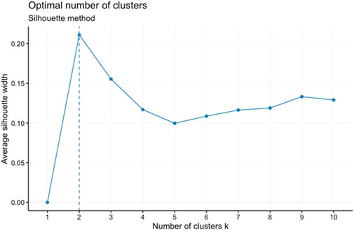
FIGURE 1. Silhouette method testing the best number of clusters to set for the k-means algorithm given the chlorite element chemistry data. In this case, the optimal number of clusters is two.
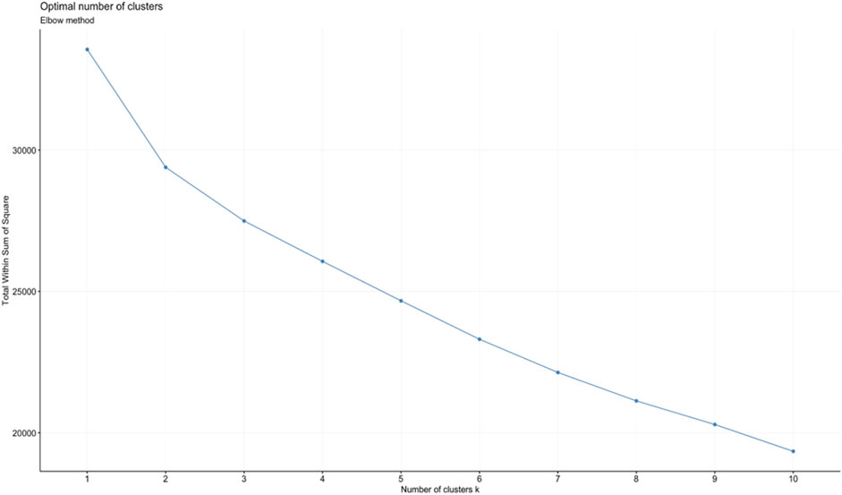
FIGURE 2. Plot of the elbow method showing the total WSS for different numbers of clusters. Tested with the chlorite element chemistry data for the k-means clustering algorithm. The plot shows the optimal number of clusters indicated by the “elbow” which occurs at k = 2.
The two clustering algorithms were performed on the scaled data; for k-means 50 iterations were used. To compare the clustering results with the environmental/geological properties of the data themselves, our data were grouped into bins based on their distance from a hydrothermal center. Different amounts and ranges of bins were compared with the clustering results to assess different outcomes. Most of the ranges of the bins were determined to spread out the distance data somewhat equally. From the filtered and trimmed 2,942 analyses, the minimum and maximum distances to the respective deposit center was 5.5 and 19,051 m respectively.
For the k-means algorithm, runs of different ranges of four and five bins were created. The first run used four bins based on the 25th, 50th and 75th percentiles of the 2,942 distance data points (i.e., d ≤ 1,375; 1,375 < d ≤ 1,813; 1,813 < d ≤ 3,682; d > 3,682). Other bins and ranges were varied to test what natural groupings of data could be found that also provide useful distances from mineralization (Table 1).
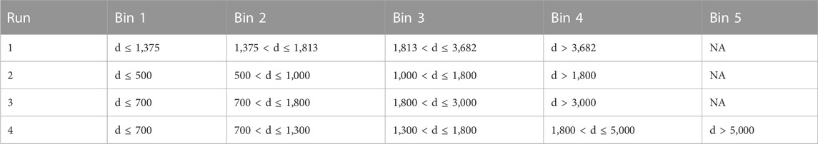
TABLE 1. Runs of bins and their associated ranges tested in the k-means algorithm. The bins of run 1 are defined by the 25th, 50th and 75th percentiles of the 2,942 distance data points. Bins from runs 2–4 were defined arbitrarily to test how differently data separates under different bins.
For hierarchical clustering, runs 1 and 3 were used as well as some additional runs with new bins. The new bins were created by splitting the first bin of the percentile-determined bins in different ways. This is summarized in Table 2. After hierarchical clustering of the entire data set hierarchical cluster analysis was also performed on the data set using only trace elements and major elements that did not vary based on parent mineral (Co, Cr, Cu, Li, Ni, Pb, Si, Sn, Sr, Ti, V, Y, and Zn) to test whether by utilizing only these elements the effects of inheritance of trace elements from the mineral the chlorite is replacing could be avoided.
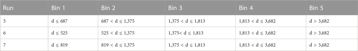
TABLE 2. Additional runs tested against the hierarchical clustering algorithm. Bin 1 of runs 5–7 is less than or equal to half of the 25th percentile, 12.5th percentile, and 18th percentile respectively. Bin 2 is between these values and the 50th percentile. Bins 3–5 remain the same as bins 2–4 from run 1.
Lastly, independent hierarchical cluster analyses were conducted on data from two different deposits. One used data from the Northparkes district and one used data from the Batu Hijau district. Both used all elements and the same methodology described above.
Results
K-means
The k-means clustering algorithm was performed with k = 2, resulting in two clusters. The various runs of distinct bins allow for different views and interpretations of the clustering results. Figure 3A shows the clustering results compared against the 25th, 50th, and 75th percentile distance bins (run 1). Cluster 1 consists mostly of chlorite further away from the deposit center (85% of the analyses in cluster 1 are from >1,813 m from the deposits), whereas cluster 2 contains more proximal chlorite (70% of analyses in cluster 2 are from <1,813 m from the deposits). Albeit some overlap occurs in both clusters, as the two nearest and furthest bins are not perfectly segregated from each other, but the results show a general separation between proximal and distal chlorite. Figure 3B shows the same clustering results compared against the bins of run 2. The range of these bins are compressed in comparison to those in Figure 3A (run 1). With a narrower range of bins, cluster 1 now comprises most of one bin (85% of chlorite analyses are from greater than 1,800 m away from the deposit center), whereas cluster 2 contains a significant amount of each bin. There is more overlap in Figure 3B and not as clear of a distinction between the proximal and distal bins. Figure 3C compares the clustering results with the set of bins from run 3, which are broader than in Figure 3B (run 2) but still narrower than in Figure 3A (run 1). Similar to Figure 3B, cluster 1 still comprises mostly samples from the furthest bin, however there are more analyses from the second most distal bin as well (70% of analyses in cluster 1 >3,000 m from the deposits and 15% from 1,800 to 3,000 m from the deposit). Cluster 2 contains analyses from all four bins, similar to the results in Figure 3B. Figure 3D compares the clustering results binned by run 4, which has a set of five distance bins. All the figures and binning schemes show a small portion of the most proximal chlorite grouped in cluster 1, where most of the distal chlorite reside. For example, 14% of the chlorite in the most proximal distance bin in Figure 3A is grouped in cluster 1. There is also some chlorite from the most distal bin grouped with the nearer bins in cluster 2. Although there exists some overlap in the clusters among the different bins, overall, there is somewhat of a distinction between proximal and distal chlorite in the clusters.
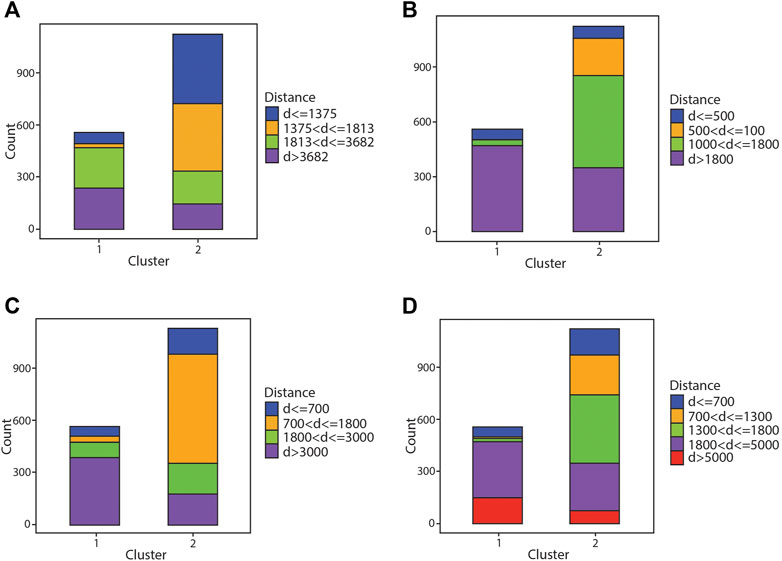
FIGURE 3. Bar graph showing results of the k-means clustering algorithm compared against different distance bins. (A) Comparison of results with quartile distance bins. (B–D) Comparison of results against narrower distance bins.
Hierarchical
The hierarchical clustering algorithm was performed using different k values, because the elbow method and silhouette method gave no clear indication of an optimal k value. Because of this 2, 3, and 4 clusters were tested against different bins. Figure 4 shows scatter plots of trace elements with results of hierarchical clustering and distance to mineralization. Figure 5A shows the clustering results compared against the 25th, 50th, and 75th percentiles distance bins (run 1). The chlorite data seems to be spread more evenly among the two clusters in this run using the hierarchical algorithm. Cluster 1 contains most chlorite from the two most proximal bins (77% of cluster 1), with some inclusion of chlorite from the two most distal bins. The two most distal chlorite bins are grouped mostly within cluster 2 (79% of the analyses from >1,813 m in cluster 2), with some overlap as well from the two most proximal bins. Although significant overlap of the bins is present in run 1, the hierarchical algorithm better separates proximal chlorite from distal chlorite than from the k-means algorithm in Figure 3A.
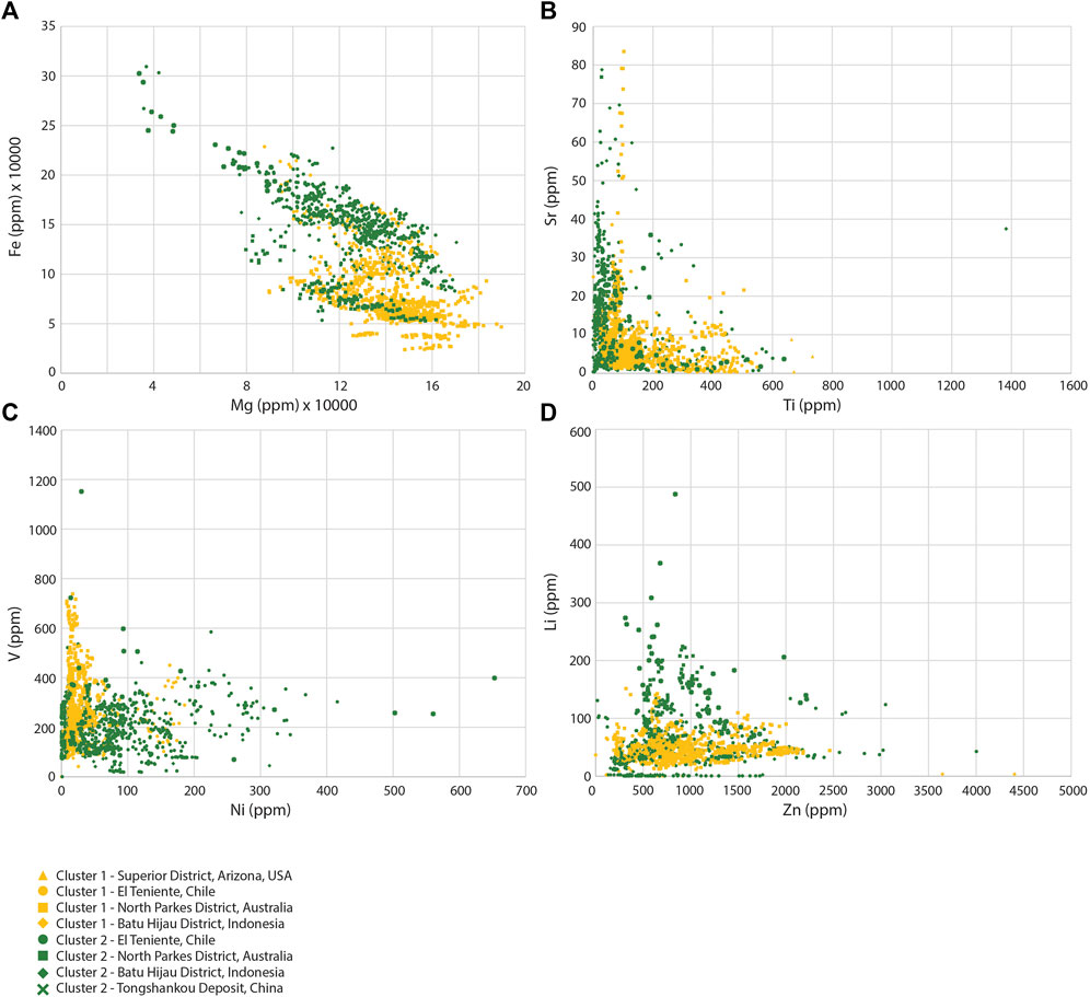
FIGURE 4. Results of the hierarchical clustering algorithm. Clusters are given by the color and deposit are given by the shape. (A) Fe vs. Mg, (B) Sr vs. Tl, (C) V vs. Ni, and (D) Li vs. Zn.
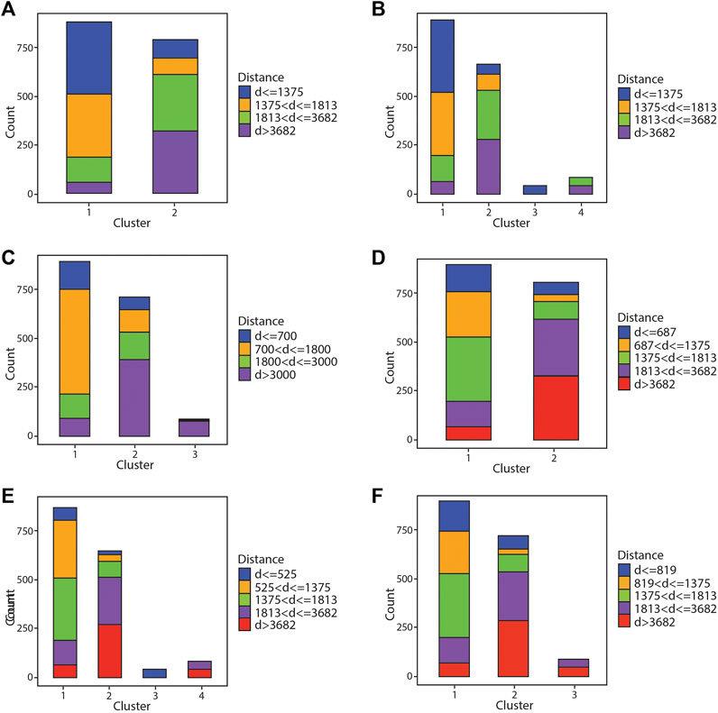
FIGURE 5. Bar graph showing results of the hierarchical clustering algorithm compared against different distance bins. (A,B) Comparison of results against quartile distance bins with two and four clusters, respectively. (C–F) Comparison of results against narrower distance bins with varying number of clusters.
Figure 5B shows run 1 again but split across four clusters (k = 4). Ideally the four chlorite bins would segregate into their own cluster, however in these results there is significant contribution from each group in 2 of the 4 clusters. Cluster 3 consists primarily of the most proximal chlorite bin, with minor inclusions of the second most proximal bin. Cluster 1 consists more of the two most proximal chlorite bins (74% of cluster 1 < 1,813 m), while grouping some of the distal chlorite in as well. Cluster 2 contains predominantly chlorite from the two most distal bins (79% of cluster 2 > 1,813 m), with some overlap from the two most proximal bins, while cluster 4 is almost entirely chlorite from the two most distal bins. There is clear segregation of the proximal and distal chlorite across clusters 3 and 4, whereas clusters 1 and 2 contain overlap across all bins.
Figure 5C shows groupings of the data from hierarchical clustering with k = 3 of run 3. There is good segregation of chlorite from the most distal bin in cluster 3, however in cluster 2 there is significant overlap across all bins albeit the majority is chlorite from the two most distal bins (74% of cluster 2 from analyses >1,813 m). Cluster 1 also contains most of the chlorite from the two most proximal bins (75% from <1,813 m), and again, some overlap is still seen from the groupings of chlorite in the two most distal bins.
Figure 5D shows the clustering results against run 5 with two clusters. This shows similar results to Figure 5A, where cluster 1 and cluster 2 seem to segregate proximal chlorite and distal chlorite respectively, yet both clusters still contain some minor overlap with one another.
Figure 5E shows the results of run 6 using 4 clusters. These results are similar to Figure 5B. Again, there is a cluster containing solely chlorite from the most proximal bin, and another cluster with chlorite from the most distal bins, clusters 3 and 4 respectively. Cluster 1 consists mostly of chlorite from the proximal bins (77% of the analyses from <1,813 m), yet still grouping a smaller portion of chlorite from the distal bins. This is seen for cluster 2 as well, but distal chlorite dominates with less inclusions of proximal chlorite (79% of analyses from >1,813 m).
Figure 5F shows the clustering results compared against bins from run 7 using 3 clusters. This depicts similar results to Figure 5C. Cluster 3 segregates solely a portion of chlorite from the two most distal bins, however chlorite from these bins are still present in clusters 1 and 2. Cluster 1 is able to mostly differentiate proximal chlorite from distal (79% of analyses from <1,813 m), but still incorporates some chlorite from the distal bins. This is seen in cluster 2 but with distal chlorite dominating (74% of analyses from >1,813 m). In all, comparing the clustering results across different algorithms and bins, most results show somewhat of a segregation between proximal and distal chlorite but cannot fully differentiate them as the clusters depict a portion of overlap across all bins.
Additionally, when investigating the deposits individually, there appears to be bias in the interpretation when only distance to deposit is investigated in the different clusters. The classifier separates the deposits based on metal contained within the deposit with the same or better segregation than distance to the deposit. The analyses from Cu-Au deposits make up 91% of cluster 1 while the analyses from Cu-Mo deposits make up 76% of cluster 2 (Table 3).
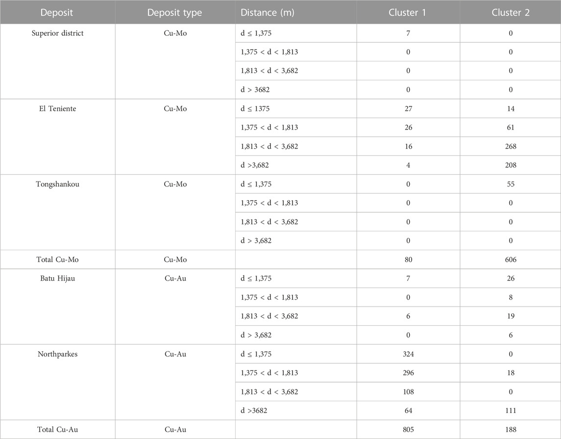
TABLE 3. Hierarchical clustering results for each deposit and distance to deposit.
An additional cluster analysis was conducted using only trace elements and major elements less dependent on parent mineral (Co, Cr, Cu, Li, Ni, Pb, Si, Sn, Sr, Ti, V, Y, and Zn). This gave relatively poor results in that the majority of the analyses were contained within cluster 1 (80% in cluster 1). While the majority of the analyses in cluster 2 were from the samples from greater distance to the deposit (85% of analyses in cluster 2 from >1,810 m from the deposit), approximately twice as many analyses from these distances were grouped into cluster 1 (Table 4).
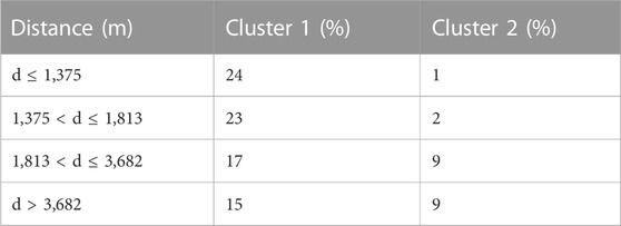
TABLE 4. % of analyses from each distance in each cluster when hierarchical cluster completed with only trace elements.
The cluster analysis of the individual deposits (Northparkes and Batu Hijau districts) was less successful (Figure 6). While they did generally separate the distal samples preferentially into cluster 2 (100% of analyses in cluster 2 are from >3,681 m at Northparkes and 47% of analyses in cluster 2 from Batu Hijau from >3,681 m) most of the analyses from both deposits were grouped into cluster 1 (88% of analyses from Northparkes in cluster 1 and 83% of analyses from Batu Hijau in cluster 1).
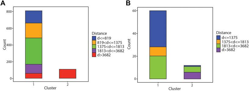
FIGURE 6. Bar graph showing results of the hierarchical clustering algorithm for individual deposits. (A) gives results for samples from the Northparkes district and (B) gives results for the Batu Hijau district.
Discussion
The segregation of the chlorite bins depends heavily on how the bins are assigned; however, in comparing all of the clustering outcomes across different algorithms and bins, most results show some degree of segregation between proximal and distal chlorite. Yet, the clustering results are unable to fully differentiate chlorite proximity to ore body into distinct clusters and there is a portion of overlap across all distances of chlorite deposition. This may be due in part to the difficulty in clearly defining how far a given sample is from a deposit and thereby be the result of biases within chlorite data collection and recording. The most optimal results are depicted from the hierarchical and k-means algorithms with two clusters under the quartile distance bins as they show the best segregation between proximal and distal chlorite (Figures 3A, 5A), with the least amount of overlap. This could have been influenced by the evenly distributed chlorite data across each bin, or perhaps the distances defined in each bin represent the bounds of different alteration halos surrounding the center of the deposits that define a new geochemical signature of the chlorite. Another important observation is noted amongst the k-means results from the runs with the narrower bins (Figures 4B–D); these show a significant portion of the most proximal chlorite samples grouping with the cluster dominated by the most distal chlorite bin. Perhaps some of the distal chlorite has a low-grade metamorphic imprint that results in a trace element chemistry similar to the proximal hydrothermal chlorite. Further studies can be dedicated to investigating any further imprint of metamorphism on the chlorite data using magnesium-to-iron ratios to differentiate metamorphic chlorite from hydrothermal chlorite as to avoid as much skewing of the clustering results as possible (Kamps et al., 2018). We further tested whether cluster analyses using only trace elements and major elements less dependent on the primary mineral might be more effective than cluster analyses that contain major elements such as Fe and Mg (Table 4). These were unsuccessful as the majority of analyses were contained within cluster 1, limiting the use of trace element only cluster analysis as a vectoring tool. This demonstrates that the major elements, including Fe and Mg, which are inherited from primary minerals are important components of chlorite chemistry as a vector towards mineralization.
Previous studies have explored the application of chlorite chemistry as a vector towards an ore deposit center (Chu et al., 2020; Cooke et al., 2020; Wilkinson et al., 2015 amongst others). These studies investigated one- and/or two-dimensional trends of trace element behavior in chlorite for a single deposit. Although there were substantial trends in certain element variations at different distances away from the deposit center in these studies, these were deposit-specific and did not consider trends in chlorite’s entire trace element composition as a whole. Machine learning algorithms applied in this study were able to identify similarities in several trace element concentrations in chlorite at varying distances away from mineralization. Using multi-dimensional chlorite chemistry data from different deposits allows for investigating its use as a vector on a universal level. The results of the unsupervised learning algorithms show that there exists a similarity in how trace element concentrations behave within chlorite from different deposits at varying distances away. Albeit the results from the clustering do not perfectly segregate the different chlorite bins, there is still significant segregation between them. The data shows a good distinction of proximal chlorite from distal chlorite, suggesting that chlorite chemistry is potentially unique at different distances away from a deposit center. However, these results are partially an artifact of differences in the geology of the deposits. The data set used here is dominated by analyses of chlorite from Cu-Mo (Superior district, El Teniente, and Tongshankou) and Cu-Au (Northparkes district and Batu Hijau) porphyry systems. Of these the data set contains more analyses from El Teniente (dominated by distal samples) and Northparkes (dominated by proximal samples). When looked at in detail the the metals contained in the deposits appear to have a greater control on which cluster the chlorite analyses are grouped in that 81% of the analyses from Cu-Au deposits are in cluster 1 and 88% of the analyses from Cu-Mo deposits are in cluster 2 (Table 3). This suggested that the development of a universal classifier using cluster analysis is unlikely to be effective and that independent classifiers should be developed for each different porphyry type. To test the efficacy of such a classifiers cluster analysis was performed on two individual deposits (Batu Hijau and Northparkes). This was determined to be significantly less effective, and the majority of the data was grouped into one of the clusters limiting the cluster analysis’ use as a vectoring tool in such an environment (Figure 6). This suggests that cluster analysis of chlorite chemistry is not an effective method to develop a universal vector towards porphyry mineralization.
Limitations of study
Naturally, conducting studies on compilations of data from a number of studies has certain limitations. First, the measure of distance of the samples from the ore deposit is subjective. Because ore deposits are not of uniform dimensions and what is defined as “ore” will vary depending on economic factors in addition to physical factors the measure of the distance to a deposit will vary from place to place. Further, the direction of the distance from the ore deposit is likely to also be variable and would affect the amount and source of fluids that interacted with the rock. For example, 500 m above a porphyry system will have different fluid conditions to 500 m adjacent to a porphyry system. Because these details are difficult to resolve when studying a site in detail, they are even more difficult to correct when compiling data and are limitations of this study.
Additionally, differences in the collection of the LA-ICPMS data can also lead to limitations in the data compilations. Different labs may utilize different instruments, different tuning procedures, different standard materials, and different internal standards when conducting data reduction. Changes in each of these could affect the output data and could result in errors when interrogating the compiled data set.
Conclusion
Unsupervised machine learning algorithms serve as a multi-dimensional approach in investigating the potential of chlorite chemistry as a vector towards mineralization. There are significant groupings of proximal chlorite from distal chlorite that suggests a use of chlorite’s trace element chemistry as a proxy for vectoring towards a deposit center. However, the utility of this as an universal vector are somewhat diminished in that it is only able to separate analyses from >1,800 m from a deposit from those <1,800 m from a deposit. Further, these results are likely more based on metals contained in the deposits rather than distance to the deposit center, indicating that cluster analysis of chlorite trace element chemistry is unlikely to be a useful vector towards porphyry mineralization. Next steps would involve obtaining a larger database that considers chlorite from more porphyry and/or hydrothermal deposits to be able to assess whether there is a clear universal trend in trace element behavior in chlorite.
Data availability statement
Publicly available datasets were analyzed in this study. This data can be found here: Doi: 10.26022/IEDA/112228 EarthChem Library.
Author contributions
NF—collected the data, filtered the data, conducted the cluster analyses, wrote the paper. DG—designed the project, supervised the project, edited the paper. SM—aided and provided input for the project and edited the paper. SZ—aided and provided input for the project and edited the paper. All authors contributed to the article and approved the submitted version.
Conflict of interest
The authors declare that the research was conducted in the absence of any commercial or financial relationships that could be construed as a potential conflict of interest.
Publisher’s note
All claims expressed in this article are solely those of the authors and do not necessarily represent those of their affiliated organizations, or those of the publisher, the editors and the reviewers. Any product that may be evaluated in this article, or claim that may be made by its manufacturer, is not guaranteed or endorsed by the publisher.
References
Banerjee, A., and Dave, R. N. (2004). “Validating clusters using the Hopkins statistic,” in 2004 IEEE International conference on fuzzy systems (IEEE Cat. No. 04CH37542) (IEEE) 1, 149–153.
Camus, F. (2002). “The Andean porphyry systems,” in Super porphyry copper and gold deposits: A global perspective. Editor T. M. Porter 1st ed. (Adelaide: PGC Publishing), 45–63.
Cannell, J., Cooke, D. R., Walshe, J. L., and Stein, H. (2005). Geology, mineralization, alteration, and structural evolution of the El Teniente porphyry Cu-Mo deposit. Econ. Geol. 100, 979–1003. doi:10.2113/gsecongeo.100.5.979
Chu, G., Zhang, S., Zhang, X., Xiao, B., Han, J., Zhang, Y., et al. (2020). Chlorite chemistry of Tongshankou porphyry-related Cu–Mo–W skarn deposit, Eastern China: implications for hydrothermal fluid evolution and exploration vectoring to concealed orebodies. Ore Geol. Rev. 122, 103531. doi:10.1016/j.oregeorev.2020.103531
Cooke, D. R., Wilkinson, J. J., Baker, M., Agnew, P., Phillips, J., Chang, Z., et al. (2020). Using mineral chemistry to aid exploration: A case study from the resolution porphyry Cu-Mo deposit, Arizona. Econ. Geol. 115 (4), 813–840. doi:10.5382/econgeo.4735
Deer, W. A., Howie, R. A., and Zussman, J. (2013). An introduction to the rock-forming minerals. London: The Mineralogical Society.
Dmitrijeva, M., Cook, N. J., Ehrig, K., Ciobanu, C. L., Metcalfe, A. V., Kamenetsky, M., et al. (2020). Multivariate statistical analysis of trace elements in pyrite: prediction, bias and artefacts in defining mineral signatures. Minerals 10 (1), 61. doi:10.3390/min10010061
Freij, N., Gregory, D. D., and Lui, Y. (2023). A data screening approach to confirming a target mineral is chlorite using EPMA and LA-ICPMS data. Geoscience Data J. doi:10.1002/gdj3.190
Fulignati, P. (2020). Clay minerals in hydrothermal systems. Minerals 10 (10), 919. doi:10.3390/min10100919
Imai, A., and Ohno, S. (2008). Primary ore mineral assemblage and fluid inclusion study of the Batu Hijau porphyry Cu-Au deposit, sumbawa, Indonesia. Resour. Geol. 55, 239–248. doi:10.1111/j.1751-3928.2005.tb00245.x
Kamps, O. M., Van Ruitenbeek, F,J,A., Mason, P. D. R., and Van der Meer, F. D. (2018). Near-infrared spectroscopy of hydrothermal versus low-grade metamorphic chlorites. Minerals 8 (6), 259. doi:10.3390/min8060259
Krynen, J. P., Sherwin, L., and Clarke, I. (1990). Stratigraphy and structure. Rec. Geol. Surv. N. S. W. 23, 1–76.
Lickfold, V., Cooke, D. R., Crawford, A. J., and Fanning, C. M. (2007). Shoshonitic magmatism and the formation of the Northparkes porphyry Cu-Au deposits, New South Wales. Aust. J. Earth Sci. 54, 417–444. doi:10.1080/08120090601175754
Pacey, A., Wilkinson, J. J., and Cooke, D. R. (2020). Chlorite and epidote mineral chemistry in porphyry ore systems: A case study of the Northparkes district, New South Wales, Australia. Econ. Geol. 115 (4), 701–727. doi:10.5382/econgeo.4700
Pacey, A., Wilkinson, J. J., Owens, J., Priest, D., Cooke, D. R., and Millar, I. L. (2019). The anatomy of an alkalic porphyry Cu-Au system: geology and alteration at Northparkes mines, New South Wales, Australia. Econ. Geol. 114, 441–472. doi:10.5382/econgeo.4644
R Core Team (2020). R: A language and environment for statistical computing. Vienna, Austria: R Foundation for Statistical Computing. URL. Available at: https://www.R-project.org/.
Rio Tinto (2018). Annual report. Available at: www.riotinto.com/documents/RT_2018_annual_report.pdf.
Rousseeuw, P. J. (1987). Silhouettes: A graphical aid to the interpretation and validation of cluster analysis. J. Comput. Appl. Math. 20, 53–65. ISSN 0377-0427. doi:10.1016/0377-0427(87)90125-7
Sillitoe, R. H. (2010). Porphyry copper systems. Econ. Geol. 105 (1), 3–41. doi:10.2113/gsecongeo.105.1.3
Sillitoe, R. H. (1973). The tops and bottoms of porphyry copper deposits. Econ. Geol. 68 (6), 799–815. doi:10.2113/gsecongeo.68.6.799
Simpson, C. J., Cas, R. A. F., and Arundell, M. C. (2005). Volcanic evolution of a long-lived Ordovician island-arc province in the Parkes region of the Lachlan fold belt, southeastern Australia. Aust. J. Earth Sci. 52, 863–886. doi:10.1080/08120090500304273
Skewes, A. M., Arévalo, A. G., Floody, R., Zúñiga, P., and Stern, C. R. (2002). The giant El Teniente breccia deposit: hypogene copper distribution and emplacement. Soc. Econ. Geol. Special Publ. 9, 299–332. doi:10.5382/SP.09.14
Thorndike, R. L. (1953). Who belongs in the family? Psychometrika 18, 267–276. doi:10.1007/BF02289263
Wang, Y., Fan, H., Pang, Y., and Xiao, W. (2022). Geochemical characteristics of chlorite in xiangshan uranium ore field, South China and its exploration implication. Minerals 12 (6), 693. doi:10.3390/min12060693
Wilkinson, J. J., Baker, M. J., Cooke, D. R., and Wilkinson, C. C. (2020). Exploration targeting in porphyry Cu systems using propylitic mineral chemistry: A case study of the El Teniente deposit, Chile. Econ. Geol. 115 (4), 771–791. doi:10.5382/econgeo.4738
Wilkinson, J. J., Chang, Z., Cooke, D. R., Baker, M. J., Wilkinson, C. C., Inglis, S., et al. (2015). The chlorite proximitor: A new tool for detecting porphyry ore deposits. J. Geochem. Explor. 152, 10–26. ISSN 0375-6742. doi:10.1016/j.gexplo.2015.01.005
Keywords: cluster analysis, porphyry, chlorite, LA-ICPMS, trace element, vector, hierarchical, k-mean algorithm
Citation: Freij N, Gregory DD, Zhang S and Morrison SM (2023) Chlorite geochemical vectoring of ore bodies: a natural kind clustering approach. Front. Earth Sci. 11:1222291. doi: 10.3389/feart.2023.1222291
Received: 14 May 2023; Accepted: 03 August 2023;
Published: 17 August 2023.
Edited by:
Jaroslaw Majka, Uppsala University, SwedenReviewed by:
Franck Bourdelle, CY Cergy Paris Université, FranceJesse Walters, Goethe University Frankfurt, Germany
Marek Szczerba, Polish Academy of Sciences, Poland
Copyright © 2023 Freij, Gregory, Zhang and Morrison. This is an open-access article distributed under the terms of the Creative Commons Attribution License (CC BY). The use, distribution or reproduction in other forums is permitted, provided the original author(s) and the copyright owner(s) are credited and that the original publication in this journal is cited, in accordance with accepted academic practice. No use, distribution or reproduction is permitted which does not comply with these terms.
*Correspondence: Daniel David Gregory, ZGFuaWVsLmdyZWdvcnlAdXRvcm9udG8uY2E=