Interpretable machine learning model for shear wave estimation in a carbonate reservoir using LightGBM and SHAP: a case study in the Amu Darya right bank

The shear wave velocity (Vs) is significant for quantitative seismic interpretation. Although numerous studies have proved the effectiveness of the machine learning method in estimating the Vs using well-logging parameters, the real-world application is still hindered because of the black-box nature of machine learning models. With the rapid development of the interpretable machine learning (ML) technique, the drawback of ML can be overcome by various interpretation methods. This study applies the Light Gradient Boosting Machine (LightGBM) to predict the Vs of a carbonate reservoir and uses the Shapley Additive Explanations (SHAP) to interpret the model. The application of ML in Vs estimation normally involves using conventional well-log data that are highly correlated with Vs to train the model. To expand the model’s applicability in wells that lack essential logs, such as the density and neutron logs, we introduce three geologically important features, temperature, pressure, and formation, into the model. The LightGBM model is tuned by the automatic hyperparameter optimization framework; the result is compared with the Xu-Payne rock physics model and four machine learning models tuned with the same process. The results show that the LightGBM model can fit the training data and provide accurate predictions in the test well. The model outperforms the rock physics model and other ML models in both accuracy and training time. The SHAP analysis provides a detailed explanation of the contribution of each input variable to the model and demonstrates the variation of feature contribution in different reservoir conditions. Moreover, the validity of the LightGBM model is further proved by the consistency of the deduced information from feature dependency with the geological understanding of the carbonate formation. The study demonstrates that the newly added features can effectively improve model performance, and the importance of the input feature is not necessarily related to its correlation with Vs

1 Introduction

Shear wave velocity (Vs) is one of the most crucial elastic parameters for quantitative seismic interpretation as it provides useful petrophysical, lithological, and geomechanical information (Greenberg and Castagna, 1992; Rezaee et al., 2007; Anemangely et al., 2017; Olayiwola and Sanuade, 2021). Sonic logging is the most accurate way to measure the shear velocity in subsurface formations, while due to the high cost and time constraints, Vs logging is often unavailable in most fields (Wang et al., 2020; Miah, 2021). Consequently, attempts with various approaches have been made in estimating the Vs using petrophysical loggings.

The empirical formula method is the most common approach to first estimate the shear wave velocity by constructing a linear relationship between logging parameters and Vs (Castagna et al., 1985; Han et al., 1986; Dvorkin, 2008; Parvizi et al., 2015). However, the empirical relationship is highly lithology- and region-specific (Tamunobereton-Ari et al., 2010). In carbonate formation, which has a complex pore structure and strong heterogeneity, the variation of shear wave velocity in carbonate is the result of an interaction between lithofacies, diagenetic process, and porosity (Rafavich et al., 1984; Anselmetti and Eberli, 1993; Tamunobereton-Ari et al., 2010; Qabany et al., 2011; Wang et al., 2011; Kittridge, 2015; Garia et al., 2019). Thus, simple linear approximation is insufficient for accurately estimating the Vs The rock physics modeling technique for carbonate has being extensively studied by considering different mineral types, pore structures, and fluid conditions, and the studies have shown promising results (Xu and Payne, 2009; Sun et al., 2012; Zhang et al., 2013; Azadpour et al., 2020; Seifi et al., 2020). However, the modeling process requires pore structure quantification and the accurate interpretation of petrophysical parameters and lithofacies, which needs to be calibrated by vast amounts of laboratory tests from rock samples before use. However, the conditions are not always met, causing the instability of predictions from the rock physics model.

The data-driven approach, such as machine learning (ML), has received great attention due to its strong ability in building non-linear relationships between input variables and the target. ML has been prevalently used in well logging interpretation of petrophysical and geomechanical parameters. Numerous studies have demonstrated the reliable application in shear wave velocity estimation in carbonate formation using different algorithms, e.g., neural-network based model (Hadi and Nygaard, 2018; Alkinani et al., 2019; Mehrgini et al., 2019; Zhang et al., 2020; 2022; Ebrahimi, 2022; Mehrad et al., 2022; Rajabi et al., 2022; Taheri et al., 2022), support vector machine (Bagheripour et al., 2015; Anemangely et al., 2019), tree-based model (Zhong et al., 2021), fuzzy inference system (Nourafkan and Kadkhodaie-Ilkhchi, 2015), and clustering algorithm (Alameedy et al., 2022). Despite the plentiful research on this subject, the use of machine learning is still hindered by its black box nature, which makes it difficult to understand how the output is achieved. The reason is that the machine learning models are usually trained by a vast amount of data and they can be highly complex to interpret (Du et al., 2019; Murdoch et al., 2019; Roscher et al., 2020; Belle and Papantonis, 2021; Molnar et al., 2021). In a regression task like shear wave estimation, such a drawback limits the choices of input features during the training process, i.e., only loggings that are considered geologically meaningful or highly correlated with shear wave velocity, like compressional wave velocity (Vp), are chosen to build the model. New features that can increase the model performance can hardly be introduced into the model without explaining the feature importance and contribution by reliable interpretation tools.

Interpretable or explainable machine learning (IML) has received great attention nowadays in response to the booming complexity of machine learning models; the method can be employed for model validation, model debugging, or knowledge discovery (Du et al., 2019; Rudin et al., 2022). Numerous interpretation approaches have been proposed, which can fall into two categories: model-specific and model-agnostic. Model-specific methods are specifically designed for different methods, such as weights for explaining the feature importance in generalized linear models (Nelder and Wedderburn, 1972), while model-agnostic methods are general schemes that can be applied to various models to provide insight into feature importance, e.g., permutation feature importance for evaluating the contribution of certain features to the overall model performance (Altmann et al., 2010). Both types of IML have been widely utilized in areas such as the prevention of geological hazards (Dikshit et al., 2021; Ma et al., 2022), biochemistry (Vellido, 2020; Esterhuizen et al., 2022), and civil engineering (Feng et al., 2021).

In this study, we train a LightGBM regression model to predict the shear wave velocity, and the model can be applied in the development wells where logging type is limited. To compensate the model performance reduction caused by the lack of crucial loggings, we added three new features into the model and adopted the model-specific TreeSHAP method to quantitatively demonstrate the effectiveness and reliability of the newly added features (Lundberg and Lee, 2017; Lundberg et al., 2018). We targeted the low permeability porous carbonate reservoir in a gas field located on the right bank of the Amu Darya river. The gas field is covered by three appraisal wells with a comprehensive well-logging set and three development wells with density and neutron logs missing. To increase the prediction accuracy, we conducted the feature engineering technique and added three more features into the model, namely, temperature, pressure, and formation information. With the help of the automatic hyperparameter optimization technique, the LightGBM model is compared with four classic machine learning models that are frequently used in the regression task and the Xu-Payne rock physics model. Moreover, we fully analyze the model output using TreeSHAP, both globally and locally, to demonstrate how the predictions are made, how each feature contributes to the final prediction, and the usefulness of the newly added features. The results show that new features can compensate for the loss of crucial loggings and effectively increase the model accuracy and generalization ability. Compared with other machine learning and rock physics modeling methods, the LightGBM model can provide accurate results efficiently, especially in areas that have complex lithology, high clay content, and high porosity, which often cause unreliable predictions in the Xu-Payne model.

2 Reservoir characteristics

The right bank of Amu Darya is located at the eastern border of Turkmenistan, closely adjacent to Uzbekistan (Figure 1). After a series of tectonic evolutions from the Permian to the Holocene, the current geological framework can be separated into six structure belts: the Chardzhou step, Kennedykiddskurt uplift, Carlabekaul depression, Sandykly uplift, Bieshikent depression, and Gissar predominant thrust belt (Tian et al., 2016; Shan et al., 2022; Wu et al., 2022). The gas field D, which geologically belongs to the Chardzhou step, is located at the northwestern part of the block (Figure 1).

FIGURE 1

FIGURE 1. Location of the Amu Darya Right Bank. The study area (gas field D) is indicated by the red rectangle.

The Callovian-Oxfordian carbonate formation, which has a thickness of approximately 400 m, is divided into eight layers, labeled XVac, XVp, XVm, XVhp, XVa1, Z, XVa2, and XVI. It is considered as a major hydrocarbon reservoir that is controlled by depositional and diagenetic processes (Liu et al., 2013; Xing et al., 2022). In the early Callovian, a major transgression occurred and formed the mixed shelf sedimentary environment (Wu et al., 2019). Then a series of argillaceous limestone interlayered with thin calcareous mudstone that has high Gamma Ray (GR) values were deposited at the inner ramp. The low energy environment in the inner ramp has little hydrodynamic differentiation effect on the sediments and causes the formation of the mound-beach complexes on the geomorphological high point. During the Oxfordian, the ramp went through a transgression and being submerged, constructed a rimmed platform in the middle of the Kennedykiddskurt uplift. After the deposition of the XVhp formation, the aggradation of reef-shoal complex continues on top of the previously deposited mound-beach complexes. The deposition of carbonates ends with a large-scale regression during the late Oxfordian and early Tithonian; then, the increasing brine concentration leads to a long period of precipitation of gypsum and salt (Figure 2).

FIGURE 2

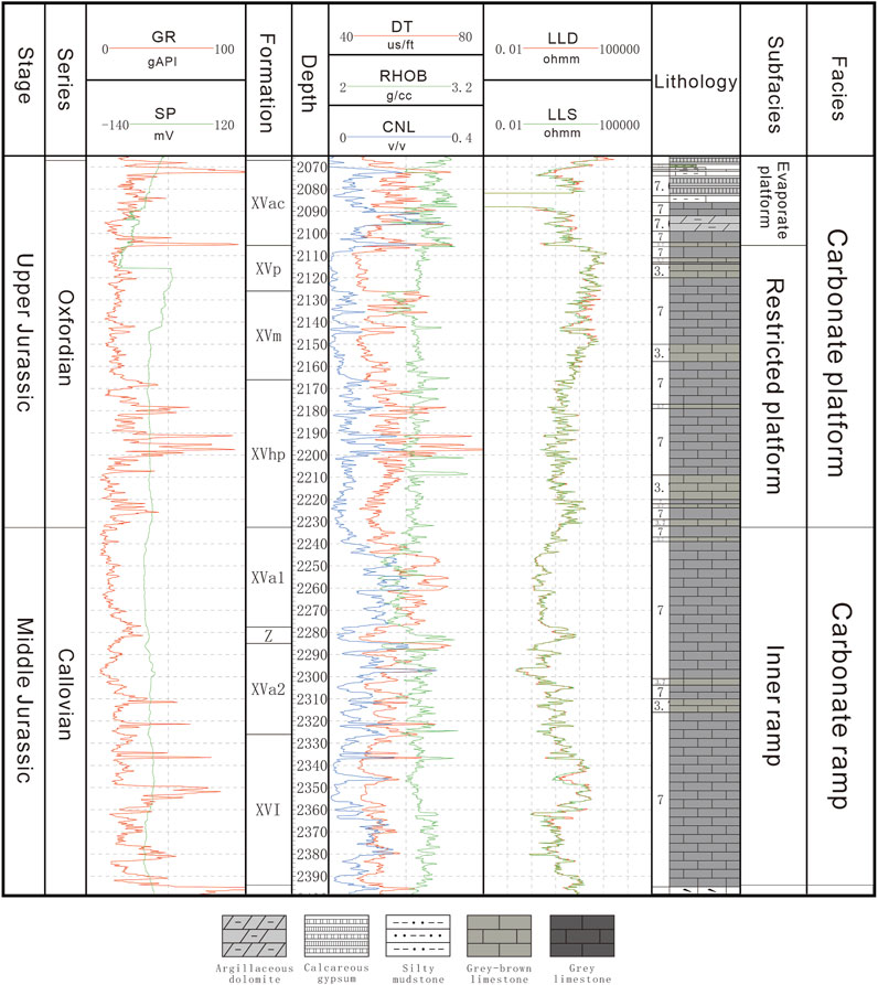
FIGURE 2. The stratigraphy of the Callovian-Oxfordian formation and well logs of JE1.

The dominating lithofacies in the Callovian-Oxfordian carbonates are bioclast limestone, oolitic limestone, and micrite limestone, which associated with characteristic shoal facies within the platform. The reservoir lithofacies are mainly composed of microcrystalline sandy oolitic limestone, sparry oolitic limestone, pellet microcrystalline limestone, and powder crystalline limestone (Figures 3A–C). The sedimentary environment variation during the deposition of XVac caused the layer to become interfingered with thin gypsum and dolomite, which can be observed in the mudlog in Figure 2.

FIGURE 3

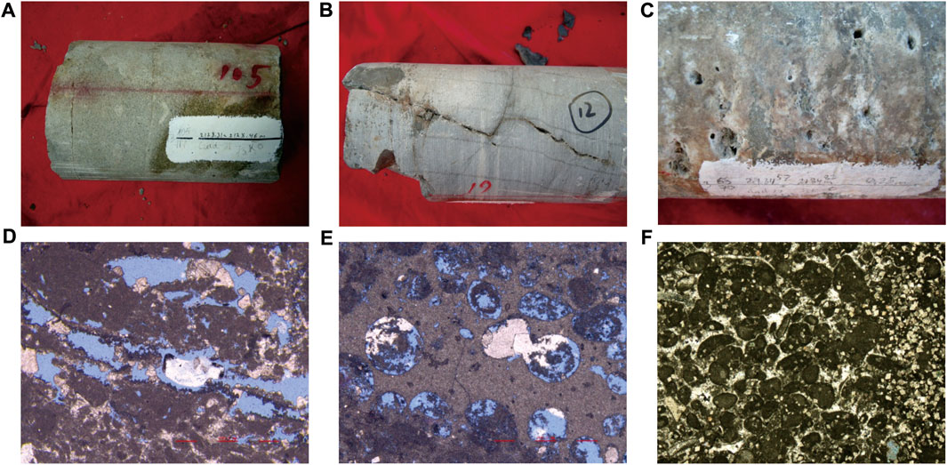
FIGURE 3. Core and thin-section observation of samples from upper three layers (A) JE1, 2128.40 m, XVm, light grey fine-grained limestone. (B) JE1, 2106 m, XVp, powder crystalline limestone with fracture, half-filling by mud. (C) JE2, 2184 m, XVp, brown-gray micrite limestone with a developed cave. (D) BJE1, 2167.4 m, XVac, gastropod micrite limestone. (E) BJE1, 2147.61 m, XVac, deformed micrite sandy oolitic limestone. (F) JE1, 2131 m, XVm, sparry oolitic limestone.

The major storage space for the hydrocarbon are secondary and residual primary pores; only a small proportion of fractures and dissolution caves are developed. The dissolved and residual primary pores can be found in grainstone and bioclastic limestone, and the grain surface is often covered with sparry calcite (Figures 3D–F). The dissolved pores inside grains are often developed in microcrystalline sandy limestone; sometimes the grain is totally dissolved and leaves a moldic pore. The small number of fractures developed in XVp and XVm often have high angles and are partially cemented with mud (Figure 3B). The distribution of dissolving caves is heterogeneous and mostly associated with fractures; the maximum width of caves is 3 mm (Figure 3C).

3 Data

Gas field D consists of two low-amplitude anticlines separated by a normal fault, and the logging data we used for this study comes from three appraisal wells, JE1, JE2, and BJE1, that drilled in different structures (Figure 1). Seven types of loggings are sampled through the whole Callovian-Oxfordian carbonates for all three wells, which are GR (gamma ray), SP (spontaneous potential), DT (delta time for compressional wave), RHOB (density), CNL (compensated neutron log), LLD (laterolog deep), LLS (laterolog shallow), and DTSM (delta time for shear wave, which is the reciprocal of Vs), while the RHOB and CNL are missing in the development wells. The dataset includes 5,902 data instances that cover eight formations from XVac to XVI, vertically. Figure 4 demonstrates the linear correlation between each logging parameter and the target DTSM. It can be observed that the DT has the closest correlation with DTSM with the coefficient of 0.87, while no other loggings had correlations exceeding 0.7. The RHOB, CNL, LLD, and LLS show moderate correlation with the DTSM with a coefficient value of approximately 0.5. The correlation coefficient of GR and SP is even lower, and the TEMP and PRES show the least correlation with DTSM. The RHOB, LLD, LLS, TEMP, and PRES are negatively correlated with DTSM, meaning the DTSM value drops as the value of these features increases.

FIGURE 4

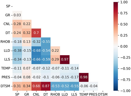
FIGURE 4. Correlation between well logging parameters.

Data is conditioned before training the machine learning model. First, we calibrated the anomalies in the RHOB and DT curves, which are caused by the drilling hole enlargement. Then, we conducted the data normalization to the GR, SP, DT, RHOB, and CNL curves to eliminate the systematic error caused by the differences in logging tools and scales. The JE2 well is chosen as the standard well because of its good logging quality, and the XVa1 is chosen as the standard formation for its consistency in lithology. Finally, the additional features are extracted by the feature engineering technique to further improve the model accuracy. Two numerical features and one categorical feature are introduced, namely, TEMP (Temperature), PRES (Pressure), and FORM (Formation). The TEMP and PRES curves are calculated by the corresponding gradient and measured depth; both parameters are critically related to the fluid properties and also utilized in the rock physics modeling. The categorical feature FORM is the layer information that represents different sets that have distinct lithological and electrical characteristics. The layers are often accurately assigned in wells and can be compared laterally through the whole block. For instance, the XVa1 layer is a pure limestone formation that is evenly distributed across the gas block with a small amount of clay and high porosity. The categorical feature FORM is handled by the feature engineering technique; therefore, it can be applied in machine learning. It is transformed into a numerical feature by One-Hot-Encoding, which replaces the original categorical values with the binary values of 0 and 1 (Figure 5).

FIGURE 5

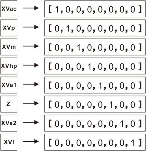
FIGURE 5. Illustration of the data type transformation of FORM by One-Hot-Encoding.

The dataset is divided into three subsets for training, validation, and test purposes. The JE1 and JE2 wells are merged and randomly split into training and validation sets at a ratio of 70% and 30%. The data in the BJE1 well is held for testing and is not involved in the model training and optimization process. The ratio of data instances for training, validation, and testing is 3,126:1734:1042.

4 Methods

4.1 Light Gradient Boosting Machine (LightGBM)

The LightGBM is a gradient boosting framework that is widely used in machine learning competitions and real-world applications. The algorithm is designed to be efficient, scalable, and accurate, and can handle large-scale data and requires less memory than other boosting frameworks. The LightGBM shares a similar objective function as the Extreme Gradient Boosting machine, which introduced a loss function Ω to let the model take a smaller prediction step and prevent overfitting (Chen and Guestrin, 2016; Ke et al., 2017). The objective function for the t_th tree is:

${\mathit{o}\mathit{b}\mathit{j}}^{\mathit{t}}=\left[\sum _{\mathit{i}=\mathbf{1}}^{\mathit{N}}\mathit{L}\left({\mathit{y}}_{\mathit{i}},{\widehat{\mathit{y}}}^{\left(\mathit{t}-\mathbf{1}\right)}+\mathit{P}\right)\right]+\frac{\mathbf{1}}{\mathbf{2}}\mathit{\lambda }{\mathit{P}}^{\mathbf{2}}+\mathit{\gamma }\mathit{T}(1)$

where L is the loss function, N is the total number of samples, y_i is the true value of the ith label, ${\widehat{y}}^{\left(t-1\right)}$ is the predicted value from the previous tree, p is the predicted value of the t_th tree, λ is a penalty hyper parameter for which larger values can shrink the prediction step. γ is another penalty hyperparameter that is used to avoid overfitting by setting a threshold for pruning the branches. T is the total number of nodes in the t_th tree.

The objective is to minimize the loss function to find the lower value for the objective function. The term γT can be omitted as it is a constant. The framework provides a general solution for minimizing any loss function that can be differentiated by approximating the loss function using the second order Taylor polynomial expansion:

$\mathit{L}\left({\mathit{y}}_{\mathit{i}},{\widehat{\mathit{y}}}^{\mathit{t}-\mathbf{1}}+\mathit{P}\right)\approx \mathit{L}\left({\mathit{y}}_{\mathit{i}},{\widehat{\mathit{y}}}^{\mathit{t}-\mathbf{1}}\right)+{\mathit{L}}^{\prime }\left({\mathit{y}}_{\mathit{i}},{\widehat{\mathit{y}}}^{\mathit{t}-\mathbf{1}}\right)\mathit{P}+{\frac{\mathbf{1}}{\mathbf{2}}\mathit{L}}^{″}\left({\mathit{y}}_{\mathit{i}},{\widehat{\mathit{y}}}^{\mathit{t}-\mathbf{1}}\right){\mathit{P}}^{\mathbf{2}}(2)$

where the first and second order derivatives are the gradient and hessian information for the loss function, which are represented by g and h, respectively. The objective function can be written as:

${\mathit{o}\mathit{b}\mathit{j}}^{\mathit{t}}=\frac{\mathbf{1}}{\mathbf{2}}\left(\mathit{H}+\mathit{\lambda }\right){\mathit{P}}^{\mathbf{2}}+\mathit{G}\mathit{P}(3)$

$\mathit{H}=\sum _{\mathit{i}=\mathbf{1}}^{\mathit{N}}{\mathit{h}}_{\mathit{i}}(4)$

$\mathit{G}=\sum _{\mathit{i}=\mathbf{1}}^{\mathit{N}}{\mathit{g}}_{\mathit{i}}(5)$

The optimal predicted value for the t_th tree is when:

$\mathit{P}=-\frac{\mathit{G}}{\mathit{H}+\mathit{\lambda }}(6)$

For the regression task we presented in this study, the loss function is:

$\mathit{L}\left(\mathit{y},\mathit{P}\right)=\frac{\mathbf{1}}{\mathbf{2}}{\left(\mathit{y}-\mathit{P}\right)}^{\mathbf{2}}(7)$

G in (5) becomes the sum of all the residuals in a node, and H in (5) is the number of residuals.

The LightGBM model utilizes different sample selection and a tree building strategy to greatly improve the training speed while maintaining accurate predictions.

4.1.1 Histogram algorithm

To find the best splitting point of a leaf, instead of presorting and traversing each value of every feature to calculate the best gain, the histogram algorithm separates the continuous values into bins and greatly reduces the calculation time.

4.1.2 Gradient-based one-side sampling

The LightGBM uses the gradient-based one-side sampling technique to reduce the sample amount for each training without jeopardizing the model performance. The technique is achieved by calculating the gradient of the loss function of each instance in the training dataset; then, the data with larger gradient gain more weight while the smaller instances are downsampled. It allows the LightGBM to concentrate on the most informative and valuable instances, which increase the training speed and model performance.

4.1.3 Exclusive feature bundling

The exclusive features, by definition, are features that seldom take non-zero values simultaneously. For instance, the one-hot-encoded feature FORM in this study assigned value one only in the corresponding layer. Thus, bundling these exclusive features together can effectively reduce the feature dimensionality to improve efficiency while allowing the model to maintain the predicting performance.

4.1.4 Leaf-wise tree growing

Leaf-wise tree growing is a tree building algorithm utilized by gradient boosting frameworks. Compared with the depth-wise tree growing technique, which is an alternative tree building algorithm, the leaf-wise algorithm builds the tree node-by-node instead of level-by-level. It chooses the largest gain node as the foundation of the next node until the maximum tree depth is reached. The algorithm can capture the complex interaction between features and achieve accurate results with fewer trees, thus resulting in a faster training speed.

4.2 Evaluation metrics

Evaluation of the machine learning model is essential before deployment, and the evaluation methods often vary with the specific tasks. For the regression task in this study, we adopted the root mean squared error (RMSE) and coefficient of determination (R²) to evaluate the fitting and predicting performance of the trained machine learning models. The RMSE is an absolute value that represents the dispersion degree from the true value in a dataset; the lower the RMSE, the better performance of the model prediction. R² indicates the proportion of variance in the predicted value that can be explained by the variance in true value. The model performs well when R² is close to 1. The metrics are expressed as:

$\mathit{R}\mathit{M}\mathit{S}\mathit{E}=\sqrt{\frac{\mathbf{1}}{\mathit{m}}\sum _{\mathit{i}=\mathbf{1}}^{\mathit{m}}{\left({\mathit{y}}_{\mathit{i}}-{\widehat{\mathit{y}}}_{\mathit{i}}\right)}^{\mathbf{2}}}(8)$

${\mathit{R}}^{\mathbf{2}}=\mathbf{1}-\frac{\sum _{\mathit{i}=\mathbf{1}}^{\mathit{m}}{\left({\mathit{y}}_{\mathit{i}}-{\widehat{\mathit{y}}}_{\mathit{i}}\right)}^{\mathbf{2}}}{\sum _{\mathit{i}=\mathbf{1}}^{\mathit{m}}{\left({\mathit{y}}_{\mathit{i}}-{\overline{\mathit{y}}}_{\mathit{i}}\right)}^{\mathbf{2}}}(9)$

where m is the number of data instances, $y_i$ is the measure value, ${\widehat{y}}_i$ is the prediction from the model, and ${\overline{y}}_i$ is the average of prediction. It should be noted that the value of R² could be negative based on the definition (Equation 9), and the negative value occurs when the model fits poorly to the data and makes worse predictions.

4.3 Optuna automatic hyperparameter optimization

Hyperparameter tuning is a crucial step for creating a stable and accurate model. Normally, the step involves manually testing each hyperparameter by grid-search and n-fold cross-validation; the process is considered both time consuming and resource-intensive, and highly affected by experience. Automating the tuning process can greatly expand the searching parameter and the range and improve the model generalization capability. Moreover, it ensures the models are optimized for the task and dataset at hand so it can provide an impartial comparison between different machine learning models.

In this study, we adopt Optuna, an open-source automatic hyperparameter optimization framework (Akiba et al., 2019). The basic workflow of Optuna involves three steps: 1. define the search space for the hyperparameters being optimized and their value ranges; 2. define the objective function and use the validation set for measuring the model performance; and 3. run the optimization algorithm for the search space and find the best value combination for the predefined parameters. The optimized model is then ready for implementation on the test set.

4.4 Shapley Additive Explanations

The Shapley value originated from game theory and was invented by Lloyd Shapley to quantify a player’s contribution in a team (Shapley, 1952; Strumbelj and Kononenko, 2014). Lundberg and Lee (2017) adapted this method to machine learning to explain how each feature contributes to the model outputs. They defined that for a set of features X and simplified features X′, if x≈x', then the model f(x) can approximate the explanatory model g (x’). The explanatory model can be expressed as:

$\mathit{g}\left({\mathit{x}}^{\prime }\right)={\mathit{\phi }}_{\mathbf{0}}+{\displaystyle \sum _{\mathit{i}=\mathbf{1}}^{\mathit{M}}}{\mathit{\phi }}_{\mathit{i}}{{\mathit{x}}_{\mathit{i}}}^{\prime }(10)$

where x_i is the binary version of input feature x, M is the total number of feature inputs, φ₀ is the average output of the model, and φ_i is the Shapley value that measures the contribution of the feature i to the model output, which is expressed as:

${\mathit{\phi }}_{\mathit{i}}={\displaystyle \sum _{\mathit{S}\subseteq \left\{{\mathit{x}}_{\mathbf{1}},\dots ,{\mathit{x}}_{\mathit{M}}\backslash {\mathit{x}}_{\mathit{i}}\right\}}}\frac{\left|\mathit{S}\right|!\left(\mathit{M}-\left|\mathit{S}\right|-\mathbf{1}\right)!}{\mathit{M}!}\left(\mathit{f}\left(\mathit{S}\bigcup \left\{{\mathit{x}}_{\mathit{i}}\right\}\right)-\mathit{f}\left(\mathit{S}\right)\right)(11)$

where S is the combination of all possible subsets of features that excluded x_i.

It has been proven that the Shapley value is satisfied for three properties of the additive feature attribution of the explanatory model: local accuracy, missingness, and consistency.

Local accuracy claims the explanatory model can approximate to the original machine learning model when the simplified feature of x’ approximates input feature x.

$\mathit{f}\left(\mathit{x}\right)\approx \mathit{g}\left({\mathit{x}}^{\prime }\right)\left(\mathbf{f}\mathbf{o}\mathbf{r}\mathbf{x}\approx {\mathbf{x}}^{\prime }\right)(12)$

Missingness defines that the Shapley value should be zero when feature xi’ is missing, i.e., if x’=0, then φ_i=0. For our study, x_i’=1 as all the features in the tabular dataset exist. Consistency shows that if feature x’s contribution changes as the original model changes, then the attribution of the explanatory model should change in the same direction.

In practice, the computation time to calculate the Shapley value for a tree-ensemble can be overwhelming, as indicated by the computational complexity:

$\mathit{O}\left(\mathit{T}\times \mathit{L}\times {\mathbf{2}}^{\mathit{M}}\right)(13)$

where T and L are the maximum number of base learners and leaves in the model, and 2^M is all the possible subsets for M features. Hence, the computational time will increase exponentially for data with numerous features. In our study, an approximation method named TreeSHAP is adopted, which designated for tree structure machine learning models to provide consistent attribute feature importance and greatly accelerate the computational speed (Lundberg and Lee, 2017; Lundberg et al., 2018).

5 Results and comparison

To demonstrate the effectiveness of the TEMP, PRES, and FORM in estimating the shear wave velocity, we built and evaluated four LightGBM models with different feature combinations using the default hyperparameter value (Table 1). The baseline score was calculated using the fivefold cross validation method based on the data from JE1 and JE2. The ‘Full_log plus’ model, which uses the complete seven logging with three additional features, achieved the highest score, with 2.54 for RMSE and 0.93 for R². The lowest score was achieved by the ‘Five_log’ model, which lacks RHOB and CNL loggings parameters. It was shown that the added features in the ‘Five_log plus’ model compensated for the missing logs and improved the ‘Five_log’ model to a score that was close to the ‘Full_log plus’ model. For future use of the model in development wells, the feature combination in ‘Five_log plus’ was chosen for the following hyperparameter tuning and model implementation.

TABLE 1

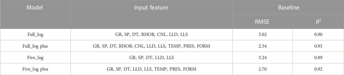
TABLE 1. Model evaluation with different input feature combinations.

Data from JEI and JE2 was randomly split into training (70%) and validation (30%) subsets for the hyperparameter tuning process. The LightGBM hyperparameters that are crucial for the prediction performance were chosen (Table 2). During the tuning practice, we found that the optimal hyperparameter value combinations were often found at approximately 300–700 rounds. Hence, a 1,000 iteration time was set for the tuning process in this study instead of setting an early stopping criterion; therefore, the best model can be built for each machine learning algorithm and equitable comparison between models are possible.

TABLE 2

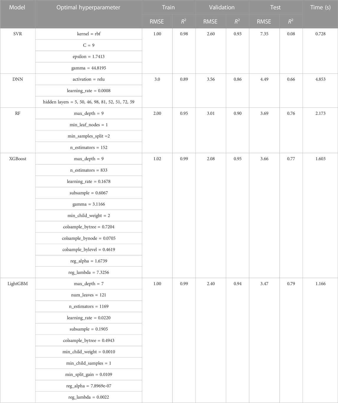
TABLE 2. Optimal hyperparameter values of machine learning models and the evaluation results.

The optimization process using the Optuna package starts from a random combination with an objective value of 3.7; then, after several attempts, the best value soon drops to 2.4. Hyperparameters with different value combinations are tested 1,000 times; during the process the objective value jumps between 2.3 and 4. As the best value tends to stabilize after 20 trials, several subtle drops of values like descending steps can be observed on the red line, which records the best value, at approximate trial positions of 100, 210, and 700 (Figure 6). Finally, the best value of 2.32 is found at trial position 721.

FIGURE 6

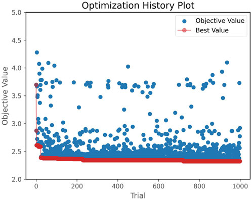
FIGURE 6. Optimization history of the LightGBM model with 1,000 iterations.

The Optuna optimization framework also provides visualization of the tuning process of each individual hyperparameter, which supplements the analysis of the optimization progress. Figure 7 illustrates how the objective value varies during the tuning; the y-axis is the objective value and the x-axis shows the search range for each parameter. Each circle represents a trial; as the trial time increases the color darkens. The figure demonstrates that the trial numbers are sufficient for the search algorithm to fully cover the search range and test for every possible combination. In the first few hundred trials, the algorithm already covers most of the values, and as the number of trials increases, the search range shrinks down to a narrow range and continues to test for the optimal combination. The ‘max_depth’ parameter shows a different pattern than the others because it is set to discrete integer values, whereas others are continuous.

FIGURE 7

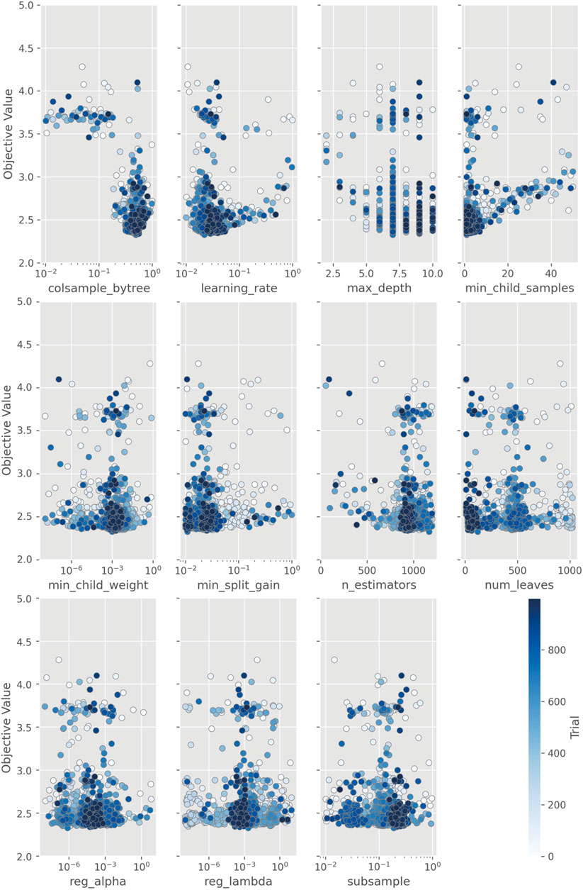
FIGURE 7. The optimization history of each hyperparameter of the LightGBM model.

After each hyperparameter is assigned with the optimal value (Table 2), the LightGBM model is then implemented on the test set, which is the well BJE1. Figure 8 shows predictions for all subsets in which the x-axis is the predicted DTSM value and the y-axis indicates the true DTSM values. It clearly demonstrates that the model has a high accuracy in predicting the shear wave velocity in the study field. The scattered points of all sets are distributed closely to the black dashed diagonal line, indicating that the prediction and true value are nearly the same and have a high degree of correlation. The evaluation metrics of the model are RMSE = 1.0 and R² = 0.99 for the training set, RMSE = 2.40 and R² = 0.94 for the validation set, and RMSE = 3.47 and R² = 0.79 for the test set. The results quantitatively demonstrate that the model is not only well tuned to fit the training data but also has a strong generalization capability to predict shear velocity in other wells.

FIGURE 8

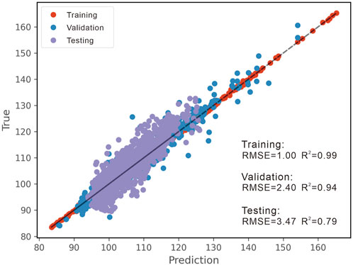
FIGURE 8. The results of the training and implementation of the LightGBM model.

To further demonstrate the accuracy and efficiency of the LightGBM model, four classical supervised machine learning models were introduced and compared with the LightGBM model, namely, Support Vector Regressor (SVR), Deep Neural Network (DNN), Random Forest (RF) and Extreme Gradient Boosting (XGB). Note that RF and XGB are both tree-based models but with different ensemble strategies. All models were trained using the same dataset and tested on the BJE1 and tuned by the Optuna hyperparameter optimization framework.

Table 2 shows the hyperparameters that were used to tune the models and their best value, and Figure 9 demonstrates the prediction results for different subsets. The results show that the tree-based methods overall perform better than the SVR and neural-net based machine learning models. Both RF and XGB had a good performance in fitting the training data and predicting the validation and test data (Table 2). The SVR model has the same accuracy as XGB in fitting the training data, whereas the generalization capability is the worst among all models (RMSE=7.35 and R²=0.08 for the test set by SVR). The scatter plot of the SVR model for the test dataset shows a clear bias from the diagonal line, indicating that the SVR tends to overfit the training data and is insufficient in predicting the shear wave velocity from other wells (Figure 9A). The DNN performs moderately among all on both the validation and test datasets but the generalization capability is stronger than SVR (Figure 9B). The RF showed a more dispersive pattern of the scatter points than XGB (Figures 10C,D).

FIGURE 9

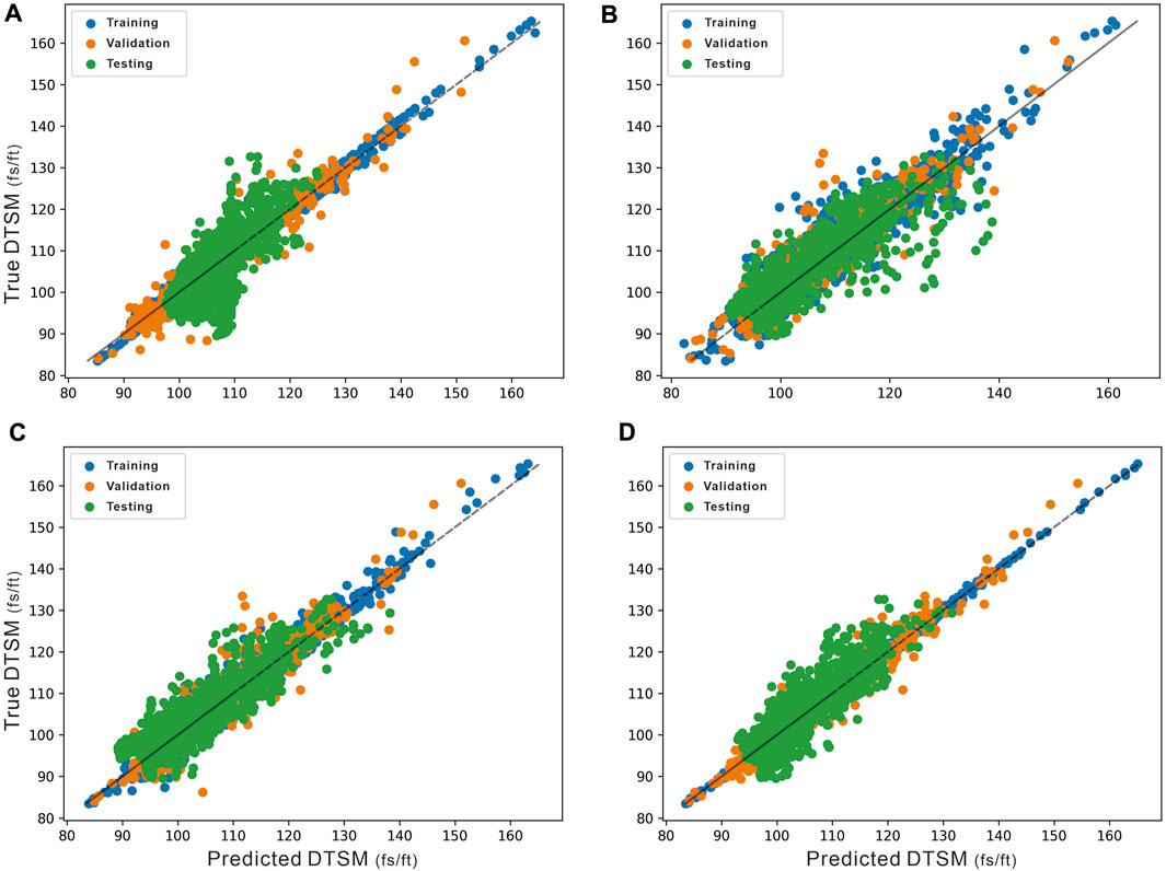
FIGURE 9. Shear velocity predictions from different ML models. (A) SVR. (B) DNN. (C) RF. (D) XGBoost.

FIGURE 10

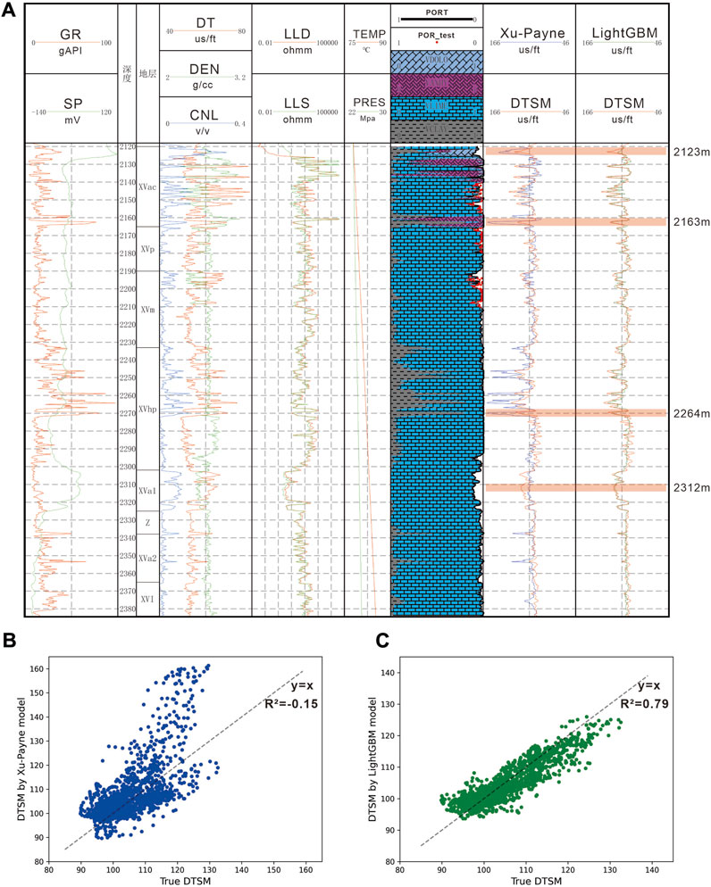
FIGURE 10. Well loggings of BJE1 wells and the comparison between the Xu-Payne model and LightGBM model. (A) Well loggings of BJE1. (B) Crossplot of predictions from the Xu-Payne model versus the true DTSM value. (C) Crossplot of predictions from the LightGBM model versus the true DTSM value.

Training efficiency is another important aspect for model comparison, which has normally been ignored in previous studies. Among the tree-based models, RF spent the most time in the hyperparameter tuning process and costs 2.173 s per training in 1,000 iterations, while XGBoost and LightGBM cost 1.603 s and 1.166 s per training, respectively (Table 2). Time differences are mainly caused by tree assembling strategy. RF uses a bagging strategy, meaning each tree is trained separately with the whole data or a subset of the data. XGBoost and LightGBM use a boosting technique that trains each tree by the residuals from the previous tree and vastly improves the speed. Benefit from the sampling strategy and feature reduction techniques, the LightGBM model is 37% faster than the XGBoost model. As our study only contains three wells, the improvement in training time will be greater when more wells are included.

Another effective approach for the rock elastic property estimation is rock physics modeling. This study employed the Xu-Payne model to calculate the carbonate shear wave velocity in the Callovian-Oxfordian formation and compared it with the prediction from LightGBM model. The modeling process of the Xu-Payne model starts with forming the rock matrix by mixing various mineral components, including limestone, anhydrite, dolomite, and clay content using the Reuss-Voigt-Hill average. Then, pores of different types and shapes are introduced into the matrix according to the Differential Effective Media theory and Kuster–Toksoz theory. The fluid is modeled by considering the reservoir temperature, pressure, water saturation, salinity, and gas-specific gravity. Finally, the rock frame is saturated with the fluid based on the Gassmann theory (Xu and Payne, 2009).

Figure 10A demonstrates the loggings and lithology interpretations that are crucial for the rock physics modeling process. The comparison between the results estimated from the Xu-Payne model (blue curve) and LGBM model (green curve) with original DTSM (red curve) are shown in the last two columns of Figure 10A and in the scatter plots of Figures 10B,C. Evidently, compared with the prediction from LGBM, the Xu-Payne model’s result has a high dispersion degree (RMSE = 8.22) and low accuracy (R² = −0.15). The rock physics model only provides credible results in the XVp and XVm formations, whereas in other formations, the predictions are shifted from the true value, which may be caused by the complex lithology, high clay content, and high porosity. The XVac formation has more lithology types than others as it went through a variation in sedimentary environment; it includes limestone, clay, dolomite, and gypsum. At a depth of 2,123 m, all four lithofacies can be observed, and the Xu-Payne model provides a lower velocity value than the logging. At a depth of 2,163 m in XVac and a depth of 2,264 m in XVhp, the high clay content is the main reason that causes the Xu-Payne model to miscalculate the shear velocity. At a depth of 2,312 m, where limestone is the main lithology type and porosity is approximately 15%, the Xu-Payne model overly estimates the velocity. By contrast, the LGBM model prediction is unaffected by the above factors and predicts the true value accurately.

The prediction error caused by the rock physics model is that the modeling progress relies heavily on the accurate well logging interpretation of petrophysical properties and lithological facies. The interpretation can be strongly biased from the true value without sufficient calibration from the rock sample tests. In our study, only the upper three formations are tested for porosity (Figure 10). Consequently, predictions in the upper three formations are generally more stable than the lower formations. Specifically, the shear velocity at the high porosity area at approximate depths of 2,155 m and 2,195 m is correctly predicted by the Xu-Payne model, whereas the model fails at a depth of 2,312 m where porosity interpretation is not adjusted. However, the machine learning algorithm can skip the well log interpretation procedure and directly establish the non-linear relationship between the loggings and the target value. The following section explains how the output from LightGBM is achieved in detail.

6 Model interpretation

The SHAP analysis is conducted for the LightGBM model trained by five logging parameters and three added features. Both global and individual interpretations are provided for the model. The global interpretation presents an overview and ranking of the contributions of each feature in a quantitative manner, while the individual interpretation dives into a single data instance and demonstrates how each prediction is generated. An explanation of machine learning model is significant for the shear wave velocity regression task, as it can provide valuable insights into the feature selection.

6.1 Global interpretation

Global interpretation from SHAP is first introduced to provide an overview of feature importance. The importance of each input variable is calculated by averaging the absolute Shapley value, which quantitatively represents the general impact of each feature on the model output. Figure 11A displays the sorted mean absolute SHAP value of all the input features in the LightGBM model. It shows that DT has the most significant influence on the model, which consists of the high correlation with DTSM (correlation = 0.87). Additionally, the LLS has a major influence, while its impact on the model is less than half of that as DT. The contribution of the rest features shows a small variation, while the ranking is inconsistent with the correlation in Figure 4. Although the LLD has a higher correlation with DTSM than the SP, the contribution of SP ranks higher; even the TEMP has a greater impact than the LLD. The SP log is used to differentiate the formations with different permeability, which is the result of the interaction between the connected pores and the fine-grained sediments that block the channel. The higher impact of SP on the model may infer that the porosity and lithology significantly contribute to the shear wave velocity of the formation. The added categorical feature FORM ranks behind the LLD and contributes more to the model than the GR. The impact of PRES may be affected by its correlation with TEMP. Despite PRES having the lowest influence on the model output, the importance is as much as 60% of GR.

FIGURE 11

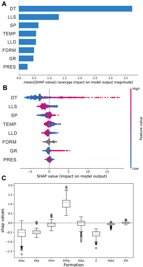
FIGURE 11. Global interpretation of the LightGBM model. (A) SHAP feature importance. (B) SHAP summary plot. (C) SHAP value of the categorical feature FORM.

Figure 11B illustrates the SHAP value distribution of each input variable and the trend of the corresponding feature. The y-axis indicates the input variables in order of importance (same as Figure 11A), and the corresponding SHAP value can be found on the x-axis. Each circle represents a sampling point of the feature, and the color gradient of the variable follows the varying trend from small (blue) to large (red). It should be noted that the negative SHAP value of the feature does not equal to negative influence but to a lower-than-average output from the model. For instance, DT has a wide distribution on the SHAP value where a high DT value has a greater impact on the model and can lead to a higher output, while the low value has a relatively smaller impact and tends to generate lower than average outputs. It can be observed that the LLD and LLS have a reverse trend similar to DT, meaning large resistivity values can lead to small DTSM outputs, agreeing with the negative correlation of these features with the DTSM (Figure 4). Both the SP and GR are used as lithology indicators in well-logging interpretation; the value of the SP is unrelated to the SHAP value, whereas the GR has a trend like DT, indicating that a high gamma value corresponds to a large DTSM output. The TEMP and PRES show a reverse trend similar to the LLD and LLS, which is intuitive as the deeper formation normally has a higher velocity.

The FORM value is discrete and non-numerical; hence, the feature value is colored grey in Figure 11B. The SHAP value of categorical feature FORM is calculated and presented separately in a boxplot, where the formation name is shown on the x-axis and the SHAP value is presented on the y-axis (Figure 11C). It shows that XVhp has the greatest influence on the model, which indicates that the FORM value is most useful in the XVhp layer. Additionally, the XVac, XVp, XVm, XVa1, and Z layers make a positive contribution to the model but are less influential. The lowest two layers XVa2 and XVI hardly make any contribution.

6.2 Local interpretation

Local interpretation by SHAP is provided for individual data instances to examine the contribution and the interaction between the input variables. Four predictions at various depths that represent different reservoir characteristics were chosen for the local interpretation. The individual predictions are at depths of 2,123 m, 2,163 m, 2,264 m, and 2,312 m, which correspond to the places where LightGBM outperforms the rock physics model in Figure 10. The value of each feature is shown on the y-axis, and the x-axis is the prediction. The E [f(X)] is the base value, which is the mean value of the DTSM in the validation subset. The final prediction expressed by f(x) is the summation of the contributions from all the features plus the base value.

A depth of 2,123 m in the XVac layer represents a reservoir condition where four lithofacies co-exist (Figure 12A). Here, the GR=39.965 and contributes the most to the LightGBM model given by the SHAP value of +3.97, followed by LLS=0.815 and LLD=−0.857, for which the SHAP values are +1.98 and +1.38, respectively. The absolute SHAP value for the rest features is smaller than 1. The added feature FORM=XVac and PRES=23.529 has greater significance than DT=55.01, for which the SHAP value is −0.6. The summation of all the features drives the base value toward the final prediction (112.14 us/ft), which is close to the true value (125.161 us/ft).

FIGURE 12

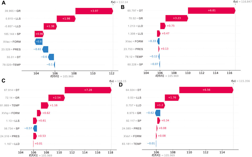
FIGURE 12. Individual interpretation for data instances at various depths. (A) 2,123 m. (B) 2,163 m. (C) 2,264 m. (D) 2,312 m.

Figures 12B,C display the data at depths of 2163 m and 2264 m, where the rock physics model tends to overestimate the DTSM value. Both places have a high clay content (GR>70), and the LightGBM model chose DT=65.797 as the dominating feature, which contributes twice as much as GR=70.52. The other features have a relatively small impact on the model but still manage to influence the precision of the output. The final predictions for both places (116.847 us/ft and 118.15 us/ft) are close to the DTSM logging value (117.640 us/ft and 129.102 us/ft).

Figure 12D demonstrates a typical high porosity region at a depth of 2312 m, where the rock physics model failed to provide an accurate result. The feature DT=64.024 continues to dominate the ranking in feature importance. The contribution of the rest logging features follows the ranking of correlation with DTSM (Figure 4), and the added features have the smallest impacts. The final prediction (115.356) is also close to the measure value (116.262 us/ft).

The individual interpretations demonstrate that the LightGBM model can adapt to different reservoir conditions and provide accurate and stable estimations of the target value. Moreover, the results indicate that the importance of each feature does not necessarily correspond to its linear correlation with DTSM. It is also worth noting that the contribution of each feature varies with data instances, and it does not strictly coincide with the ranking in global interpretation. For instance, DT has the greatest general impact on the model while it contributes less than FORM and PRES at a depth of 2123 m (Figure 12A); the correlation between LLD and DTSM is 0.50, while its importance ranks the lowest among all features at a depth of 2264 m (Figure 12C). The result shows that each feature in the model has a positive influence on the final output. The newly added features are proven to be useful to the prediction and can effectively compensate for the decrease in model accuracy caused by the absence of RHOB and CNL.

In addition to the evaluation metric from testing the model on a test well, the SHAP analysis offers another approach for verifying the reliability and effectiveness of a model by checking whether the feature dependency with the target value conforms to the geological background. Figure 13 displays the dependency plot of each feature, with the x-axis showing the feature value and y-axis representing the SHAP value. Each plot is colored with a feature that has the largest interaction effect.

FIGURE 13

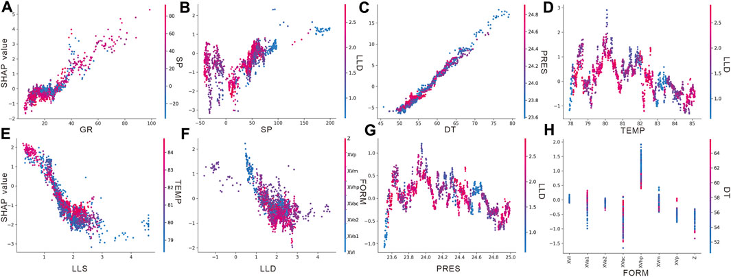
FIGURE 13. Dependency plot of input variables for the LightGBM model. (A) GR. (B) SP. (C) DT. (D) TEMP. (E) LLS. (F) LLD. (G) PRES. (H) FORM.

The result shows that the increasing value of DT, SP, and GR leads to the elevation of their SHAP value, which corresponds with their positive relationship with DTSM. It is clear that DT has the best correlation with DTSM, and its interaction with PRES indicates the formation at a greater depth, which has a larger PRES value and tends to have a greater velocity; the GR and SP logs are normally used to calculate the shale volume, and larger values mean a greater clay content. In Figures 13A,B, the large values of the GR and SP lead to an increase in DTSM values, which agrees with the fact that a greater clay content can cause a drop in Vs velocity. Additionally, the SP log performs worse than the GR in calculating the shale volume in a carbonate formation; hence, the correlation trend in SP is not as clear as in the GR. The increase in SHAP is followed by decreasing LLD, LLS, TEMP, and PRES values, indicating that the features are negatively correlated with the DTSM. The negative trend of LLD and LLS with DTSM agrees with the fact that Vs decreases with the increasing gas saturation, as the gas bearing formation can cause larger resistivity than the water bearing formation. The negative trend of TEMP and PRES is also rational, as both features are directly related to depth and the deeper formation tends to have a larger velocity caused by mechanical and chemical compaction. The results correspond well with the complex carbonate reservoir condition in most layers. It corresponds with the complex carbonate reservoir condition in most layers, e.g., XVac has the most complex lithofacies, XVam and XVa1 have high porosity, and the XVhp layer has a high clay volume; XVI and XVa2 are interpreted as pure limestone formations with a small amount of clay and pore volume. The result indicates that the categorical feature FORM can be helpful to the machine learning model, especially for the complex carbonate formations.

7 Conclusion

Machine learning methods have been prevalently utilized in the well-logging estimation of shear wave velocity. However, owing to the black-box nature of the machine learning model, most research emphasizes the effectiveness of new algorithms, and the input features are limited to the traditional logging parameters. This study adopts the LightGBM model to estimate the shear wave velocity in a complex carbonate formation. To expand the usability of the model in development wells that normally lack essential loggings, we introduced three new features into the model, including two numerical features (temperature and pressure) and one categorical feature (formation). The model is best tuned with the automatic hyperparameter optimization framework Optuna, and the result is compared with four regression machine learning models that were optimized with the same process. The Xu-Payne rock physics model is also applied for calculating the Vs and compared with the LightGBM model. Furthermore, we use the Shapley Additive Explanations (SHAP) to interpret the LightGBM model and quantitatively demonstrate the contribution of each feature and validate the reliability of the trained model.

The following conclusions can be drawn from this study.

1. The newly added features are proved effective prior to the application of the model. Four combinations of different features are tested using the LightGBM model with default hyperparameters. Both RMSE and R² are decreased with the absence of RHOB and CNL log, while adding the new features can compensate the loss of important logs and improve the model performance.

2. The application of the automatic hyperparameter optimization framework is essential and can provide a fair comparison between different machine learning algorithms. As the hyperparameter tuning is crucial for building a model, the artificial tuning process that normally involves grid-search and k-fold cross validation can be inaccurate and time consuming. Utilizing the Optuna framework can greatly expand the searching area and guarantee a stable result, which ensures the equitable comparison between different machine learning models.

3. The LightGBM model outperforms the other machine learning models in both accuracy and efficiency. The comparison between different models shows the tree-ensemble-based methods perform better than SVR and DNN, and the LightGBM outperforms other tree-ensemble methods, such as RF and XGBoost. Other than SVR, which shows little generalization capability, the LightGBM has the shortest training time. Additionally, time efficiency is a significant factor to be considered for model selection, as numerous wells could be included when performing the Vs estimation at a larger scale.

4. The LightGBM model performs better than the rock physics modeling approach. The construction of the rock physics model requires the accurate interpretation of petrophysical parameters and lithofacies, while the condition is often unsatisfied without sufficient laboratory tests of rock samples. The LightGBM model can directly establish the non-linear relationship between input variables and Vs without performing the intermediate interpretation step. Thus, the model can generate more accurate results, especially in regions with complex lithofacies, a high clay content, and a high porosity.

5. The importance of input features is not necessarily related to their relationship with Vs The global interpretation provided by the SHAP analysis indicates that the ranking of the contributions of each feature is unrelated to their correlation with Vs, except for DT and LLS. The individual interpretation at different depths further proves that the contribution of each feature varies with their values and the reservoir condition. Moreover, the newly added features can impact the model more than traditional logging parameters, such as LLD and GR.

6. The quantitative interpretation of the model also provides additional evidence on the applicability and effectiveness of the LightGBM model. The dependency between the input features and the SHAP value and the deduced results correspond well with the geological understanding of the target carbonate formation, greatly improving confidence in the further application of machine learning models for shear wave estimation.

Data availability statement

The data analyzed in this study is subject to the following licenses/restrictions: The data is confidetial for commerical purposes. Requests to access these datasets should be directed to zhangtianze@petrochina.com.cn.

Author contributions

Manuscript writing: TZ Programming: TZ and TG Review: LZ and WZ Supervision and validation: HC and HW. All authors contributed to the article and approved the submitted version.

Funding

This research was supported by the Sichuan Science and Technology Program (Grant No. 2022NSFSC0187).

Acknowledgments

The authors thank SK and TZ who provided valuable comments that greatly improved the manuscript.

Conflict of interest

Authors TZ, HW, TG, LZ, and WZ were employed by China National Petroleum Corporation. Author HC was employed by China National Petroleum Corporation International Ltd.

Publisher’s note

All claims expressed in this article are solely those of the authors and do not necessarily represent those of their affiliated organizations, or those of the publisher, the editors and the reviewers. Any product that may be evaluated in this article, or claim that may be made by its manufacturer, is not guaranteed or endorsed by the publisher.

References

Alameedy, U., Alhaleem, A. A., Isah, A., Al-Yaseri, A., El-Husseiny, A., and Mahmoud, M. (2022). Predicting dynamic shear wave slowness from well logs using machine learning methods in the Mishrif Reservoir, Iraq. J. Appl. Geophys. 205, 104760. doi:10.1016/j.jappgeo.2022.104760

CrossRef Full Text | Google Scholar

Alkinani, H. H., Al-Hameedi, A. T., Dunn-Norman, S., Flori, R. E., Al-Alwani, M. A., and Mutar, R. A. (2019). Intelligent data-driven analytics to predict shear wave velocity in carbonate formations: comparison between recurrent and conventional neural networks. New York City: U.S. Rock Mechanics/Geomechanics Symposium. ARMA-2019-0511.

Google Scholar

Akiba, T., Sano, S., Yanase, T., Ohta, T., and Koyama, M. (2005). “Optuna: A next-generation hyperparameter optimization framework,” In Proceedings of the 25th ACM SIGKDD international conference on knowledge discovery and data mining, 2623–2631. doi:10.1145/3292500.3330701

CrossRef Full Text | Google Scholar

Altmann, A., Toloşi, L., Sander, O., and Lengauer, T. (2010). Permutation importance: a corrected feature importance measure. Bioinformatics 26, 1340–1347. doi:10.1093/bioinformatics/btq134

PubMed Abstract | CrossRef Full Text | Google Scholar

Anemangely, M., Ramezanzadeh, A., Amiri, H., and Hoseinpour, S.-A. (2019). Machine learning technique for the prediction of shear wave velocity using petrophysical logs. J. Pet. Sci. Eng. 174, 306–327. doi:10.1016/j.petrol.2018.11.032

CrossRef Full Text | Google Scholar

Anemangely, M., Ramezanzadeh, A., and Tokhmechi, B. (2017). Shear wave travel time estimation from petrophysical logs using ANFIS-PSO algorithm: a case study from Ab-Teymour Oilfield. J. Nat. Gas. Sci. Eng. 38, 373–387. doi:10.1016/j.jngse.2017.01.003

CrossRef Full Text | Google Scholar

Anselmetti, F. S., and Eberli, G. P. (1993). Controls on sonic velocity in carbonates. Pure Appl. Geophys. 141, 287–323. doi:10.1007/BF00998333

CrossRef Full Text | Google Scholar

Azadpour, M., Saberi, M. R., Javaherian, A., and Shabani, M. (2020). Rock physics model-based prediction of shear wave velocity utilizing machine learning technique for a carbonate reservoir, southwest Iran. J. Pet. Sci. Eng. 195, 107864. doi:10.1016/j.petrol.2020.107864

CrossRef Full Text | Google Scholar

Bagheripour, P., Gholami, A., Asoodeh, M., and Vaezzadeh-Asadi, M. (2015). Support vector regression based determination of shear wave velocity. J. Pet. Sci. Eng. 125, 95–99. doi:10.1016/j.petrol.2014.11.025

CrossRef Full Text | Google Scholar

Belle, V., and Papantonis, I. (2021). Principles and practice of explainable machine learning. Front. Big Data 39, 688969. doi:10.3389/fdata.2021.688969

CrossRef Full Text | Google Scholar

Castagna, J. P., Batzle, M. L., and Eastwood, R. L. (1985). Relationships between compressional-wave and shear-wave velocities in clastic silicate rocks. Geophysics 50, 571–581. doi:10.1190/1.1441933

CrossRef Full Text | Google Scholar

Chen, T., and Guestrin, C. (2016). “A scalable tree boosting system,” In Proceedings of the 22nd ACM SIGKDD international conference on knowledge discovery and data mining, 785–794. doi:10.1145/2939672.2939785

CrossRef Full Text | Google Scholar

Dikshit, A., Pradhan, B., and Alamri, A. M. (2021). Pathways and challenges of the application of artificial intelligence to geohazards modelling. Gondwana Res. 100, 290–301. doi:10.1016/j.gr.2020.08.007

CrossRef Full Text | Google Scholar

Du, M., Liu, N., and Hu, X. (2019). Techniques for interpretable machine learning. Commun. ACM 63, 68–77. doi:10.1145/3359786

CrossRef Full Text | Google Scholar

Dvorkin, J. P. (2008). Yet another V S equation. Geophysics 73, E35–E39. doi:10.1190/1.2820604

CrossRef Full Text | Google Scholar

Ebrahimi, A., Izadpanahi, A., Ebrahimi, P., and Ranjbar, A. (2022). Estimation of shear wave velocity in an Iranian oil reservoir using machine learning methods. J. Pet. Sci. Eng. 16, 109841. doi:10.1016/j.petrol.2021.109841

CrossRef Full Text | Google Scholar

Esterhuizen, J. A., Goldsmith, B. R., and Linic, S. (2022). Interpretable machine learning for knowledge generation in heterogeneous catalysis. Nat. Catal. 5, 175–184. doi:10.1038/s41929-022-00744-z

CrossRef Full Text | Google Scholar

Feng, D.-C., Wang, W.-J., Mangalathu, S., and Taciroglu, E. (2021). Interpretable XGBoost-SHAP machine-learning model for shear strength prediction of squat RC walls. J. Struct. Eng. 147, 04021173. doi:10.1061/(ASCE)ST.1943-541X.0003115

CrossRef Full Text | Google Scholar

Garia, S., Pal, A. K., Ravi, K., and Nair, A. M. (2019). A comprehensive analysis on the relationships between elastic wave velocities and petrophysical properties of sedimentary rocks based on laboratory measurements. J. Pet. Explor. Prod. Technol. 9, 1869–1881. doi:10.1007/s13202-019-0675-0

CrossRef Full Text | Google Scholar

Greenberg, M., and Castagna, J. (1992). Shear-wave velocity estimation in porous rocks: theoretical formulation, preliminary verification and applications1. Geophys. Prospect. 40, 195–209. doi:10.1111/j.1365-2478.1992.tb00371.x

CrossRef Full Text | Google Scholar

Hadi, F. A., and Nygaard, R. (2018). Shear wave prediction in carbonate reservoirs: can artificial neural network outperform regression analysis? Seattle, Washington: U.S. Rock Mechanics/Geomechanics Symposium. ARMA-2018-905.

Google Scholar

Han, D., Nur, A., and Morgan, D. (1986). Effects of porosity and clay content on wave velocities in sandstones. Geophysics 51, 2093–2107. doi:10.1190/1.1442062

CrossRef Full Text | Google Scholar

Kittridge, M. G. (2015). Investigating the influence of mineralogy and pore shape on the velocity of carbonate rocks: insights from extant global data sets. Interpretation 3, SA15–SA31. doi:10.1190/INT-2014-0054.1

CrossRef Full Text | Google Scholar

Liu, Y. A., Yang, H. A., Liu, Y. A., Zhu, W. A., and Bie, Q. B. (2013). Characteristics and main controlling factors of the Oxfordian biohermal reservoirs in Girsan of Amu Darya Right Bank, Turkmenistan. Natural Gas Industry 33 (3), 10–14. doi:10.3787/j.issn.1000-0976.2013.03.003

CrossRef Full Text | Google Scholar

Lundberg, S. M., Erion, G. G., and Lee, S.-I. (2018). Consistent individualized feature attribution for tree ensembles. ArXiv Prepr. ArXiv180203888. Available at: https://doi.org/10.48550/arXiv.1802.03888.

Google Scholar

Lundberg, S. M., and Lee, S.-I. (2017). Consistent feature attribution for tree ensembles. ArXiv Prepr. ArXiv170606060. Available at: https://doi.org/10.48550/arXiv.1706.06060.

Google Scholar

Ma, J., Xia, D., Wang, Y., Niu, X., Jiang, S., Liu, Z., et al. (2022). A comprehensive comparison among metaheuristics (MHs) for geohazard modeling using machine learning: insights from a case study of landslide displacement prediction. Eng. Appl. Artif. Intell. 114, 105150. doi:10.1016/j.engappai.2022.105150

CrossRef Full Text | Google Scholar

Mehrad, M., Ramezanzadeh, A., Bajolvand, M., and Reza Hajsaeedi, M. (2022). Estimating shear wave velocity in carbonate reservoirs from petrophysical logs using intelligent algorithms. J. Pet. Sci. Eng. 212, 110254. doi:10.1016/j.petrol.2022.110254

CrossRef Full Text | Google Scholar

Mehrgini, B., Izadi, H., and Memarian, H. (2019). Shear wave velocity prediction using Elman artificial neural network. Carbonates Evaporites 34, 1281–1291. doi:10.1007/s13146-017-0406-x

CrossRef Full Text | Google Scholar

Miah, M. I. (2021). Improved prediction of shear wave velocity for clastic sedimentary rocks using hybrid model with core data. J. Rock Mech. Geotech. Eng. 13, 1466–1477. doi:10.1016/j.jrmge.2021.06.014

CrossRef Full Text | Google Scholar

Molnar, C., Casalicchio, G., and Bischl, B. (2021). “Interpretable machine learning–a brief history, state-of-the-art and challenges,” in ECML PKDD 2020 workshops: workshops of the European conference on machine learning and knowledge discovery in databases (ECML PKDD 2020): SoGood 2020, PDFL 2020, MLCS 2020, NFMCP 2020, DINA 2020, EDML 2020, XKDD 2020 and INRA 2020, ghent, Belgium, september 14–18, 2020, proceedings (Cham: Springer), 417–431.

CrossRef Full Text | Google Scholar

Murdoch, W. J., Singh, C., Kumbier, K., Abbasi-Asl, R., and Yu, B. (2019). Interpretable machine learning: definitions, methods, and applications. ArXiv Prepr. ArXiv190104592. Available at: https://doi.org/10.48550/arXiv.1901.04592.

Google Scholar

Nelder, J. A., and Wedderburn, R. W. (1972). Generalized linear models. J. R. Stat. Soc. Ser. Gen. 135, 370–384. doi:10.2307/2344614

CrossRef Full Text | Google Scholar

Nourafkan, A., and Kadkhodaie-Ilkhchi, A. (2015). Shear wave velocity estimation from conventional well log data by using a hybrid ant colony–fuzzy inference system: a case study from Cheshmeh–Khosh oilfield. J. Pet. Sci. Eng. 127, 459–468. doi:10.1016/j.petrol.2015.02.001

CrossRef Full Text | Google Scholar

Olayiwola, T., and Sanuade, O. A. (2021). A data-driven approach to predict compressional and shear wave velocities in reservoir rocks. Petroleum 7, 199–208. doi:10.1016/j.petlm.2020.07.008

CrossRef Full Text | Google Scholar

Parvizi, S., Kharrat, R., Asef, M. R., Jahangiry, B., and Hashemi, A. (2015). Prediction of the shear wave velocity from compressional wave velocity for Gachsaran Formation. Acta geophys. 63, 1231–1243. doi:10.1515/acgeo-2015-0048

CrossRef Full Text | Google Scholar

Qabany, A. A., Mortensen, B., Martinez, B., Soga, K., and DeJong, J. (2011). Microbial carbonate precipitation: correlation of S-wave velocity with calcite precipitation. Dallas: Geo-Frontiers 2011: Advances in Geotechnical Engineering, 3993–4001.

Google Scholar

Rafavich, F., Kendall, C. S. C., and Todd, T. (1984). The relationship between acoustic properties and the petrographic character of carbonate rocks. Geophysics 49, 1622–1636. doi:10.1190/1.1441570

CrossRef Full Text | Google Scholar

Rajabi, M., Hazbeh, O., Davoodi, S., Wood, D. A., Tehrani, P. S., Ghorbani, H., et al. (2022). Predicting shear wave velocity from conventional well logs with deep and hybrid machine learning algorithms. J. Pet. Explor. Prod. Technol. 13, 19–42. doi:10.1007/s13202-022-01531-z

CrossRef Full Text | Google Scholar

Rezaee, M. R., Ilkhchi, A. K., and Barabadi, A. (2007). Prediction of shear wave velocity from petrophysical data utilizing intelligent systems: an example from a sandstone reservoir of Carnarvon Basin, Australia. J. Pet. Sci. Eng. 55, 201–212. doi:10.1016/j.petrol.2006.08.008

CrossRef Full Text | Google Scholar

Roscher, R., Bohn, B., Duarte, M. F., and Garcke, J. (2020). Explainable machine learning for scientific insights and discoveries. Ieee Access 8, 42200–42216. doi:10.1109/ACCESS.2020.2976199

CrossRef Full Text | Google Scholar

Rudin, C., Chen, C., Chen, Z., Huang, H., Semenova, L., and Zhong, C. (2022). Interpretable machine learning: fundamental principles and 10 grand challenges. Stat. Surv. 16, 1–85. doi:10.1214/21-ss133

CrossRef Full Text | Google Scholar

Seifi, H., Tokhmechi, B., and Moradzadeh, A. (2020). Improved estimation of shear-wave velocity by ordered weighted averaging of rock physics models in a carbonate reservoir. Nat. Resour. Res. 29, 2599–2617. doi:10.1007/s11053-019-09590-6

CrossRef Full Text | Google Scholar

Shan, Y., Chai, H., Wang, H., Zhang, L., Su, P., Kong, X., et al. (2022). Origin and Characteristics of the Crude Oils and Condensates in the Callovian-Oxfordian Carbonate Reservoirs of the Amu Darya Right Bank Block, Turkmenistan. Lithosphere 2022 (1). doi:10.2113/2022/5446117

CrossRef Full Text | Google Scholar

Strumbelj, E., and Kononenko, I. (2014). Explaining prediction models and individual predictions with feature contributions. Knowl Inf Syst 41, 647–665. doi:10.1007/s10115-013-0679-x

CrossRef Full Text | Google Scholar

Sun, S. Z., Wang, H., Liu, Z., Li, Y., Zhou, X., and Wang, Z. (2012). The theory and application of DEM-Gassmann rock physics model for complex carbonate reservoirs. Lead. Edge 31, 152–158. doi:10.1190/1.3686912

CrossRef Full Text | Google Scholar

Taheri, A., Makarian, E., Manaman, N. S., Ju, H., Kim, T.-H., Geem, Z. W., et al. (2022). A fully-self-adaptive harmony search GMDH-type neural network algorithm to estimate shear-wave velocity in porous Media. Appl. Sci. 12, 6339. doi:10.3390/app12136339

CrossRef Full Text | Google Scholar

Tamunobereton-Ari, I., Omubo-Pepple, V., and Uko, E. (2010). The influence of lithology and depth on acoustic velocities in South-east. Am. J. Sci. Ind. Res. 1, 279–292. doi:10.5251/ajsir.2010.1.2.279.292

CrossRef Full Text | Google Scholar

Tian, Y., Xu, H., Zhang, X., Wang, H., Guo, T., Zhang, L., et al. (2016). Multi-resolution graph-based clustering analysis for lithofacies identification from well log data: Case study of intraplatform bank gas fields, Amu Darya Basin. Appl. Geophys. 13, 598–607. doi:10.1007/s11770-016-0588-3

CrossRef Full Text | Google Scholar

Wu, C., Yu, B., Wang, H., Cheng, C., Ruan, Z., Guo, T., et al. (2019). High-resolution sequence divisions and stratigraphic models of the Amu Darya right bank. Arab. J. Geosci. 12, 1–16. doi:10.1007/s12517-019-4416-y

CrossRef Full Text | Google Scholar

Vellido, A. (2020). The importance of interpretability and visualization in machine learning for applications in medicine and health care. Neural comput. Appl. 32, 18069–18083. doi:10.1007/s00521-019-04051-w

CrossRef Full Text | Google Scholar

Wang, H., Sun, S. Z., Yang, H., Gao, H., Xiao, Y., and Hu, H. (2011). The influence of pore structure on P-& S-wave velocities in complex carbonate reservoirs with secondary storage space. Pet. Sci. 8, 394–405. doi:10.1007/s12182-011-0157-6

CrossRef Full Text | Google Scholar

Wang, J., Cao, J., and Yuan, S. (2020). Shear wave velocity prediction based on adaptive particle swarm optimization optimized recurrent neural network. J. Pet. Sci. Eng. 194, 107466. doi:10.1016/j.petrol.2020.107466

CrossRef Full Text | Google Scholar

Wu, C., Cheng, C., Zhang, L., Yu, B., and Wang, H. (2022). Callovian-Oxfordian sedimentary microfacies in the middle of Block B on the right bank of the Amu Darya Basin, Turkmenistan. Energy Geosci., 100136. doi:10.1016/j.engeos.2022.09.006

CrossRef Full Text | Google Scholar

Xing, Y., Wang, H., Zhang, L., Cheng, M., Shi, H., Guo, C., et al. (2022). Depositional and Diagenetic Controls on Reservoir Quality of Callovian-Oxfordian Stage on the Right Bank of Amu Darya. Energies 15 (19), 6923. doi:10.3390/en15196923

CrossRef Full Text | Google Scholar

Xu, S., and Payne, M. A. (2009). Modeling elastic properties in carbonate rocks. Lead. Edge 28, 66–74. doi:10.1190/1.3064148

CrossRef Full Text | Google Scholar

Zhang, G.-Z., Chen, H.-Z., Wang, Q., and Yin, X.-Y. (2013). Estimation of S-wave velocity and anisotropic parameters using fractured carbonate rock physics model. Chin. J. Geophys. 56, 1707–1715. doi:10.6038/cjg20130528

CrossRef Full Text | Google Scholar

Zhang, Y., Zhang, C., Ma, Q., Zhang, X., and Zhou, H. (2022). Automatic prediction of shear wave velocity using convolutional neural networks for different reservoirs in Ordos Basin. J. Pet. Sci. Eng. 208, 109252. doi:10.1016/j.petrol.2021.109252

CrossRef Full Text | Google Scholar

Zhang, Y., Zhong, H.-R., Wu, Z.-Y., Zhou, H., and Ma, Q.-Y. (2020). Improvement of petrophysical workflow for shear wave velocity prediction based on machine learning methods for complex carbonate reservoirs. J. Pet. Sci. Eng. 192, 107234. doi:10.1016/j.petrol.2020.107234

CrossRef Full Text | Google Scholar

Zhong, C., Geng, F., Zhang, X., Zhang, Z., Wu, Z., and Jiang, Y. (2021). “Shear wave velocity prediction of carbonate reservoirs based on CatBoost,” in 2021 4th International Conference on Artificial Intelligence and Big Data (ICAIBD), Chengdu, China, 28-31 May 2021, 622–626. doi:10.1109/ICAIBD51990.2021.9459061

CrossRef Full Text | Google Scholar