Linear site-response characteristics at central and eastern U.S. seismic stations

Abstract
Earthquake S waves can become trapped, or resonate, between the free surface and high-impedance basal layers, strongly contributing to site response at specific frequencies. Strong S-wave resonances have been observed in the central and eastern U.S., where many sites sit on unlithified sediments underlain by stiff bedrock. To evaluate S-wave resonances in this region, we calculated 1D linear site-responses at 89 seismic stations with developed S-wave velocity profiles into bedrock. We found that S-wave resonances at the fundamental and strongest (peak) modes occur across large ranges of frequencies, each spanning more than two orders of magnitude — 0.21–54.0 Hz and 0.29–71.5 Hz, respectively. Amplifications of ∼5 and ∼6 are common at the fundamental frequency and peak modes, respectively; the largest amplification calculated was 13.2. Using simple regression analyses, we evaluated the skills of six proxies derived from the S-wave velocity profiles to predict the frequencies and corresponding amplifications of the fundamental and peak modes. We found that the depths to the 1.0 km/s and 2.5 km/s horizons, consistent with other studies, and to the maximum impedance contrasts strongly correlate with the resonance frequencies and that the fundamental-mode and peak amplifications correlate with the maximum impedance ratios. Correlations improved for data subsets based on the number and magnitude of impedance ratios underlying the sites and are the strongest at sites underlain by a single impedance ratio of 3.0 or greater. Finally, we calculated the S-wave horizontal-to-vertical spectral ratios (HVSR) at each possible seismic station and found, consistent with other studies, that the first peak can be used to estimate fundamental-mode frequencies and the corresponding amplifications. Thus, S-wave HVSR, can provide useful estimates of the fundamental-mode linear site response parameters at sites lacking S-wave velocity profiles. Furthermore, S-wave HVSR curves appear to be useful to broadly categorize impedance-ratio profiles.

1 Introduction

Near-surface geologic layers affect seismic waves. Of particular relevance to people and the built environment are the amplification effects on S-waves caused by the decreasing seismic impedance encountered by the waves as they approach the surface. S-wave amplification can be substantially increased at sites with underlying strong impedance contrasts as the waves become to some degree or another trapped between the free surface and the interface corresponding to the strong contrast, thus resulting in resonance. Three-dimensional structure can result in yet additional amplification due to focusing effects or induced surface waves (e.g., Kawase, 1996). A case of extensive damage due to site resonance occurred in Mexico City, which sits on very soft lake sediments, during the 1985 Michoacan earthquake of magnitude (M) 8.1) (Seed et al., 1988; Singh et al., 1988). Mexico City experienced damaging shaking again during the 2017 Puebla-Morelos Earthquake (M 7.1) (Çelebi et al., 2018). Damage caused by site response has been observed throughout the world during moderate to strong earthquakes (Borcherdt and Glassmoyer, 1992; Hartzell et al., 1996; Woolery et al., 2008; Lu et al., 2010; Asimaki et al., 2017).

To predict earthquake ground-motion hazards most accurately, seismic hazard assessments must account for these site effects—commonly called site response. As the phenomenon’s name implies, site response characteristics are specific to individual sites and the characteristics can vary over short—e.g., 10¹–10² m—distance scales (e.g., Vernon et al., 1991; Thompson et al., 2009; Hallal and Cox, 2021). Thus, site response depends on the local geology and the possibility of subsurface property variations over short distances warrants at best the cautionary use of regional or global site-response characterizations.

Site response has been estimated empirically by the ratio of S-wave amplitude spectra recorded at the site of interest to those at a reference site (Borcherdt, 1970) and using surface-to-bedrock borehole spectral ratios (e.g., Bonilla et al., 2002). Also, the single-station approach, which involves estimating site-response from S waves recorded on the horizontal component and on the vertical component at a single site, has been used with success in some locations (e.g., Lermo and Chávez-García, 1993). Use of this technique, popularized by Nakamura (1989) who used recordings of microtremors, involves calculating the ratio of horizontal-to vertical-component amplitude spectra (HVSR) and assumes the vertical-component approximates reference-site horizontal ground motions.

Because site response is the result of 3D wave propagation phenomena in the upper crust and near-surface layers, the preferred theoretical approach to quantify site response involves 3D ground-motion modeling (e.g., Rodgers et al., 2020). However, application of such modeling for site response estimation is limited by the resolution of the earth model, nonlinearity, and computational restrictions at high frequencies. Thus, although higher-resolution models appropriate for such applications are being developed, (e.g., Panzera et al., 2022), current practice typically uses 1D theoretical approaches to model site response (e.g., Harmon et al., 2019) including linear matrix propagation method (Haskell, 1953; 1960), ray-theory-based linear square-root impedance (Boore, 2003), equivalent linear (e.g., STRATA; Kottke and Rathje, 2008), and nonlinear methods (e.g., DEEPSOIL; Hashash et al., 2015). The matrix propagation method has been the most widely used to calculate 1D linear and equivalent linear SH-wave amplification functions for profiles of S-wave velocity (Vs) and other dynamic parameters.

Both the empirical site response amplification functions and those derived by 1D modeling are frequency dependent. For example, the borehole transfer function, S-wave HVSR, and 1D theoretical transfer function from the CUSSO vertical seismic array (Woolery et al., 2016), upper Mississippi Embayment, shown in Figure 1 all have peaks and troughs. These peaks and troughs, which correspond with SH-wave resonance modes (Boore, 2013), demonstrate that S-wave resonance controls the site response at this site, although the peaks are manifested slightly differently in the various spectral ratios. The strong frequency dependence is not accounted for in simple ray theory where the amplification of an ascending seismic ray is proportional to the square root of the ratio of the impedance at a ray’s reference point to that at the receiver’s location (Aki and Richards, 1980; Boore, 2003). Although the close correspondence between the empirical and 1D spectral ratios observed at CUSSO does not occur at all global borehole sites (Thompson et al., 2012; Pilz and Cotton, 2019), numerous studies have shown such correspondences exist broadly at sites with accurate soil models (e.g., Wang and Carpenter, 2023). This suggests that 1D modeling accounts for the predominant site response characteristics at many locations, even at some locations where 3D structure affects site response (e.g., Hallal and Cox, 2021).

FIGURE 1

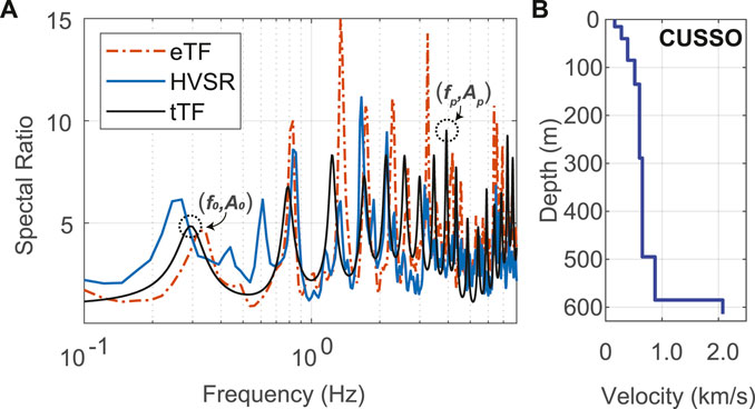
FIGURE 1. (A) S-wave borehole transfer function (eTF), S-wave HVSR, and theoretical (tTF) spectral ratios (1D response) determined at the CUSSO vertical seismic array, whose S-wave velocity profile is shown (B). Multiple peaks and troughs are shown in each spectral ratio demonstrating that site response is frequency dependent. The frequencies and amplifications of the fundamental- (f₀, A₀) and peak- (f_p, A_p) modes on the tTF are indicated.

Site response peaks are extant not only at sites with strong underlying impedance ratios, but also at sites with smoothly varying impedance profiles, or “gradient” sites. Following Boore (2013), Wang and Carpenter (2023) observed such peaks in theoretical and empirical transfer functions, indicating that SH-waves resonate to some degree at sites underlain by impedances that increase with depth yet that lack strong impedance contrasts between layers.

The character of the site response functions for sites that experience resonance varies from simple, with regularly spaced peaks and the largest peak being the first–i.e., the fundamental one—to more complex with irregularly spaced peaks. Carpenter et al. (2020) and Wang and Carpenter (2023) showed that site response functions at sites underlain by a single strong impedance contrast most often demonstrate simple resonance, whereas the site-response functions at those sites underlain by multiple strong impedance contrasts are the more complex ones. These studies also demonstrated that estimating resonance parameters at locations with more than one underlying strong impedance contrast from simplified, one-layer average site profiles, underestimates both the amplifications and the corresponding frequencies.

Although near-surface geologic layers, and thus site response, may vary over relatively small spatial scales, site response is frequently accounted for ergodically using regional or global proxies, particularly so in ground motion models used in seismic hazard assessments. Common amplification proxies are derived from site velocity profiles. The time-averaged S-wave velocity of the upper 30 m (Vs30) remains the most popular (Boore et al., 1997; Stewart et al., 2020), although it has been shown to be inappropriate in certain situations (Castellaro et al., 2008; Hashash et al., 2008; Cadet et al., 2010; Lee and Trifunac, 2010; Régnier et al., 2014; Carpenter et al., 2020). Numerous studies have concluded that including at least one site-specific term greatly reduces ground motion model residuals, particularly at longer periods (e.g., Pitilakis et al., 2013). Popular terms are the depths to a particular S-wave velocity and empirically derived site resonance frequencies. The most common depth-based proxies include Z_1.0 and Z_2.5, i.e., the depths to 1.0 km/s and 2.5 km/s velocity horizons, respectively (e.g., Day et al., 2008). Velocity contrasts (Hou and Zhao, 2022) and impedance ratios (Shingaki et al., 2018) have also been evaluated as site response proxies at seismic stations in Japan and in numerical experiments.

Site response has been extensively studied in well-monitored, seismically active regions such as Japan and California. In the central and eastern United States (CEUS), earthquake rates are much lower and fewer site response investigations have occurred. Thus, more work is needed to characterize CEUS site effects, in large part because many locations in the region sit on unlithified sediments that are underlain by stiff bedrock. At such sites, S-wave resonance is a major concern (Street et al., 1997; Woolery et al., 2008; 2009; Baise et al., 2016; Pratt et al., 2017; Carpenter et al., 2018; 2020; Hassani, and Atkinson, 2018; Sedaghati et al., 2018; Pratt and Schleicher, 2021; Stephenson et al., 2021; Pontrelli et al., 2023), although Vs30 remains a common site attribute to account for site response in the region (Parker et al., 2019; Stewart et al., 2020).

The purpose of this investigation is to characterize linear site response in the CEUS through analyses conducted at seismic stations distributed across the region and to evaluate the skill of various attributes, derived from the site velocity profiles, to predict the primary response characteristics, namely, the frequencies and amplifications of the fundamental modes, f₀ and A₀, and of the peak (i.e., largest) modes, f_p and A_p (Figure 1).

In addition to considering the aforementioned proxies (Vs30, Z_1.0, and Z_2.5), the following equations for the resonance frequencies and amplification at the fundamental mode motivated our evaluation of three additional impedance-based site attributes: the maximum impedance ratio (IR), IRmax, the depth to IRmax, Z_IRmax, and the time-averaged Vs to Z_IRmax, Vs_IRmax.

Equation 1 relates the linear, vertical-incidence SH-wave resonance frequencies with a single-layer Vs profile (Haskell, 1960),

${\stackrel{\sim }{f}}_n=\frac{Vs}{4\bullet Z_b}\ast \left(2\bullet n+1\right),n=0,1,\dots (1)$

where Z_b is depth to the base of the surface layer (or equivalently the thickness of that layer) with velocity Vs, which could correspond to bedrock or another strong impedance contrast. Equation 1 indicates both that depth- or (equivalently) thickness-based and velocity-based parameters control site resonance frequencies and that these frequencies are directly related to Vs and inversely related to depth (or thickness).

Dobry et al. (2000) showed that the following equation well estimates A₀ in the case of linear 1D site response for a single layer over a bedrock half-space:

${\stackrel{\sim }{A}}_0=\frac{1}{\left({\mathrm{I}\mathrm{R}}_{bs}^{-1}\right)+\frac{\mathrm{\pi }\bullet {\mathrm{\gamma }}_{\mathrm{s}}}{2}},(2)$

where IR_bs is the bedrock-sediment impedance ratio (see Equation 3, below) and ${\mathrm{\gamma }}_{\mathrm{s}}$ is the S-wave damping factor. In the absence of S-wave damping, Equation 2 shows that ${\stackrel{\sim }{A}}_0$ = IR_bs, whereas the relationship is nonlinear when damping is included. Although ${\mathrm{\gamma }}_{\mathrm{s}}$ reduces ${\stackrel{\sim }{A}}_0$, Carpenter et al. (2020) showed that the impedance ratio has a much larger influence on ${\stackrel{\sim }{A}}_0$ than the term which includes S-wave damping, i.e., $\mathrm{\pi }\bullet {\mathrm{\gamma }}_{\mathrm{s}}/2$.

We thus evaluated correlations between the primary response parameters and site-specific depth, velocity, and impedance-based attributes. We also characterized the sites based on impedance ratio distributions—single-layer, multilayer, and gradient—and evaluated the strengths of the parameter-proxy correlations for the different site types.

Our correlation analyses were based on theoretical calculations rather than on empirically derived site responses. These calculated site responses thus depend directly on the very Vs profiles from which the proxies were derived and therefore factors related to inaccurate site models and unreliable comparisons with empirical site responses are not concerns.

Finally, we also evaluated the reliability of empirical site response estimations from S-wave HVSR analyses at certain sites. Numerous studies have demonstrated that HVSR of earthquake waves can measure f₀ (e.g., Zhu et al., 2020a; Schleicher and Pratt, 2021). Carpenter et al. (2020) also suggested that A₀ could be approximated by the S-wave HVSR ordinate at f₀ after applying a simple correction. We also evaluated whether S-wave HVSR is useful to characterize underlying impedance-ratio distributions, to assist with applying the most appropriate site-response predictor at a given site.

2 CEUS seismic stations and site attributes

We identified 89 temporary and long-term CEUS seismic stations in the scientific literature that had near-surface S-wave velocity structures into seismological bedrock available (Supplementary Table S1, available in the Electronic Supplement to this article). In this study, we define bedrock as Vs = 760 m/s. All stations operated at least one broadband sensor at the free surface, most of which were seismometers; as needed the recordings from strong-motion accelerometers were analyzed when available. As Figure 2 shows, the stations sit in a variety of geological conditions from outcropping bedrock in the Appalachian Mountains, to shallow and relatively thin unconsolidated sediments overlying deep sedimentary basins (e.g., Anadarko and Illinois Basins), to thick unlithified deposits in the Mississippi Embayment and Atlantic Coastal Plain. For all stations identified, we attempted to calculate earthquake S-wave horizontal-to-vertical spectral ratios, which we could determine for all but 21 of these stations.

FIGURE 2

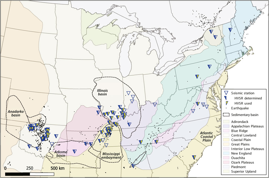
FIGURE 2. Generalized physiographic provinces and seismic stations used in this investigation. Theoretical analyses were conducted for all stations. S-wave HVSR analyses were conducted at stations designated by blue half-triangles; HVSRs from only those stations marked with yellow half-triangles were used in comparisons with the 1D results. Sedimentary basins beneath or near seismic stations are also shown and labeled. Earthquakes used for HVSR analyses are shown as small filled circles.

We collected S-wave velocity (Vs) profiles for each station, which are available in the Supplementary Material and plotted in Supplementary Figure S1. From these profiles, we calculated or extracted the IRmax, Z_IRmax, Z_1.0, Z_2.5, Vs30, and Vs_IRmax attributes. Distributions of these attributes are shown in Figure 3.

FIGURE 3

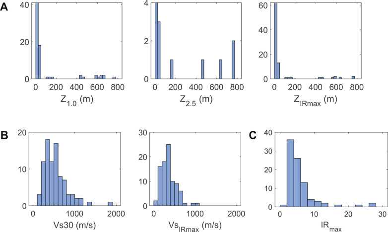
FIGURE 3. Distributions of site attributes extracted or derived from the Vs profiles used in this study: (A) Depth-based attributes; (B) Vs-based attributes; and (C) maximum impedance ratio.

3 Methods

3.1 Average velocities and IRmax-based proxies

All average velocities were calculated as the time-weighted average, i.e., depth to the horizon of interest divided by the total travel time for a vertically ascending S-wave, where the total travel time is the sum of the layer travel times. To calculate layer impedances, we first estimated layer densities (ρ) using the ρ(Vs) relationship in Boore (2016). Then impedance ratios were calculated at each Vs-profile interface as the ratio of the impedance of the underlying layer to average impedance of the overlying layers (Wang and Carpenter, 2023):

${IR}_j=\frac{{Vs}_j^{-}\bullet {\rho }_j^{-}}{\overline{{Vs}_j^{+}}\bullet \overline{{\rho }_j^{+}}}(3)$

where $\overline{{Vs}_j^{+}}$ and $\overline{{\rho }_j^{+}}$ are the time-averaged Vs and thickness-average ρ of the layers above the j^th interface and ${Vs}_j^{-}$ and ${\rho }_j^{-}$ are the Vs and ρ of the layer immediately below the j^th interface. IRmax is defined as the largest impedance ratio at a site, Z_IRmax is the depth to that interface, and Vs_IRmax is time-averaged Vs above that interface.

3.2 1D site response parameters

Using the collected Vs-profiles as input, we calculated 1D site response using the matrix propagation method of Haskell (1953); Haskell, (1960). This methodology has been used widely and in the CEUS (Carpenter et al., 2018; Carpenter et al., 2020) to calculate one-dimensional linear elastic SH-wave amplification functions for input velocity profiles and other dynamic parameters. Thus, we used this method to calculate theoretical site responses at each site in this investigation. We modeled vertically incident SH-waves, incorporating viscoelastic effects through complex shear moduli in each layer, similar to Joyner et al. (1976), and we refer to the resultant theoretical amplification functions as the 1D responses.

The density profiles developed to calculate the impedance ratio profiles were also used in the 1D site response calculations. Viscoelastic effects were accounted for using Q_ef, the effective S-wave quality factor. We follow Campbell (2009), who interpreted Q_ef in eastern North America as frequency-independent and calculated as the inverse of the summed intrinsic and scattering S-wave attenuations in near-surface layers. We used relationships between Q_ef and Vs developed for the central and eastern U.S. by Wang et al. (1994), equations 20 and 21, therein, and Campbell (2009), equations 14 and 15 therein, to estimate Q_ef for each layer in each Vs profile. We then calculated ${\mathrm{\gamma }}_{\mathrm{s}}$, the S-wave damping ratio, for each layer from $Q_{ef}$ using (Campbell, 2009)

${\mathrm{\gamma }}_s=\frac{1}{2Q_{ef}}.(4)$

Carpenter et al. (2020) demonstrated that the range of γ_s estimated from the four Q_ef(Vs) models and Equation 4 is small at the 11 CEUS sites they evaluated, which were on a variety of underlying geologies. Thus, we calculated the final ${\mathrm{\gamma }}_s$ for each layer at each site, except the two deep vertical seismic arrays in the upper Mississippi Embayment, VSAP and CUSSO, by applying Equation 4 on the arithmetic mean of the four Q_ef(Vs) estimates determined for a particular layer. For VSAP and CUSSO (further discussed below), we estimated Q_ef for each layer using equations 20 and 21 in Wang et al. (1994), which respectively were developed for those sites, and then applying Equation 4.

We extracted the first and peak frequencies, f_0,1D and f_p,1D, and corresponding amplifications, A_0,1D and A_p,1D, from the 1D responses, as shown in Figure 1, for evaluation.

3.3 Empirical site response parameters from S-wave HVSR

Earthquake HVSR, which has been shown to approximate site response at some sites (Lermo and Chávez-García, 1993; Sedaghati et al., 2018; Carpenter et al., 2020), is the ratio of the horizontal-component amplitude spectrum divided by the vertical-component’s amplitude spectrum calculated from seismograms of local and regional earthquakes. For each of the stations with identified Vs-profiles except CUSSO and VSAP we acquired and processed available recordings of magnitude 2.5 and greater earthquakes within 3.0 degrees of a given station from EarthScope (www.ds.iris.edu/ds/nodes/dmc/). To avoid any effects of nonlinearity on the empirical spectral ratios, we used only three-component recordings with peak ground accelerations of less than 25 cm/s². For CUSSO and VSAP, we used the same weak-motion dataset that Carpenter et al. (2018) used, consisting of triggered earthquake recordings. Our S-wave HVSR processing involved estimating site fundamental frequencies from preliminary HVSR curves, which we used to establish site-specific processing parameters for the final S-wave HVSRs. We evaluated resonance frequencies and spectral ratio values measured on the final curves.

Preliminary and final S-wave HVSRs were processed following nearly the same steps and as follows: 1. Calculate S-wave and noise window lengths, which, as discussed below, differed between the preliminary and the final processing. 2. Calculate the individual-earthquake amplitude spectra from the windowed, de-trended (i.e., linear trends removed), and tapered three-component S-wave time series after removal of the instrument responses. 3. Calculate pre-P-wave noise amplitude spectra using identical processing parameters and procedure. 4. Smooth the S-wave and noise amplitude spectra; the smoothing approaches differed between the preliminary and final processing as expounded below. 5. Determine reliable S-wave spectral amplitudes at each frequency via signal-to-noise ratios (SNR), where SNR is a function of frequency and is calculated by division of the signal spectrum by the noise spectrum; spectral components with SNR < 2.0 were rejected (following Carpenter et al., 2020). 6. Calculate individual-event HVSRs as the ratios of the horizontal-to-vertical S-wave amplitude spectra but only at frequencies where each component’s SNR is ≥ 2.0. 7. Form the site’s S-wave HVSR as the arithmetic mean from a minimum of three but up to 50 individual-event spectral ratios at each frequency, following the procedure described in Carpenter et al. (2020). 8. Measure resonance frequencies and spectral ratios from the mean HVSR peaks that have prominences of at least 1.0. In other words, HVSR peaks were ignored if their heights above either of their bounding troughs were less than 1.0.

To estimate sites’ fundamental resonance frequencies for final HVSR processing, we attempted to determine preliminary S-wave HVSRs at each site. As expounded in the Supplementary Material to this article, we used fixed-length 60 s S-wave windows to process the preliminary HVSRs, where individual-component S-wave amplitude spectra were smoothed using a Konno-Ohmachi smoother (Konno and Ohmachi, 1998). At some sites, no clear peaks were observed in the preliminary HVSRs. At some other sites in or near sedimentary basins, peaks were observed at unreasonably low frequencies when compared with the predicted 1D responses. Such low-frequency peaks have been attributed to S-wave resonances between the surface and rock layers well below the bases of the Vs profiles determined at these or nearby stations (Mendoza and Hartzell, 2019; Carpenter et al., 2020). The presence of such peaks rendered identifying the first peaks due to the characterized near-surface layers as ambiguous. Figure 4 shows examples of these types of preliminary HVSR curves from seismic stations in Oklahoma, United States. The HVSR curve at OK009 has an unambiguous peak that can be associated with the characterized near-surface Vs structure whereas the spectral ratio at OK032 has two clear peaks. The first peak occurs at a frequency (∼1 Hz) and is much lower than the f_0,1D predicted by 1D modeling (∼5.6 Hz), suggesting site response is affected by deeper geological layers at this site. The HVSR curve for OK001 has no peaks with significant prominence.

FIGURE 4

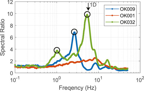
FIGURE 4. HVSR curves developed for three sites. Circles indicate strong peaks in the HVSRs. The inverted arrow indicates the frequency of the first peak at OK032 determined from 1D modeling.

To process the final HVSRs, we used site-specific window lengths of at least 10/f_0,HV seconds (similar to the SESAME standards (SESAME project, 2004)), where f_0,HV is the frequency of the first peak on the preliminary site HVSRs, to capture any S-wave reverberations in the near-surface layers. For sites with no clear peaks or with ambiguous first peaks, we assigned a default S-wave window of 10.0 s under the assumption that near-surface, characterized layers would not significantly amplify SH-waves at frequencies lower than 1.0 Hz. The selection of 1.0 Hz is consistent with the peaks seen in HVSRs determined for stations in the same region whose HVSRs appear to be unaffected by deeper structure. S-wave spectra for the final HVSRs were smoothed with running Hanning windows of site-specific lengths f_0,HV/2 Hz. For sites processed with the default window length of 10.0 s, we used Hanning windows of length 0.5 Hz.

The fundamental-mode and peak frequencies, f_p,HV, and corresponding spectral ratios, A_0,HV and A_p,HV, respectively, were measured from the site S-wave HVSR curves by selecting the first and highest peaks with prominences of at least 1.0. As discussed below, although we conducted HVSR analyses at all stations possible, including those whose preliminary HVSR curves lacked clear peaks, we decided ultimately to exclude the HVSR curves with ambiguous first peaks from the final analyses.

4 Results

Theoretical 1D site response functions and empirical S-wave HVSR curves are shown in Supplementary Figure S2 and the extracted primary site-response parameters are listed in Supplementary Table S2. There is a broad range of resonance frequencies predicted for the CEUS, consistent with the empirical observations in Yassminh et al. (2019). Figure 5 shows that both f_0,1D and f_{p, 1D} span more than two orders of magnitude, with the lowest resonance frequencies of 0.2 and 0.3 Hz for f_0,1D, f_p,1D, respectively. These low resonance frequencies occur at sites in the upper Mississippi Embayment and the Atlantic Coastal Plain with underlying thick (100 m to 845 m) sediment deposits. At 10 sites, fundamental-mode resonances occur at frequencies greater than 20 Hz, i.e., higher than the frequencies typically of concern for engineering purposes, and the peak-modes at 26 sites occur at frequencies greater than 20 Hz. Amplifications of up to 13.2 are predicted for one site, although amplifications at f_0,1D at most sites are around 5 (mean A_0,1D = 5.1; median A_0,1D = 4.5); peak amplifications at most sites are around 6 (mean A_p,1D = 5.8; median A_p,1D = 5.6).

FIGURE 5

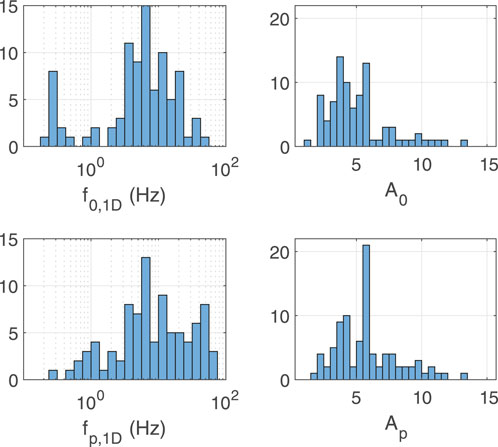
FIGURE 5. Distributions of theoretical site resonance parameters determined at the 89 CEUS seismic stations.

4.1 Parameter-proxy relationships

The theoretical primary site response parameters, f_0,1D, f_p,1D, A_0,1D, and A_p,1D, were gathered from the 1D responses (Supplementary Table S2), and the proxies were derived from the site Vs profiles (Supplementary Table S2; Figure 3). To explore the parameter space, we first generated scatter plots of each proxy-parameter pair, shown in Figures 6, 7. We evaluated fits to the parameter-proxy pairs, also shown in Figures 6, 7, using linear and two- and three-parameter power laws of the form $y=c\bullet x^d$ and $y=c\bullet x^d+e$, respectively, where c, d, and e are free model parameters. The frequency-based parameters and depth-based proxies are in logarithmic (base-10) units for the linear fits.

FIGURE 6

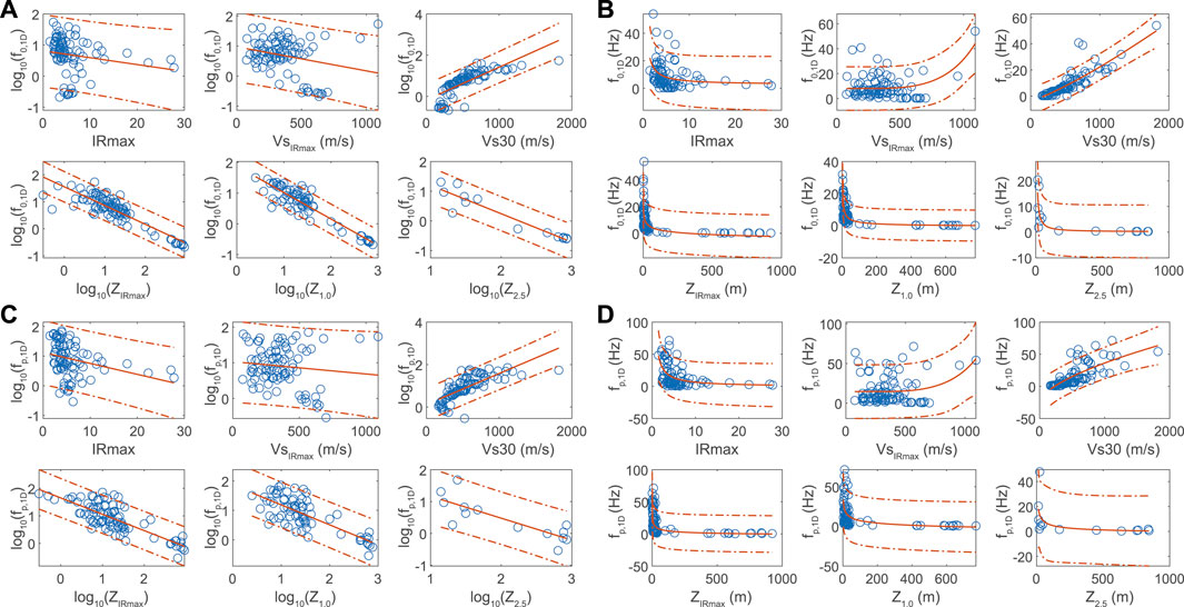
FIGURE 6. Scatter plots of all proxies and frequency-based parameters, best-fit lines and power-law functions, and the 95 percent prediction intervals. Linear models involving f₀ (A) and f_p (C) and power-law models f₀ (B) and f_p (D) are shown.

FIGURE 7

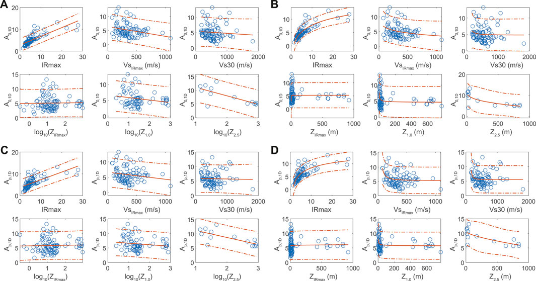
FIGURE 7. Scatter plots of all proxies and amplification-based parameters, best-fit lines and power-law functions, and the 95 percent prediction intervals. Linear models involving A₀ (A) and A_p (C) and power-law models A₀ (B) and A_p (D) are shown.

Site resonances can occur at lower (<1 Hz) and at higher frequencies (≥1 Hz) at deep- and at shallow-soil sites. For example, as listed in Supplementary Table S2, EVIN and VSAP have equal f_0,1D (1.2 Hz) and similar Vs30 of 332 m/s and 289 m/s, respectively, yet these sites have very different Z_1.0 of 36 m and 100 m, respectively and different f_p,1D of 1.2 Hz and 5.1 Hz, respectively. As another example, Z_1.0 at LPAR and MCIL differ by approximately an order of magnitude (657 m versus 20.5 m, respectively) as do their f_0,1D (0.3 Hz and 1.9 Hz, respectively), yet these sites also have nearly equal Vs30 (205 m/s and 218 m/s, respectively) and f_p,1D (1.8 Hz and 1.9 Hz, respectively). Additionally, A_0,1D and A_p,1D, respectively are factors of approximately 2 and 2.5 greater at MCIL than at LPAR. Thus, sites with similar near-surface characterizations may have very different deeper subsurface characteristics that affect site resonance. Therefore, separately regressing subsets of proxy-parameter pairs based on, e.g., depth, frequency, or other, may inadequately characterize the relationships and associated uncertainties. In addition, some recent studies have argued that the near-surface attribute Vs30 is suitable as a site proxy even in settings such as the CEUS where deep geologic layers contribute to site response (e.g., McNamara et al., 2015). To provide a more reliable characterization of the site-response parameter uncertainties that could be encountered across the CEUS, we felt it important to evaluate all proxies using the full range of site-response parameters.

As with the linear scatter plots, we took the base-10 logarithm of the frequency- and depth-based variables prior to fitting the linear models. Table 1 lists goodness-of-fit metrics for the linear and power-law models. The best-fitting linear and power-law models’ parameters are listed in Supplementary Tables S3, S4, respectively. Compared to the three-parameter power-law model, the two-parameter power-law model generally yielded a similar or poorer fit to the parameter-proxy pairs and was not considered for subsequent comparisons and discussion.

TABLE 1

TABLE 1. Number of points and goodness-of-fit metrics for linear and power-law models for all proxy-parameter pairs.

Based on the greatest R² values (we used adjusted R², as opposed to non-adjusted R², which accounts for the number of degrees of freedom and allows more meaningful comparisons of the goodness-of-fit between models with differing numbers of free parameters (James et al., 2013)), the linear model is preferred to the power-law models for frequency-depth parameter-proxy pairs, whereas the power-law model is preferred for almost all other pairs. The strongest correlations (i.e., the Pearson’s correlation coefficient) are between depth-based proxies and f_0,1D, with Z_2.5 being the strongest. The same is true for peak frequency, although the correlations are slightly weaker than for fundamental frequency. Apparently, Vs30 also relates to f_0,1D and f_p,1D, with the strength of the former power-law relationship being much stronger than that of the latter.

Amplifications generally have weaker relationships with the various proxies than frequencies, and only IRmax can be considered to have robust and strong relationships (R² ≥ 0.5) with amplification. Although Z_2.5 appears to linearly correlate with A_0,1D, the 95% prediction bounds are quite large (∼±5) at all depths (in this study, the prediction intervals quantify the confidence associated with the fitted curve and depend on the inverse of the Student’s t cumulative distribution function and the variability of a new observation as quantified by the mean squared error). More data may assist with improving the robustness of the Z_2.5 versus amplification relationships. Our analyses indicate that Vs30 does not correlate with amplification in our study area.

4.2 S-wave HVSR

We refer to the first and largest peaks in the S-wave HVSR curves as A_0,HV and A_p,HV, respectively, which occur at frequencies of f_0,HV, and f_p,HV, respectively. To avoid the possible influence of deeper structure, such as in or near basins, on the empirical spectral ratios we opted not to include the peaks selected at sites where the first peak was ambiguous. In addition to the examples given in Figure 4, Supplementary Figure S4 presents additional HVSR curves with significant peaks that occur at frequencies well below those predicted by the 1D responses. Although such peaks may represent a lack of Vs-profile resolution in the near surface, they have been observed in Oklahoma by Mendoza and Hartzell (2019), and elsewhere in the CEUS (Yassminh et al., 2019; Carpenter et al., 2020) where they were attributed to deeper sedimentary strata. Additionally, no peaks were observed on some S-wave HVSRs most likely because no significant impedance contrasts underlie the corresponding sites (e.g., OK001 in Figure 4). In total, we measured clear peaks in the S-wave HVSR curves developed at 36 of the 72 stations with sufficient earthquake recordings, which are listed in Supplementary Table S5.

Figure 8 compares the first- and peak-frequencies measured from the S-wave HVSR curves with those determined through the 1D analyses at the 36 seismic stations. In general, the empirical measurements agree well with the first- and peak-frequencies calculated through the 1D analyses, particularly after excluding the frequencies of the first peaks measured at sites suspected to be influenced by deeper structure (Figure 8A). The comparison between f_0,1D and f_0,HV is particularly strong (r=0.90; p=0.00), showing that S-wave HVSR has skill to estimate the fundamental resonance frequencies at these sites, assuming the Vs profiles are reasonably accurate. The comparison of the frequencies of maximum amplifications, f_p, is more scattered (r=0.47; p=0.00) and shows that the calculated peak frequencies tend to be greater than those measured with HVSR. A likely explanation of this is that at frequencies greater than f₀, HVSR tends to decrease relative to the site transfer function (Rong et al., 2017; Carpenter et al., 2018; Zhu et al., 2020b). Thus, at sites where f_p,1D > f_0,1D, the first HVSR peaks are more likely to be the largest peaks. In fact, at all except for seven sites, f_p,HV = f_0,HV (Figure 8B), whereas f_p,1D = f_0,1D at only 18 of the same 36 sites. Therefore, the utility of HVSR to estimate the site-response parameters may be limited to the fundamental modes.

FIGURE 8

FIGURE 8. Comparisons of the first- (A) and peak-frequencies (B) measured from S-wave HVSR and calculated from 1D analyses at the 36 sites with unambiguous first HVSR peaks. Peaks picked on the sites with ambiguous first peaks, possibly influenced by deeper structure (cf. Supplementary Figure S4) and excluded from analysis, are also shown in (A) as open circles. (C) Comparison of the spectral ratios at f_0,HV. The 1:1 lines are shown for comparison and Pearson correlation coefficients are also included.

Figure 8 also compares the spectral ratios at f₀. There is much more scatter in the A₀ comparison than in the frequency comparisons, much of which could arise from large variabilities observed in HVSR at site resonance frequencies (e.g., Carpenter et al., 2018). Nevertheless, there is a positive, albeit weak correlation (r=0.35; p=0.04) between the empirical and theoretical spectral ratios at f_o. We do not compare A_p,HV and A_p,1D since we observed that f_p,HV and f_p,1D do not correspond at numerous sites (Figure 8B, Supplementary Figure S2).

5 Discussion

The correlation results using parameters derived from the 1D analyses indicate that at these CEUS sites, not all proxies are related to the site response parameters. It is also apparent that no single proxy is related to both frequency- and amplification-based response parameters. Thus, predicting both the resonance frequencies and corresponding amplifications at a site requires two predictors.

5.1 Predicting f₀ and f_p

The results reveal site fundamental- and peak-resonance frequencies can be well predicted from the depths to the 1.0 km/s velocity horizon and from the depth to the maximum impedance ratios in the Vs profiles. The depth of the 2.5 km/s horizon has the strongest relationship with these frequency parameters. These favorable frequency-depth results are consistent with findings in other studies that demonstrated strong correlations between depth-f pairs of variables globally (e.g., Yamanaka et al., 1994) and in the CEUS (e.g., Schleicher and Pratt, 2021; Zhu et al., 2021) and are expected based on Equation 1. Although, in reference to Equation 1, it was also expected that Vs_IRmax would be related to frequency, the regression results indicate that there is no relationship between fundamental or peak frequency and Vs_IRmax. We considered the possibility that the average Vs to other horizons might result in stronger correlations, and thus also evaluated the average Vs to depths of Z_1.0 and to Z_2.5 against f_0,1D and f_p,1D. However, the coefficients of determination were lower than those from the Vs_IRmax regressions indicating that these average-Vs attributes are unreliable as resonance proxies.

Interestingly, although each depth-based proxy has a large value range of more than two orders of magnitude (Figure 3), Vs30 — which characterizes just the upper 30 m—correlates with f_0,1D. The strength of the relationship, which has been observed in other studies in the region (McNamara et al., 2015; Hassani and Atkinson, 2016) and has a relatively large R² of 0.73 in our dataset, which may be due at least in part to most sites having Vs characterized to 30 m depth or less (n = 55). However, the strength of the relationship belies potential problems with reliably predicting f₀ at low Vs30 (166 m/s to ∼400 m/s) values, where amplification effects may be of greatest concern.

As Figure 9 shows, the f_0,1D-Vs30 residuals are relatively small at low-Vs30 (Figure 9B), but as shown in Figure 9C, the percentage of f_0,1D that the residuals constitute is the very large at Vs30 less than ∼400 m/s. Thus, predicting resonance frequencies using Vs30 at low-Vs30 sites is highly uncertain. Also, as Figure 9 shows Vs30 alone does not distinguish shallow soil from deep soil sites, where Vs30 is most often low and wave propagation effects, particularly at f₀, differ greatly from shallow sites (e.g., Hashash et al., 2008). As Figure 9 shows, all but one of the 15 sites with thicker-sediments (depth to the base of the Vs-profile layers ≥ 50 m) have low Vs30 and these same sites have the largest percent residuals (up to 1,100% of f_0,1D).

FIGURE 9

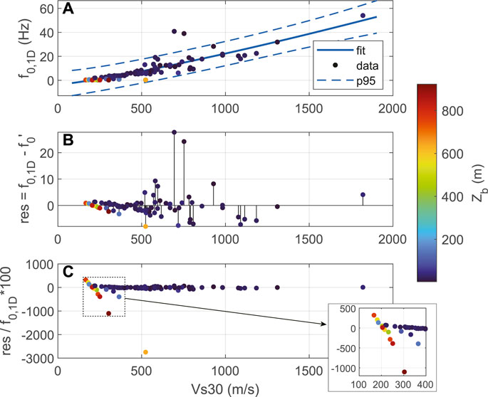
FIGURE 9. Performance of the f_0,1D–Vs30 regression, with a focus on residuals at lower-Vs30. Points are colored by the depth of the Vs profiles, Z_b. (A) Best fitting power-law function to the Vs30-f_0,1D data and the ±95% prediction intervals (p95). (B) f_0,1D residuals (1D-calculated minus predicted) relative to the fit in (A). (C) Percentage residual-to-f_0,1D. The inset box is the lower-Vs30 subset (from 100 to 400 m/s).

Plots analogous to those in Figure 9 for linear f_0,1D–Z_1.0 and f_0,1D–Z_IRmax regressions are given in Supplementary Figure S5. Notably, not only are the residuals for these regressions lower overall than those derived from Vs30, but the residuals are much smaller in terms of percent f_0,1D, indicating that both Z_1.0 and Z_IRmax are much more appropriate for predicting fundamental resonance frequencies than Vs30.

As listed in Table 1, strong (R² ≥ 0.5) relationships between the same proxies—Vs30, Z_1.0, and Z_IRmax—were found for f_p, also with power (Vs30 only) and linear relationships. Also, we observed the same residual trends for f_p versus Vs30 compared with f_p versus the depth-based proxies: chiefly that peak-frequencies at deep-soil sites are uncertain for the Vs30 relationship and the depth-proxies yield improved residuals overall relative to Vs30. However, the goodness-of-fit metrics for all relationships with f_p were less than those for f₀ (Table 1).

Although the relationships between the frequency parameters and Z_1.0 (f₀ and f_p) and Z_2.5 (f₀ only) are strong, the depth to the maximum impedance ratio is as well strong but also has an important advantage over the other two: Z_IRmax can be determined at any site with a measured Vs-profile, whereas, Z_1.0 and Z_2.5 require estimations of the depths to those Vs horizons that may be unknown or can be estimated only with large uncertainties.

5.2 Predicting A₀ and A_p

We found that only one parameter, the maximum impedance ratio, has a strong relationship (R² ≥ 0.5) with fundamental and peak amplifications. This is expected when considering the expression for the 1D amplification at f₀ for a single layer over a half-space given in Eq. 2: Equation 2 predicts that A_0,1D would likely relate strongly to IRmax, particularly for sites underlain by a single strong impedance ratio. Our 1D calculations include viscoelastic effects and thus, as expected (because most sites are underlain by a single strong impedance contrast), the power-law relationship fits the A_0,1D—IRmax ordered pairs better than the linear model (Table 1). The same is true for the A_p,1D—IRmax ordered pairs, however the power-law fit for this pair is of slightly lower quality.

5.3 Reanalysis considering impedance-profile characteristics

Carpenter et al. (2020) identified situations where Eqs. 1, 2 provide poorer approximations of fundamental-mode resonance frequencies and amplifications calculated by 1D analyses. They found that ${\stackrel{\sim }{f}}_0$ and ${\stackrel{\sim }{A}}_0$ are respectively less consistent with f_0,1D and A_0,1D at sites underlain by more than one strong impedance contrast. Wang and Carpenter (2023) showed that the consistency further decreases for sites whose Vs-profiles are best characterized as gradient-like, i.e., lacking strong impedance ratios. To expand the findings in those studies and to explore further the effects that the number and magnitudes of underlying impedance ratios have on the calculated primary site response parameters, we categorized each Vs profile based on the number of strong impedance ratios, i.e., 3.0 or greater, although other ratios could be evaluated. We assigned a Vs-type of 1L, ML, UL, G, or B to each profile: 1L–single layer, a single strong impedance ratio; ML–multilayer, two or more strong ratios; UL–upper layer, a single strong ratio, but which occurs at significantly shallower depth than the base of the Vs-profile, namely, less than half the depth; G–gradient, multiple layers in the Vs profile but no strong impedance ratios; and B–bedrock, no strong ratios and all layers’ Vs of at least 760 m/s. Figure 10 shows examples of each Vs-type and gives the distribution of assigned Vs-types. Because there are so few UL (2) and B (1) sites, we only investigated regressions using site response parameters and proxies at 1L, ML, and G sites.

FIGURE 10

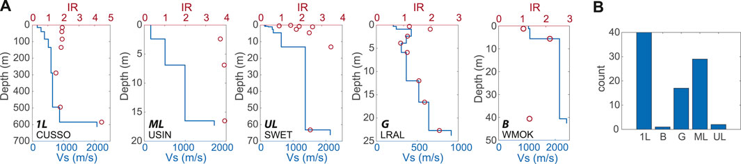
FIGURE 10. (A) Examples of Vs- and impedance-ratio- (IR) profiles for the five categories used to classify Vs-types. Plots are labeled with categories 1L, ML, UL, G, and B, and with the station names. (B) Distribution of Vs-types at the sites used in this investigation.

We repeated the linear and power-law model regressions for the 1L, ML, and G Vs-types and present the models’ parameters in Supplementary Tables S6—S11. Comparisons of the linear versus power-law fits for the Vs-type subsets are given in Supplementary Table S12 and a summary of the best-fitting models’ parameters is given in Table 2. The results reveal that analyzing subsets of the dataset based on Vs-type may improve the regressions as quantified by both increasing R² values and decreasing the standard errors. Notably, all regressions are strengthened for single-layer Vs-types. About half of the regressions are strengthened for multilayer sites. For gradient sites, only the single A_p,1D - IRmax pair has a strong relationship.

TABLE 2

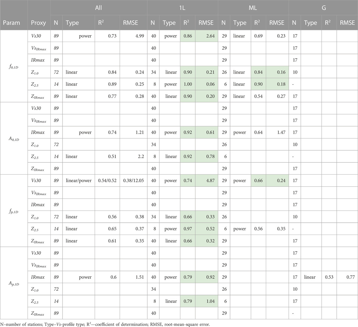
TABLE 2. Comparisons of goodness-of-fit parameters among the best-fitting models for each Vs-profile type. Models for which both the coefficients of determination and the standard errors are improved compared to the base-case of all Vs-profile-types are highlighted.

In Figure 11, we show ordered pair subsets by Vs-type and corresponding best fit relationships for the IRmax-based proxies and each site response parameter. The trends of the fits are consistent regardless of Vs-type, but the ordered pairs are more scattered for multilayer and gradient sites than for single-layer sites. This figure also illustrates that the largest amplifications predicted for this dataset are produced at sites underlain by multiple strong impedance contrasts and that the longest-period resonances occur at single-layer sites.

FIGURE 11

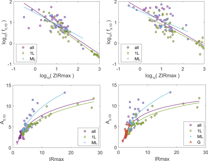
FIGURE 11. Relationships between site-response parameters and IRmax-based proxies for all ordered pairs and for subsets based on Vs-types 1L, ML, and G. Only those relationships with R² ≥ 0.5 are shown. The colors of the best-fitting models match the colors of the corresponding ordered pairs.

5.4 Utility of S-wave HVSR

Because many of the regressions improved when calculated on data subsets based on Vs-type, we reevaluated the parameters picked on the S-wave HVSR curves for the various types. Because some site characterization surveys were conducted at large distances from the seismic stations, and because Vs-structure can vary rapidly over short distances (e.g., Thompson et al., 2009; Hallal and Cox, 2021), we first attempted to identify sites with accurate average Vs profiles. We applied a strategy similar to that used by Pilz and Cotton (2019), who identified KiK-Net sites with reasonable Vs profiles as those with correlation coefficients between empirical and theoretical borehole transfer functions at the fundamental mode of 0.5 and greater. Carpenter et al. (2018) observed in our study area that S-wave HVSR curves are similar to empirical and theoretical site response functions at the fundamental frequencies at sites with accurate Vs profiles. Under the assumption that this observation from Carpenter et al. (2018) is applicable to each of the 36 sites for which we developed S-wave HVSR curves, we calculated Pearson (r) and Spearman (ρ) correlation coefficients for the HVSR curves against the corresponding 1D responses in site-specific frequency bands from 0.5*f_0,HV to 3*f_0,HV. By rejecting sites where either r < 0.5 or ρ < 0.5, we gained confidence that the sites we analyzed have reasonable Vs profiles on average and thus the extracted frequencies and spectral ratios are suitable for comparison against the proxies at these sites. We found only 19 sites that were suitable for such analyses: 15 single-layer, 2 multilayer, 1 upper-layer, and 1 gradient.

Figure 12 compares the fundamental-mode site-response parameters from HVSR and 1D. It is no surprise that the f₀ parameters are consistent since we required that the theoretical and empirical spectral ratios correlate well around f_0,HV. Therefore, drawing frequency-based conclusions requires additional, independent analyses to confirm the reliability of the site Vs profiles. For this reason, and because f_0,HV has been shown to reliably estimate f_0,1D in numerous studies, as discussed in the Introduction, our HVSR discussion focuses on A₀. The scatter in the A₀ ordered pairs is reduced compared to all the pairs (Figure 8) and there is an improvement in the correlation (r=0.52; p=0.02). These results suggest that S-wave HVSR curves can provide a first-order estimation of A_0,1D and the best-fitting linear relationship is

$A_{\mathrm{0,1}D}=0.4\bullet A_{0,HV}+3.1.(5)$

FIGURE 12

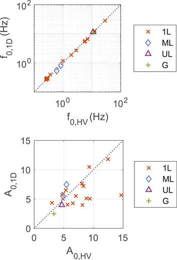
FIGURE 12. Comparisons of f₀ and A₀ from 1D calculations and measurements from S-wave HVSR for the sites with HVSR curves that correlate well (r≥0.5 and ρ≥0.5) with the 1D responses.

Figure 13 presents example S-wave HVSR curves for each Vs type at sites where Vs is well characterized. The close match between the empirical and theoretical curves suggests that S-wave HVSR reflects characteristics of the 1D site response functions. The only example of a bedrock site (station WMOK) was included even though it was not compared in Figure 13 (since f_0,HV could not be determined for this station).

FIGURE 13

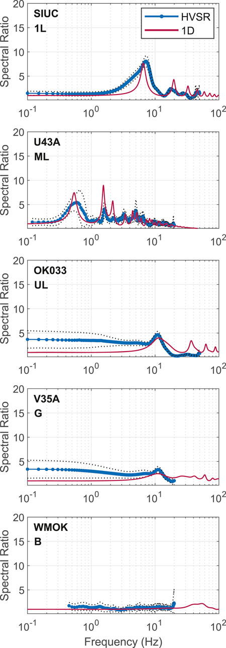
FIGURE 13. Example S-wave HVSR curves (blue) and 1D site-responses for each of the Vs-types characterized in this study.

The examples shown in Figure 13 also suggest that S-wave HVSR curves differ by site type. The HVSR curve at SIUC (1L site) has regularly spaced peaks—i.e., the peaks occur at approximately odd multiples of the fundamental frequency, as predicted by Equation 1—that diminish with increasing frequency, as predicted for a single layer over a half-space. The HVSR curve at U43A (ML site) is more complex, with irregularly spaced peaks—i.e., the HVSR peaks are not separated by an approximately constant frequency interval—and with a relatively high peak (≥5) indicating the presence of at least one larger impedance ratio beneath the station. For OK033, the UL example, only a single clear HVSR peak of value 4.0 is apparent, which occurs at a relatively high frequency of 11 Hz. Peaks at higher frequencies are expected at OK033 but may not have been observed due to data sampling limitations. The HVSR curves, as well as the site transfer functions, at UL sites may resemble those at 1L or ML sites. The largest peak at the G site V35A is much less than the peaks observed at the sites underlain by at least one strong impedance ratio, corroborating that the site lacks a strong underlying impedance contrast. Unfortunately, the Nyquist frequency limits evaluation of the HVSR at frequencies greater than 20 Hz at V35A, but comparing curves at another G site at f >> f_0,HV and with a higher Nyquist frequency, OK009 (Supplementary Figure S4; OK009 was categorized as a basin site and the f_0,HV had to be excluded from the discussed analyses), indicates that the empirical-theoretical spectral-ratio curves are indeed comparable for this site type. For the B site, WMOK, the HVSR curve is flat, as expected for a site at which little-to-no site response is predicted.

5.5 Study limitations and recommendations

Hashash et al. (2014) recommend a relatively fast velocity as reference site conditions for ground motion models and for predicting site amplifications for the CEUS, in the range 2,700 to 3,300 m/s. However, only nine of the Vs profiles we collected include velocities in this range or faster (the median of the sites’ maximum Vs is 1,524 m/s and 1,134 m/s and 2,129 m/s bound the second and third quartiles of the maximum Vs). Supplementary Figure S3 demonstrates that the amplifications at these nine sites lie in the upper ranges of those determined for all sites. Thus, the distribution of amplifications we determined may not be representative of CEUS amplifications that are referenced to the 2,700 to 3,300 m/s range. Nevertheless, we emphasize that site resonances do not depend on absolute Vs maxima, but rather on impedance ratios as indicated by Eq. 2 and suggested by the amplification versus IRmax relationships, and thus note that even the recommendations from Hashash et al. (2014) may be insufficient to account for site resonance in the CEUS.

Another potential limitation of our study results is related to the IRmax-based relationships we developed. The related concern is that the Vs profiles used in this study may not have reached the depths to all impedance contrasts that contribute to site resonance in the frequency range of engineering interest. Thus, it is possible that either or both IRmax and Z_IRmax are too small at some sites, in which case Vs_IRmax may need to be recalculated. As observed in this study, S-wave HVSR can assist with identifying sites that have deeper unmodeled impedance contrasts of relevance (Figure 13, Supplementary Figure S4). And based on the consistencies between the empirical and theoretical spectral ratios in Supplementary Figure S2, it appears that the Vs profiles at sites with underlying thick sediment deposits in the upper Mississippi Embayment and Atlantic Coastal Plain extend to adequate depths to account for all relevant impedance contrasts. Outside of these domains and as discussed in Sections 4.2 and 5.4, the spectral ratio comparisons (Supplementary Figures S2, S4) suggest that some sites lack the detailed structural models needed to assess important resonances from deeper layers.

Because some sites appear to be subject to lower-frequency, unmodeled resonances, our results will be corroborated or strengthened once additional Vs profiles that account for all relevant impedance ratios become available. Nevertheless, we anticipate that the relationships developed using IRmax-based proxies in our dataset will be useful in the CEUS and perhaps elsewhere, as discussed in what follows.

Relevant to the A_0,1D and A_p,1D versus IRmax relationships, Z_IRmax and IRmax are uncorrelated. Also, the distribution of IRmax used in the regressions is similar to the distribution for high-Vs-max subsets of the dataset (Supplementary Figure S6). Thus, we do not expect that very different relationships for A_0,1D and A_p,1D versus IRmax would be developed if deeper depths and higher Vs (e.g., in the range of the Hashash et al. (2014) recommendation) were reported for all sites.

Related to f_0,1D and f_p,1D versus Z_IRmax, at the 73 sites where Z_1.0 was determined, the maximum impedance contrast occurred at that depth at most sites (53 sites; Supplementary Figure S7) or at shallower depths (14 sites). At just six sites, Z_IRmax was found to be deeper than Z_1.0. Also, at the 14 sites where Z_2.5 was measured, Z_IRmax corresponds with Z_2.5 at all but three sites. Therefore, it is possible that stronger impedance contrasts exist at depths corresponding to Z_1.0, Z_2.5, or deeper, at sites where these depths were not determined.

To assess the extent to which our results involving IRmax and Z_IRmax may differ from those developed at adequately characterized sites, we recomputed the regressions using the best-fitting model types listed in Table 2 for “All” Vs profiles (linear versus power-law) on a subset of 39 sites where S-wave HVSRs were determined at frequencies down to 0.1 Hz (Supplementary Figure S2) and which lacked ambiguous low-frequency peaks. The resultant regressions for this subset (Supplementary Figure S8)—all of which have R² ≥ 0.5—nearly coincide with the relationships derived from the entire dataset. The consistencies of these relationships suggest that the results involving the IRmax and Z_IRmax proxies at all sites are reliable. Nevertheless, it would be beneficial to reassess the strengths of these IRmax-based relationships as additional Vs profiles that account for all relevant impedance ratios become available.

Another potential limitation of our study is that we only considered single proxies to predict single site-resonance parameters. It is possible that multiple regression analyses involving two or more of the proxies we evaluated, and perhaps others we did not consider, would yield improved relationships with the primary site response parameters.

5.6 Summary

The strong correlations revealed in this study support the findings of previous studies that the Z-based proxies can predict resonance frequencies and thus also support the use of Z_1.0 and Z_2.5 as site terms (e.g., Day et al., 2008) in CEUS ground-motion models. The results also demonstrate that ZIRmax may serve the same purpose for locations where Z_1.0 and Z_2.5 are unavailable, although S-wave HVSR observations should be used to identify unknown impedance contrasts that produce unmodeled low-frequency resonances of engineering concern. IRmax correlates strongly with fundamental-mode and peak amplifications, and thus serves as another site term for CEUS ground-motion models. As with Z_IRmax, S-wave HVSRs can be used to ensure that additional large impedance ratios are not present beneath the base of site Vs profiles. The Z-based proxies may be useful in developing design spectra for linear ground motions across appropriate site-specific periods (i.e., the inverse of frequency) since fundamental frequencies determined from weak-motion response spectral ratios and those determined from 1D linear response analyses have been shown to be consistent (Wang and Carpenter, 2023). Also, because the Z-based proxies correlate strongly with resonance frequencies and IRmax correlates strongly with amplification, pairs of Z-based proxies and IRmax can be used to modify predicted bedrock spectral amplitudes at a given site, using the relationships we developed, to include linear site effects. Table 2 indicates that, when possible, relationships developed for “1L” sites should be used for these purposes at sites with simple Vs structures and “ML” should be used at sites with multiple underlying strong impedance ratios to predict f_0,1D using Z_1.0 or Z_2.5, and for f_p,1D using Vs30, but only at higher Vs sites.

6 Conclusion

In this study, we determined theoretical 1D linear site-responses at 89 seismic stations in the central and eastern U.S., where determining the most appropriate methodology to characterize site response is an ongoing work. The stations selected had near-surface S-wave velocity structures into seismological bedrock available, where we define bedrock as Vs = 760 m/s. We found that CEUS S-wave resonances at the fundamental (first)- and peak-modes occur across large ranges of frequencies, each spanning more than two orders of magnitude — 0.21–54.0 Hz and 0.29–71.5 Hz, respectively. Amplifications of ∼5 and ∼6 (median values across the 89 sites) are common at the fundamental frequency and peak modes, respectively; the largest amplification calculated was 13.2.

Using simple regression analyses, we investigated six attributes to predict primary site-response characteristics consisting of the fundamental- and peak-resonance-mode frequencies and the corresponding amplifications. The site-specific attributes were derived from the Vs profiles developed at each station and the primary site response parameters were calculated from 1D linear site-responses analyses using the same Vs profiles and the matrix propagation method. All the depth-based attributes we evaluated, Z_1.0, Z_2.5, and Z_IRmax—respectively the depths to the 1.0 km/s and 2.5 km/s Vs horizons and to the maximum impedance ratios—have strong (R² ≥ 0.5) relationships with fundamental and peak resonance frequencies. We note, however, that Z_IRmax has an important advantage over the other two in that it can be determined at any site with a measured Vs-profile. In contrast, Z_1.0 and Z_2.5 require site characterizations that attained those respective velocities, which are not always feasible with standard characterization techniques, particularly for deep-soil sites. Although the average Vs to the Z_IRmax depth does not correlate with the frequency and amplification parameters, the average Vs in the top 30 m, Vs30, does. However, we determined that the Vs30 parameter may not be appropriate at sites with slow near-surface velocities (Vs30 < 400 m/s), where fundamental-mode resonance frequencies are low (<1 Hz) because the predicted-observed frequency residuals can be very large relative to the magnitude of the frequencies (up to 1,100%). We also found that the largest impedance ratios in the Vs profiles have the strongest correlation with the fundamental and peak amplifications.

The characteristics of the calculated site-response functions vary from simple to complex depending on the distribution of strong impedance contrasts (impedance ratios of 3.0 or greater) beneath a site. Site responses at sites with only one strong impedance contrast are relatively simple functions with regularly spaced peaks compared to the functions calculated for sites with multiple strong contrasts and those that lack any such contrasts. We found that the proxy-parameter regressions can be improved when calculated on subsets of the sites based on simple categories of impedance ratio distributions: single-layer, multilayer, and gradient. Our dataset was especially rich with single-layer sites, i.e., those underlain by a single strong impedance ratio, and the regressions are especially strong for these sites; the regression results for other site types will be strengthened by incorporating additional Vs profiles as they become available.

To estimate the site response parameters at these seismic stations empirically, we measured the frequencies and spectral ratios of the first and largest peaks on S-wave HVSR curves for all sites with sufficient earthquake recordings (n = 72). Site responses due to impedance contrasts below the bases of the Vs profiles were observed at many of the sites, particularly those in or nearby sedimentary basins. These effects rendered determining the first peaks due to the near surface, characterized Vs profiles challenging and even ambiguous at many sites. We found that the resonance peaks associated with characterized layers could be picked unambiguously at 36 sites and that the fundamental frequencies at these sites were largely consistent with those calculated by the 1D analyses. We also found that the S-wave HVSR ordinates at the fundamental frequencies, A_0,HV, correlated, albeit weakly (r = 0.35), with those determined through the 1D analyses. The correlation strengthened when only considering sites with accurate Vs profiles (r = 0.52), suggesting the S-wave HVSR is useful to provide first-order approximations of fundamental-mode site response parameters. The correlation between empirically derived and theoretical peak-mode frequencies were inconsistent and thus, S-wave HVSR may not reliably reveal peak site-response parameters. Finally, we found that S-wave HVSRs: 1. reflect characteristics of the site response functions, 2. identify the categories of underlying impedance-ratio distributions, and 3. can be used to identify any important resonances from unmodeled strong impedance contrasts beneath site Vs profiles.

Data availability statement

Publicly available datasets were analyzed in this study. This data can be found here: the IRIS Data Management Center: ds. iris.edu/ds/nodes/dmc and from the Kentucky Geological Survey: doi: 10.7914/SN/KY.

Author contributions

NC and ZW contributed to the conception and design of the study. NC organized the database, performed the statistical analyses, and calculated the empirical S-wave HVSRs. EW, ZW, and NC assembled field data and determined Vs profiles at several of the seismic stations used in this study. NC wrote the manuscript. All authors contributed to manuscript revision, read, and approved the submitted version.

Acknowledgments

The authors wish to acknowledge support for this research received from the Kentucky Geological Survey (KGS) and from the U.S. Geological Survey through award no. G20AP00018. The authors are grateful to Carlos Mendoza for sharing Vs profiles developed at several Oklahoma seismic stations. We wish to acknowledge Jonathan Schmidt at the Kentucky Geological Survey (KGS) who helped make the map. We are also grateful for the detailed and constructive reviews we received from Yudi Rosandi, Francesco Panzera, and Pengfei Wang that helped to greatly improve this manuscript. And we appreciate the editorial assistance of Rachel Noble-Varney at KGS.

Conflict of interest

The authors declare that the research was conducted in the absence of any commercial or financial relationships that could be construed as a potential conflict of interest.

Publisher’s note

All claims expressed in this article are solely those of the authors and do not necessarily represent those of their affiliated organizations, or those of the publisher, the editors and the reviewers. Any product that may be evaluated in this article, or claim that may be made by its manufacturer, is not guaranteed or endorsed by the publisher.

Supplementary material

The Supplementary Material for this article can be found online at: https://www.frontiersin.org/articles/10.3389/feart.2023.1216467/full#supplementary-material

References

Aki, K., and Richards, P. G. (1980). Quantitative seismology: theory and methods, I. San Francisco, CA.: W.H. Freeman and Company, 557.

Google Scholar

Asimaki, D., Mohammadi, K., Mason, B., Adams, R. K., and Khadka, D. (2017). Observations and simulations of basin effects in the kathmandu valley during the 2015 gorkha, Nepal, earthquake sequence. Earthq. Spectra 33 (S1), S35–S53. doi:10.1193/013117eqs022m

CrossRef Full Text | Google Scholar

Baise, L. G., Kaklamanos, J., Berry, B. M., and Thompson, E. M. (2016). Soil amplification with a strong impedance contrast: boston, Massachusetts. Eng. Geol. 202, 1–13. doi:10.1016/j.enggeo.2015.12.016

CrossRef Full Text | Google Scholar

Bonilla, L. F., Steidl, J. H., Gariel, J. C., and Archuleta, R. J. (2002). Borehole response studies at the Garner Valley downhole array, southern California. Bull. Seismol. Soc. Am. 92 (8), 3165–3179. doi:10.1785/0120010235

CrossRef Full Text | Google Scholar

Boore, D. M., Joyner, W. B., and Fumal, T. E. (1997). Equations for estimating horizontal response spectra and peak acceleration from western North American earthquakes: a summary of recent work. Seismol. Res. Lett. 68 (1), 128–153. doi:10.1785/gssrl.68.1.128

CrossRef Full Text | Google Scholar

Boore, D. M. (2003). Simulation of ground motion using the stochastic method. Pure Appl. Geophys. 160 (3), 635–676. doi:10.1007/pl00012553

CrossRef Full Text | Google Scholar

Boore, D. M. (2013). The uses and limitations of the square-root-impedance method for computing site amplification. Bull. Seismol. Soc. Am. 103 (4), 2356–2368. doi:10.1785/0120120283

CrossRef Full Text | Google Scholar

Boore, D. M. (2016). Determining generic velocity and density models for crustal amplification calculations, with an update of the Boore and Joyner (1997) generic site amplification for V_S(Z)=760m/s. Bull. Seismol. Soc. Am. 106 (1), 313–317. doi:10.1785/0120150229

CrossRef Full Text | Google Scholar

Borcherdt, R. D., and Glassmoyer, G. (1992). On the characteristics of local geology and their influence on ground motions generated by the Loma Prieta earthquake in the San Francisco Bay region, California. Bull. Seismol. Soc. Am. 80, 603–641. doi:10.1785/bssa0820020603

CrossRef Full Text | Google Scholar

Borcherdt, R. D. (1970). Effects of local geology on ground motion near San Francisco Bay. Bull. Seismol. Soc. Am. 60 (1), 29–61.

Google Scholar

Cadet, H., Bard, P. Y., and Rodriguez-Marek, A. (2010). Defining a standard rock site: propositions based on the KiK-net database. Bull. Seismol. Soc. Am. 100 (1), 172–195. doi:10.1785/0120090078

CrossRef Full Text | Google Scholar

Campbell, K. W. (2009). Estimates of shear-wave Q and κ 0 for unconsolidated and semiconsolidated sediments in eastern North America. Bull. Seismol. Soc. Am. 99 (4), 2365–2392. doi:10.1785/0120080116

CrossRef Full Text | Google Scholar

Carpenter, N. S., Wang, Z., Woolery, E. W., and Rong, M. (2018). Estimating site response with recordings from deep boreholes and HVSR: examples from the Mississippi embayment of the Central United States. Bull. Seismol. Soc. Am. 108 (3A), 1199–1209. doi:10.1785/0120170156

CrossRef Full Text | Google Scholar

Carpenter, N. S., Wang, Z., and Woolery, E. W. (2020). An evaluation of linear site-response parameters in the central and eastern United States and the importance of empirical site-response estimations. Bull. Seismol. Soc. Am. 110 (2), 489–507. doi:10.1785/0120190217

CrossRef Full Text | Google Scholar

Castellaro, S., Mulargia, F., and Rossi, P. L. (2008). Vs30: proxy for seismic amplification? Seismol. Res. Lett. 79 (4), 540–543. doi:10.1785/gssrl.79.4.540

CrossRef Full Text | Google Scholar

Çelebi, M., Sahakian, V. J., Melgar, D., and Quintanar, L. (2018). The 19 september 2017 M 7.1 puebla-morelos earthquake: spectral ratios confirm Mexico City zoning. Bull. Seismol. Soc. Am. 108, 3289–3299. doi:10.1785/0120180100

CrossRef Full Text | Google Scholar

Day, S. M., Graves, R., Bielak, J., Dreger, D., Larsen, S., Olsen, K. B., et al. (2008). Model for basin effects on long-period response spectra in southern California. Earthq. Spectra 24 (1), 257–277. doi:10.1193/1.2857545

CrossRef Full Text | Google Scholar

Dobry, R., Borcherdt, R. D., Crouse, C. B., Idriss, I. M., Joyner, W. B., Martin, G. R., et al. (2000). New site coefficients and site classification system used in recent building seismic code provisions. Earthq. Spectra 16, 41–67. doi:10.1193/1.1586082

CrossRef Full Text | Google Scholar

Hallal, M. M., and Cox, B. R. (2021). An H/V geostatistical approach for building pseudo-3D vs models to account for spatial variability in ground response analyses Part II: application to 1D analyses at two downhole array sites. Earthq. Spectra 37 (3), 1931–1954. doi:10.1177/8755293020981982

CrossRef Full Text | Google Scholar

Harmon, J., Hashash, Y. M. A., Stewart, J. P., Rathje, E. M., Campbell, K. W., Silva, W. J., et al. (2019). Site amplification functions for central and eastern North America – Part I: simulation data set development. Earthq. Spectra 35, 787–814. doi:10.1193/091017eqs178m

CrossRef Full Text | Google Scholar

Hartzell, S., Leeds, A., Frankel, A., and Michael, J. (1996). Site response for urban Los Angeles using aftershocks of the Northridge earthquake. Bull. Seismol. Soc. Am. 86, S168–S192. doi:10.1785/bssa08601bs168

CrossRef Full Text | Google Scholar

Hashash, Y. M., Tsai, C. C., Phillips, C., and Park, D. (2008). Soil-column depth-dependent seismic site coefficients and hazard maps for the upper Mississippi Embayment. Bull. Seismol. Soc. Am. 98 (4), 2004–2021. doi:10.1785/0120060174

CrossRef Full Text | Google Scholar

Hashash, Y. M., Kottke, A. R., Stewart, J. P., Campbell, K. W., Kim, B., Moss, C., et al. (2014). Reference rock site condition for central and eastern North America. Bull. Seismol. Soc. Am. 104 (2), 684–701. doi:10.1785/0120130132

CrossRef Full Text | Google Scholar

Hashash, Y. M. A., Musgrove, M. I., Harmon, J. A., Groholski, D., Phillips, C. A., and Park, D. (2015). DEEPSOIL V6.1, user manual. Urbana: University of Illinois, 107.

Google Scholar

Haskell, N. A. (1953). The dispersion of surface waves on multilayered media. Bull. Seismol. Soc. Am. 43 (1), 17–34. doi:10.1785/bssa0430010017

CrossRef Full Text | Google Scholar

Haskell, N. A. (1960). Crustal reflection of plane SH waves. J. Geophys. Res. 65 (12), 4147–4150. doi:10.1029/jz065i012p04147

CrossRef Full Text | Google Scholar

Hassani, B., and Atkinson, G. M. (2016). Applicability of the site fundamental frequency as aV_S30Proxy for central and eastern North America. Bull. Seismol. Soc. Am. 106 (2), 653–664. doi:10.1785/0120150259

CrossRef Full Text | Google Scholar

Hassani, B., and Atkinson, G. M. (2018). Site-effects model for central and eastern North America based on peak frequency and average shear-wave velocity. Bull. Seismol. Soc. Am. 108 (1), 338–350. doi:10.1785/0120170061

CrossRef Full Text | Google Scholar

Hou, R., and Zhao, J. X. (2022). A nonlinear site amplification model for the horizontal component developed for ground-motion prediction equations in Japan using site period as the site-response parameter. Bull. Seismol. Soc. Am. 112 (1), 381–399. doi:10.1785/0120210126

CrossRef Full Text | Google Scholar

James, G., Witten, D., Hastie, T., and Tibshirani, R., 2013. An introduction to statistical learning (Vol. 112, p. 18). New York: Springer, 431 p.

Google Scholar

Joyner, W. B., Warrick, R. E., and Oliver, A. A. (1976). Analysis of seismograms from a downhole array in sediments near San Francisco Bay. Bull. Seismol. Soc. Am. 66 (3), 937–958. doi:10.1785/bssa0660030937

CrossRef Full Text | Google Scholar

Kawase, H. (1996). The cause of the damage belt in Kobe:“The basin-edge effect,” constructive interference of the direct S-wave with the basin-induced diffracted/Rayleigh waves. Seismol. Res. Lett. 67 (5), 25–34. doi:10.1785/gssrl.67.5.25

CrossRef Full Text | Google Scholar

Konno, K., and Ohmachi, T. (1998). Ground-motion characteristics estimated from spectral ratio between horizontal and vertical components of microtremor. Bull. Seismol. Soc. Am. 88 (1), 228–241. doi:10.1785/bssa0880010228

CrossRef Full Text | Google Scholar

Kottke, A. R., and Rathje, E. M. (2008). Technical manual for Strata. PEER report 2008/10, pacific earthquake engineering research center, college of engineering. Berkeley: University of California.

Google Scholar

Lee, V. W., and Trifunac, M. D. (2010). Should average shear-wave velocity in the top 30 m of soil be used to describe seismic amplification? Soil Dyn. Earthq. Eng. 30 (11), 1250–1258. doi:10.1016/j.soildyn.2010.05.007

CrossRef Full Text | Google Scholar

Lermo, J., and Chávez-García, F. J. (1993). Site effect evaluation using spectral ratios with only one station. Bull. Seismol. Soc. Am. 83 (5), 1574–1594. doi:10.1785/bssa0830051574

CrossRef Full Text | Google Scholar

Lu, M., Li, X. J., An, X. W., and Zhao, J. X. (2010). A comparison of recorded response spectra from the 2008 Wenchuan, China, earthquake with modern ground-motion prediction models. Bull. Seismol. Soc. Am. 100, 2357–2380. doi:10.1785/0120090303

CrossRef Full Text | Google Scholar

McNamara, D. E., Stephenson, W. J., Odum, J. K., Williams, R. A., Gee, L., Horton, J. W., et al. (2015). Site response in the eastern United States: a comparison of VS30 measurements with estimates from horizontal: vertical spectral ratios. Geol. Soc. Am. Spec. Pap., 67–79.

CrossRef Full Text | Google Scholar

Mendoza, C., and Hartzell, S. (2019). Site response in the Oklahoma region from seismic recordings of the 2011 M w 5.7 Prague earthquake. Seismol. Res. Lett. doi:10.1785/0220180388

CrossRef Full Text | Google Scholar

Nakamura, Y. (1989). A method for dynamic characteristics estimation of subsurface using microtremor on the ground surface. Quarterly Reports, 30. Railway Technical Research Institute.1

Google Scholar

Panzera, F., Alber, J., Imperatori, W., Bergamo, P., and Fäh, D. (2022). Reconstructing a 3D model from geophysical data for local amplification modelling: the study case of the upper rhone valley, Switzerland. Soil Dyn. Earthq. Eng. 155, 107163. doi:10.1016/j.soildyn.2022.107163

CrossRef Full Text | Google Scholar

Parker, G. A., Stewart, J. P., Hashash, Y. M., Rathje, E. M., Campbell, K. W., and Silva, W. J. (2019). Empirical linear seismic site amplification in central and eastern North America. Earthq. Spectra 35 (2), 849–881. doi:10.1193/083117eqs170m

CrossRef Full Text | Google Scholar

Pilz, M., and Cotton, F. (2019). Does the one-dimensional assumption hold for site response analysis? A study of seismic site responses and implication for ground motion assessment using KiK-net strong-motion data. Earthq. Spectra 35 (2), 883–905. doi:10.1193/050718eqs113m

CrossRef Full Text | Google Scholar

Pitilakis, K., Riga, E., and Anastasiadis, A. (2013). New code site classification, amplification factors and normalized response spectra based on a worldwide ground-motion database. Bull. Earthq. Eng. 11 (4), 925–966. doi:10.1007/s10518-013-9429-4

CrossRef Full Text | Google Scholar

Pontrelli, M., Baise, L., and Ebel, J. (2023). Regional-scale site characterization mapping in high impedance environments using soil fundamental resonance (f): new england, USA. Eng. Geol. 315, 107043. doi:10.1016/j.enggeo.2023.107043

CrossRef Full Text | Google Scholar

Pratt, T. L., and Schleicher, L. S. (2021). Characterizing ground-motion amplification by extensive flat-lying sediments: the seismic response of the eastern US atlantic Coastal Plain strata. Bull. Seismol. Soc. Am. 111 (4), 1795–1823. doi:10.1785/0120200328

CrossRef Full Text | Google Scholar

Pratt, T. L., Horton, J. W., Muñoz, J., Hough, S. E., Chapman, M. C., and Olgun, C. G. (2017). Amplification of earthquake ground motions in Washington, DC, and implications for hazard assessments in central and eastern North America. Geophys. Res. Lett. 44 (24), 12–150. doi:10.1002/2017gl075517

CrossRef Full Text | Google Scholar

Régnier, J., Bonilla, L. F., Bertrand, E., and Semblat, J. F. (2014). Influence of the VS profiles beyond 30 m depth on linear site effects: assessment from the KiK-net data. Bull. Seismol. Soc. Am. 104 (5), 2337–2348. doi:10.1785/0120140018

CrossRef Full Text | Google Scholar

Rodgers, A. J., Pitarka, A., Pankajakshan, R., Sjögreen, B., and Petersson, N. A. (2020). Regional-scale 3D ground-motion simulations of Mw 7 earthquakes on the Hayward fault, northern California resolving frequencies 0–10 Hz and including site-response corrections. Bull. Seismol. Soc. Am. 110 (6), 2862–2881. doi:10.1785/0120200147

CrossRef Full Text | Google Scholar

Rong, M., Fu, L. Y., Wang, Z., Li, X., Carpenter, N. S., Woolery, E. W., et al. (2017). On the amplitude discrepancy of HVSR and site amplification from strong-motion observations. Bull. Seismol. Soc. Am. 107 (6), 2873–2884. doi:10.1785/0120170118

CrossRef Full Text | Google Scholar

Schleicher, L. S., and Pratt, T. L. (2021). Characterizing fundamental resonance peaks on flat-lying sediments using multiple spectral ratio methods: an example from the atlantic Coastal Plain, eastern United States. Bull. Seismol. Soc. Am. 111 (4), 1824–1848. doi:10.1785/0120210017

CrossRef Full Text | Google Scholar

Sedaghati, F., Pezeshk, S., and Nazemi, N. (2018). Site amplification within the Mississippi embayment of the central United States: investigation of possible differences among various phases of seismic waves and presence of basin waves. Soil Dyn. Earthq. Eng. 113, 534–544. doi:10.1016/j.soildyn.2018.04.017

CrossRef Full Text | Google Scholar

Seed, H. B., Romo, M. P., Sun, J. I., Jaime, A., and Lysmer, J. (1988). The Mexico Earthquake of September 19, 1985 – relationships between soil conditions and earthquake ground motions. Earthq. Spectra 4, 687–729. doi:10.1193/1.1585498

CrossRef Full Text | Google Scholar

SESAME Project (2004). “Guidelines for the implementation of the HVSR spectral ratio technique on ambient vibrations,” in Measurements, processing and interpretation. SESAME European Research Project WP12-Deliverable D23-12.

Google Scholar

Shingaki, Y., Goto, H., and Sawada, S. (2018). Evaluation performance for site amplification factors: S-Wave impedance vs. V30. Soils Found. 58 (4), 911–927. doi:10.1016/j.sandf.2018.05.001

CrossRef Full Text | Google Scholar

Singh, S. K., Mena, E. A., and Castro, R. (1988). Some aspects of source characteristics of the 19 September 1985 Michoacan earthquake and ground motion amplification in and near Mexico City from strong motion data. Bull. Seismol. Soc. Am. 78 (2), 451–477.

Google Scholar

Stephenson, W. J., Odum, J. K., Hartzell, S. H., Leeds, A. L., and Williams, R. A. (2021). Shear-wave velocity site characterization in Oklahoma from joint inversion of multimethod surface seismic measurements: implications for central US ground-motion prediction. Bull. Seismol. Soc. Am. 111 (4), 1693–1712. doi:10.1785/0120200348

CrossRef Full Text | Google Scholar

Stewart, J. P., Parker, G. A., Atkinson, G. M., Boore, D. M., Hashash, Y. M., and Silva, W. J. (2020). Ergodic site amplification model for central and eastern North America. Earthq. Spectra 36 (1), 42–68. doi:10.1177/8755293019878185

CrossRef Full Text | Google Scholar

Street, R., Wang, Z., Woolery, E., Hunt, J., and Harris, J. (1997). Site effects at a vertical accelerometer array near Paducah, Kentucky. Eng. Geol. 46 (3-4), 349–367. doi:10.1016/s0013-7952(97)00011-2

CrossRef Full Text | Google Scholar

Thompson, E. M., Baise, L. G., Kayen, R. E., and Guzina, B. B. (2009). Impediments to predicting site response: seismic property estimation and modeling simplifications. Bull. Seismol. Soc. Am. 99 (5), 2927–2949. doi:10.1785/0120080224

CrossRef Full Text | Google Scholar

Thompson, E. M., Baise, L. G., Tanaka, Y., and Kayen, R. E. (2012). A taxonomy of site response complexity. Soil Dyn. Earthq. Eng. 41, 32–43. doi:10.1016/j.soildyn.2012.04.005

CrossRef Full Text | Google Scholar

Vernon, F. L., Fletcher, J., Carroll, L., Chave, A., and Sembera, E. (1991). Coherence of seismic body waves from local events as measured by a small-aperture array. J. Geophys. Res. Solid Earth 96 (B7), 11981–11996. doi:10.1029/91jb00193

CrossRef Full Text | Google Scholar

Wang, Z., and Carpenter, N. S. (2023). Linear site responses from US borehole arrays: primary site-response parameters and proxies. Soil Dyn. Earthq. Eng. 164, 107578. doi:10.1016/j.soildyn.2022.107578

CrossRef Full Text | Google Scholar

Wang, Z., Street, R., Woolery, E., and Harris, J. (1994). Qs estimation for unconsolidated sediments using first-arrival SH wave critical refractions. J. Geophys. Res. Solid Earth 99 (B7), 13543–13551.

CrossRef Full Text | Google Scholar

Woolery, E. W., Lin, T., Wang, Z., and Shi, B. (2008). The role of local soil-induced amplification in the 27 July 1980 northeastern Kentucky earthquake. Environ. Eng. Geoscience 14, 267–280. doi:10.2113/gseegeosci.14.4.267

CrossRef Full Text | Google Scholar

Woolery, E., Street, R., and Hart, P. (2009). Evaluation of linear site-response methods for estimating higher-frequency (>2 Hz) ground motions in the lower Wabash River valley of the central United States. Seismol. Res. Lett. 80 (3), 525–538. doi:10.1785/gssrl.80.3.525

CrossRef Full Text | Google Scholar

Woolery, E. W., Wang, Z., Carpenter, N. S., Street, R., and Brengman, C. (2016). The central United States seismic observatory: site characterization, instrumentation, and recordings. Seismol. Res. Lett. 87 (1), 215–228. doi:10.1785/0220150169

CrossRef Full Text | Google Scholar

Yamanaka, H., Takemura, M., Ishida, H., and Niwa, M. (1994). Characteristics of long-period microtremors and their applicability in exploration of deep sedimentary layers. Bull. Seismol. Soc. Am. 84 (6), 1831–1841. doi:10.1785/bssa0840061831

CrossRef Full Text | Google Scholar

Yassminh, R., Gallegos, A., Sandvol, E., and Ni, J. (2019). Investigation of the regional site response in the central and eastern united StatesInvestigation of the regional site response in the central and eastern United States. Bull. Seismol. Soc. Am. 109 (3), 1005–1024. doi:10.1785/0120180230

CrossRef Full Text | Google Scholar

Zhu, C., Cotton, F., and Pilz, M. (2020a). Detecting site resonant frequency using HVSR: fourier versus response spectrum and the first versus the highest peak frequency. Bull. Seismol. Soc. Am. 110 (2), 427–440. doi:10.1785/0120190186

CrossRef Full Text | Google Scholar

Zhu, C., Pilz, M., and Cotton, F. (2020b). Evaluation of a novel application of earthquake HVSR in site-specific amplification estimation. Soil Dyn. Earthq. Eng. 139, 106301. doi:10.1016/j.soildyn.2020.106301

CrossRef Full Text | Google Scholar

Zhu, Y., Wang, Z., Carpenter, N. S., Woolery, E. W., and Haneberg, W. C. (2021). Mapping fundamental-mode site periods and amplifications from thick sediments: an example from the jackson purchase region of western Kentucky, central United States. Bull. Seismol. Soc. Am. 111 (4), 1868–1884. doi:10.1785/0120200300

CrossRef Full Text | Google Scholar