 Jun Zhao1
 Zongpeng Lin
 Zhenguan Wu
- 1School of Geoscience and Technology, Southwest Petroleum University, Chengdu, Sichuan, China
- 2CNPC, Research Institute of Southwest Oil and Gas Field Branch, Chengdu, China
It is difficult to identify the fluid properties with one single logging curve in a caved-fracture reservoir due to multi-stage tectonism, diagenetic evolution, rapid lithology change, developed fractures, and significant heterogeneity. Therefore, a stack generalization-based method is proposed for improving fluid identification accuracy. First, a traditional method with cross-plots is adopted by coring and logging data, but it is found that the identification effect of the caved-fracture reservoir fluid is poor. Second, based on the cross-plot, a correlation analysis is conducted to select sensitive logging parameters such as resistivity, compensated neutron, density, acoustic, and total hydrocarbon, which reflect changes in fluid properties, as feature vectors for the identification of fluid types in caved-fracture reservoirs. Third, support vector machine, k-nearest neighbor algorithm, decision tree, and stochastic gradient descent classification are selected as the base learners. 80% of the data sample points and the remaining 20% are selected as training and test samples for building the stacking models to verify the prediction accuracy of the model. Finally, a fully connected neural network is used as a meta-learner to control the final output. The experimental results show that the prediction accuracy of the stack generalization method can reach 88%. Compared with the cross-plot and single machine learning discriminant model, the fluid identification method based on the stack generalization model has a better effect and can improve the fluid identification effect of caved-fracture reservoirs in the study area.
1 Introduction
As a new field in the realm of oil and gas exploration and development, the research of deep caved-fracture reservoirs has become increasingly critical. The supply of conventional oil and gas resources is difficult to meet the increasing demand for industrial development. The identification of caved-fracture oil and gas resources in prominent oil and gas fields within the Bohai Bay Basin in China serves as compelling evidence of the abundant reserves and development prospects associated with caved-fracture reservoirs (He et al., 2010).
The strata in the study area having caved-fracture-type reservoirs belong to the Carboniferous period. This region has undergone extensive tectonic activities and diagenetic evolution, resulting in the formation of numerous fractures and significant heterogeneity. Consequently, the identification of reservoir fluid properties becomes challenging. Many scholars, both domestically and internationally, have conducted research on this matter, such as the NMR and density porosity overlap method of apparent resistivity spectrum of gas layer identification method (Chen et al., 2017), the longitudinal wave velocity and longitudinal wave velocity ratio cross-plot fluid identification method (Jiang et al., 2014; Jia et al., 2018), the different lithological application of Poisson’s ratio fluid identification method (Dai, 2018), vertical and horizontal wave velocity fluid identification (Zhang et al., 2008), the neural network method (Bian et al., 2013), and a combination of rock physical simulation and statistical techniques for fluid identification (Ahmed et al., 2017).
In the past few decades, machine learning algorithms have been widely used in logging interpretation for their ability to explore the nonlinear relationship between logging response features. The common machine learning models include the support vector machine (SVM) (Kumar et al., 2022), neural network (Maiti et al., 2007; Zhou, 2021), Bayesian network (Li and Anderson-Sprecher, 2006; Cai, 2021), k-nearest neighbor (KNN) algorithm (Wang et al., 2004), and capsule network (Zhou B et al., 2021). Zhou et al. used the SVM for fluid identification of thin reservoirs (Zhou et al., 2023). They selected kernel functions and established a prediction model for thin reservoirs, with a prediction accuracy of 85.7%. Bai et al. used the SVM to interpret the low-resistivity oil layer in a tight sandstone reservoir in a certain area (Bai et al., 2022). They found that the fluid recognition accuracy of the support vector machine classification model was higher than that of the log cross-plot method, the back propagation neural network method, and the Radial basis function neural network method. For the test of an Ordovician Carbonate rock reservoir in an oil field (Zhao et al., 2015), Zhao et al. used the KNN for fluid identification. They found that compared with other common identification methods, this method has higher identification accuracy, stronger generalization, and robustness and has a better effect on oil and water layer identification.
Different machine learning algorithms have their own advantages and disadvantages due to their differences in principle. It is difficult to evaluate the fluid properties of the area due to the complex formation environment by applying a single machine learning model.
In this paper, we apply a stacked generalization model to evaluate the fractured reservoir. Compared with a single machine learning algorithm, the method based on the stack generalization (Qin et al., 2021) model adopts the idea of integrated learning and has been widely used in various classification tasks. Especially when this method is applied to the fusion of task models with few samples and uneven samples, the identification effect of the model is also better than that of a single machine learning model (He et al., 2022). Currently, some authors use the stacked generalization method for log lithofacies identification (Cao et al., 2022; He et al., 2022), and there is limited research on the identification of fluid types in caved-fracture complex reservoirs using the stacked generalization model. Therefore, the methodology proposed in this study holds significant relevance for fluid identification in such reservoirs characterized by caved fractures.
2 Response characteristics and sensitivity analysis of reservoir fluid logging
The study area exhibits a monoclinic structural form that dips towards the southeast. The overlying Carboniferous stratum gradually thins from the southeast to the northwest and is characterized by multiple stages of deposition, forming an unconformity surface. The regional structure is located in the middle section of the Hongche fault zone in the northwestern margin of the basin. The Carboniferous caved-fracture lithology in this area is complex, and fractures and dissolution pores are widely developed. The complicated pore structure of the reservoir leads to the complex relationship between the saturated liquid and logging data, which makes it difficult to determine the liquid type with the logging response characteristics.
The available data of the 24 wells in the area are shown in Table 1, and the relative amplitude (FDB), total hydrocarbon base value (QLj), and hydrocarbon humidity of the whole hydrocarbon are calculated. The relative amplitude of total hydrocarbon is shown as
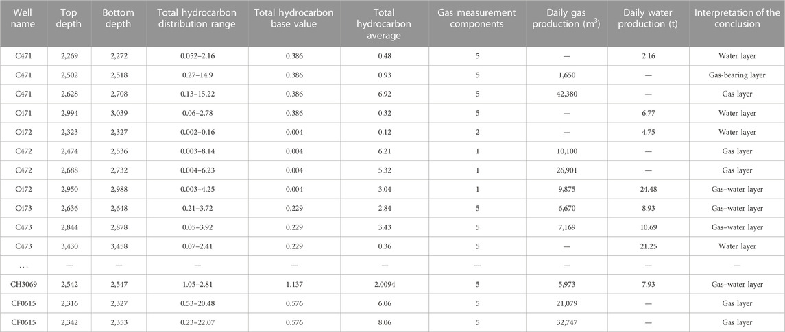
TABLE 1. Oil test, production data, and gas survey data from the study area.
The hydrocarbon humidity value calculation formula is
where C1 is the dry gas and C2–5 represent the wet gas. Wh is the humidity, which can be used to determine the hydrocarbon type (oil or gas).
The logging response characteristics of the main fluids in the area were analyzed and summarized based on the oil testing conclusion data and logging curves from five wells (Tables 2, 3).
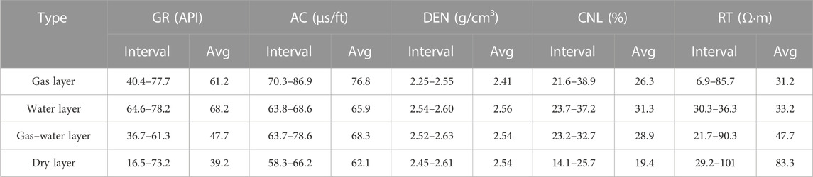
TABLE 2. Response characteristics of caved-fracture fluid logging.
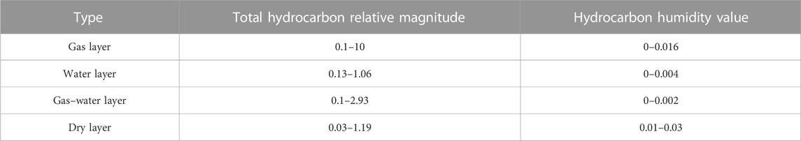
TABLE 3. Response characteristics of caved-fracture fluid mud logging.
Based on the analysis and summary of the caved-fracture fluid logging response characteristics in the study area in Tables 2, 3, according to the data of 73 oil test intervals of 24 wells in the C471 well area, the corresponding logging parameters were selected as QL-RT, DEN-AC, CNL-GR, and RD/RT-RI cross-plots (Figure 1) to identify the caved-fracture fluid.
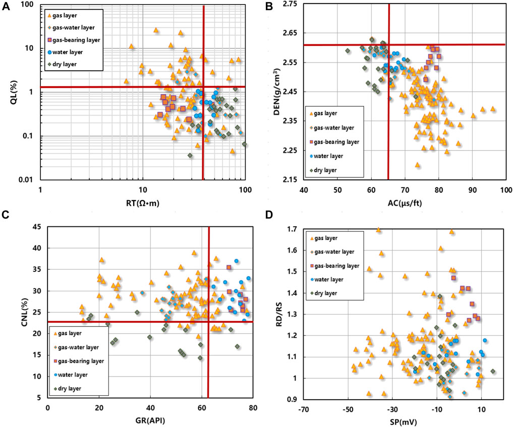
FIGURE 1. Cross-plot of logging parameters: (A) RT and QL; (B) AC and DEN; (C) GR and CNL; (D) SP and RD/RS.
Based on Figures 1A–D, it can be observed that the gas layer, gas-bearing layer, and water layer exhibit low resistivity, while the dry layer displays high resistivity. The gas layer has the characteristics of high acoustic wave and low density, which is different from other fluid characteristics. The density log value of the dry layer is the highest, followed by the gas–water layer and the water layer. According to the neutron-gamma logging response, the dry layer presents the characteristics of low–medium gamma and low neutron logging value, the neutron logging value is significantly lower than that of the gas layer, and the neutron logging value of the water layer is slightly larger than that of the gas layer. Generally, conventional well logging curves such as RT, CNL, DEN, AC, and QL (full hydrocarbon) curves are highly sensitive to fluid properties.
Although the cross-plot method can reflect the properties of formation fluids to a certain extent, from the cross-plot, it can be observed that the cross-plot method is effective in distinguishing between dry layers and fluid reservoirs. However, it faces challenges in effectively differentiating gas layers, gas–water layers, and water layers. It shows that the single conventional cross-plot has a poor overall effect on the identification of caved-fracture fluids and cannot make full use of logging curves reflecting fluid properties and express the semantic level stratigraphic information contained in the logging curve.
3 Model principle and construction
3.1 Stacked generalization principle
Stacked generalization (David, 1992), as a typical learning method in ensemble learning (Lü et al., 2019), uses a certain learner to integrate the classification results of different base learners. The stacked generalization model can increase the nonlinear ability of the model by increasing the number of layers, but at the same time, it will also lead to the phenomenon of model overfitting. Therefore, the general stacked generalization model is a two-layer structure (Niyogisubizo et al., 2022). The stacked generalization model ensemble machine learning algorithm models with better identification effects, such as decision trees, nearest neighbors, and support vector machine algorithms. It makes full use of the different characteristics of different algorithms and then uses a new meta-learner to combine the prediction results of individual base learners to finally complete the prediction of the task results. The algorithm implementation process is illustrated in Figure 2. First, the dataset is divided into multiple subsets, which serve as inputs for the basic learners. Each basic learner generates a prediction result based on its corresponding subset. The outputs of all the basic learners are then used as inputs for the meta-learner, which produces the final prediction result. By stacking and generalizing the outputs of multiple base learners, the overall task’s prediction accuracy is improved.
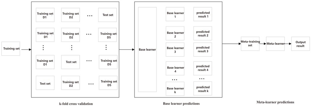
FIGURE 2. Stacked generalization process.
In order to prevent the meta-learner from directly learning the training set of the base learner, which causes too much risk of overfitting, the learning of the base learner is carried out by means of cross-validation (Geisser, 1975). The original training set D is randomly divided into k sets
Considering the diverse principles underlying the base learners and their varying interpretations of the data space dimensions in well logging information (Zhou H et al., 2021), classic algorithms such as the SVM, KNN, decision trees, and stochastic gradient descent classification method have been widely used in the field of machine learning for many years and have been extensively validated in practical applications. These algorithms have broad application domains and are supported by a rich body of research, demonstrating their ability to achieve robust performance in various problem domains (Wu et al., 2017; Zhou X et al., 2021; Jung and Kim, 2023; Pałczyński et al., 2023). Therefore, in this article, they are used as the base learner, and the fully connected neural network is used as the meta-learner (detailed in the subsequent section). The pseudocode is shown in Table 4.
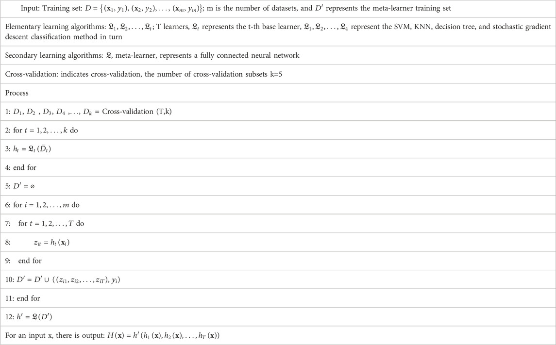
TABLE 4. Schematic diagram of the implementation steps of the stacked generalization algorithm.
Among them,
3.2 Model construction
Based on the introduction provided in the previous section, the SVM, KNN, decision tree, and stochastic gradient descent classification method with different mathematical principles are used as the base learners, and the fully connected neural network commonly used in deep learning is used as the meta-learner to control the final output. Among them, the fully connected neural network is also called multilayer perceptron, which is a kind of artificial neural network with forward feedback (Du et al., 2020), known as the deep feedforward network. A feedforward neural network includes an input layer, a hidden layer, and an output layer. The input layer mainly associates the feature information with the input nodes, transmits information for the hidden nodes in the next step, and provides data support for the calculation in the next step. The hidden layer is a node layer that further processes the feature information, calculates the data transmitted by the input node, and transmits the calculated information to the output node to improve the nonlinear ability of the model. The output layer is the last link in the transmission of information, which further calculates the data and transmits information to the outside of the network (Figure 3).
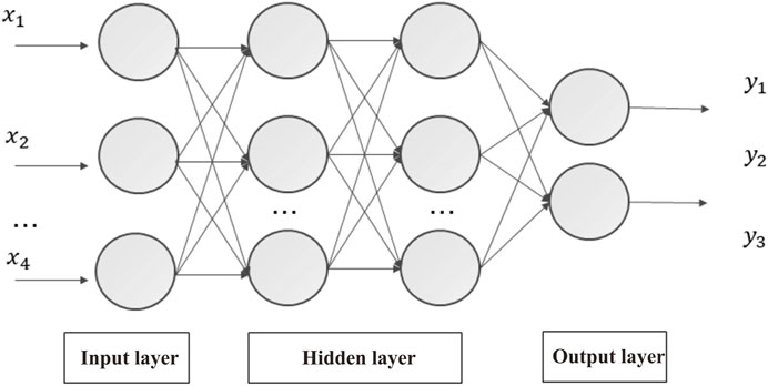
FIGURE 3. Meta-learner model structure diagram.
In the forward propagation stage, it can be seen that the input layers x1, x2.xn form the X vector. Therefore, the hidden layer neurons are activated by the hyperbolic function tanh to obtain the output value of this layer:
where aj represents the output value of the hidden layer neuron, tanh represents the hidden layer activation function, gj represents the input weighted sum of the j-th hidden layer neuron node, n represents the number of neurons in the input layer, i represents the subscript of the input layer neuron, j represents the subscript of the hidden layer neuron, and wij is the weight of the hidden layer neuron j.
Similarly, the output value of the output layer neuron is activated by the normalized exponential function softmax, which can be expressed as
where y (ak) represents the output value of the hidden layer neuron, softmax represents the activation function of the output layer, m is the number of neurons in the hidden layer, wjk is the weight of the output layer neuron k, and xjk represents the output value of the neurons in the hidden layer, which is equal to the input value of the neurons in the output layer.
Let
From the definition of the softmax function, it can be known that
where p represents the number of neurons in the output layer.
The loss function can be expressed as
In the backpropagation stage, when the loss function is passed from the output layer to the input layer, the stochastic gradient descent algorithm (SGD) is used as the optimizer to iteratively adjust the model weight. This method is the most basic iterative algorithm for optimizing neural networks at present, and it is simple and easy to implement (Li et al., 2022).
The gradient is also the partial derivative of the loss function L with respect to the weight w, and the calculation based on the chain rule can be expressed as
The weight of the updated output layer can be obtained from the aforementioned formula, which is expressed as
where η represents the model learning rate that controls the update speed of the parameters.
4 Model parameter selection
4.1 Data normalization
Conventional well logging curves RT, CNL, DEN, AC, and QL are used as sample points, respectively, where QL can be calculated from the gas measurement data. According to the oil test data, 121 oil test intervals of 38 exploration wells were selected, and the corresponding fluid-sensitive logging parameters (deep lateral resistivity (RT), neutron (CNL), acoustic time difference (AC), formation density (DEN), and total hydrocarbon index (QL)) were used as the input data of the basic learner. The training dataset for this study consists of 100 samples, while the testing dataset comprises 26 samples. Among these, there are 76 training samples and 18 prediction samples for gas reservoirs. For water reservoirs, there are eight training samples and three prediction samples. Finally, for the gas–water layers, there are 16 training samples and 5 prediction samples. The distribution of sample data is shown in Table 5.

TABLE 5. Caved-fracture fluid sample data selection.
Based on the earlier discussion, where the cross-plot method demonstrated effective identification of dry formations, we will not specifically focus on the identification of dry formations in this study. The fluid data are mainly divided into the gas layer, water layer, and gas–water layer. The label is set to 0 for the water layer, 1 for the gas layer, and 2 for the same layer of gas–water.
The dimension and order of magnitude of different logging information are different. To eliminate the influence of unit and scale difference between logging information, it is necessary to normalize the features and normalize the input logging response feature data. The formula can be expressed as
For nonlinear logarithmic characteristic curves, such as RT curves, logarithmic transformation should be performed before entering the model:
In the formula,
4.2 Base learner parameter selection
After data standardization, the dataset was randomly divided into the training set and test set in the ratio of 8:2, and the training set was further divided into the sub-training set and sub-validation set using the five-fold cross-validation method. Using the sub-training set to train the model and the verification set to verify the training effect, the size of the model parameters is adjusted based on the effect of the verification. This process helps in selecting the optimal parameters for the basic learner. Stochastic gradient descent, KNN algorithm, decision tree algorithm, and support vector machine algorithm were selected as the basic learners, and different parameters in the algorithm were set. The relationship between different parameters of the experiment and the accuracy rate is shown in Figure 4.
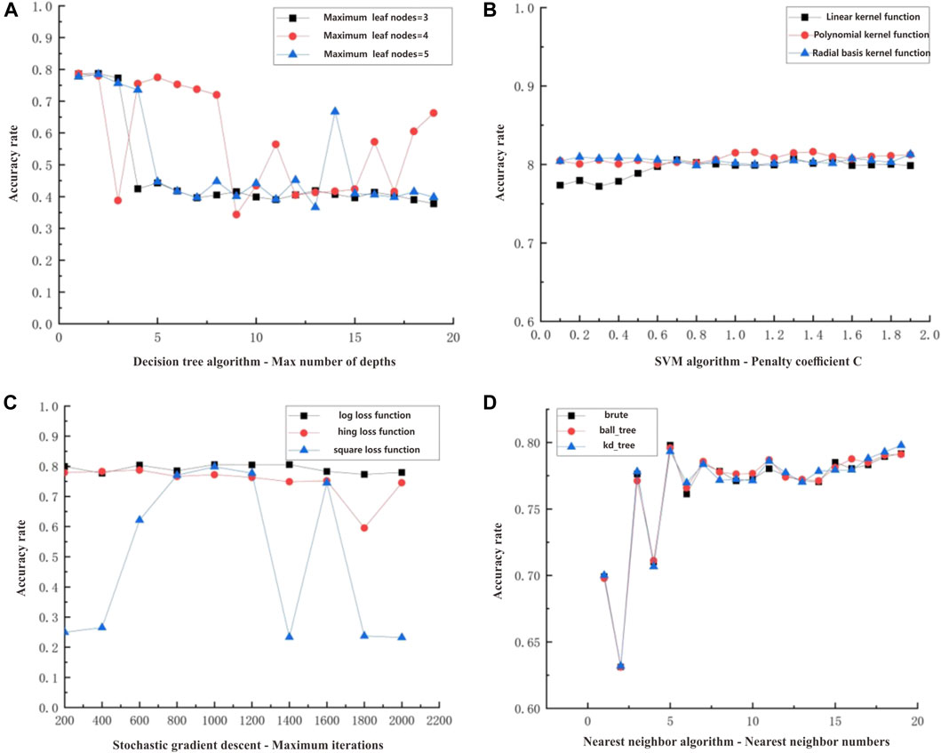
FIGURE 4. Relationship between different base learner parameters and accuracy rate: (A) maximum depth and accuracy; (B) regularization coefficient and accuracy; (C) number of iterations and accuracy; (D) nearest neighbor numbers and accuracy.
Among them, the maximum depth and the maximum number of leaf nodes are used as the decision parameters of the decision tree. Since the number of features is selected as 5, the maximum leaf child nodes of the decision tree are set to 3, 4, and 5. The larger the maximum depth of the decision tree is, the more the tree is split, the ability of the model to capture the nonlinearity of the data is enhanced, the probability of the model overfitting is increased, and the generalization ability of the model is worse. It can be seen from Figure 4A that with the increase in the maximum depth of the decision tree, the accuracy of the model shows a fluctuating trend. When the maximum depth is 5 and the maximum number of child nodes is 4, the model accuracy is the highest, which is 79.8%.
The SVM algorithm completes the classification by maximizing the classification interface and finding a hyperplane to separate the classification targets as much as possible. When using SVM to identify fluids, it is necessary to pay attention to the penalty term coefficient C and the corresponding kernel function. Increasing the penalty coefficient C in a model strengthens its ability to constrain and suppress the parameters, which can lead to a higher degree of regularization. However, if the penalty coefficient C is set to an excessively large value, it can result in excessive parameter suppression and potentially cause underfitting. Kernel functions are generally used for higher-dimensional target tasks and can also provide models with different nonlinear capabilities. It can be seen from Figure 4B that in the SVM classification algorithm, the accuracy of the results using the polynomial and radial basis kernel functions is higher than that of the linear kernel function, and the accuracy of the polynomial kernel function is slightly higher than that of the radial basis kernel function. When the penalty term coefficient C is 1.1 and the kernel function is a polynomial optimizer, the model has the best accuracy of 81.5%.
It can be seen from Figure 4C that the stochastic gradient descent method is affected by the maximum number of iterations and the loss function. The log, hing, and square loss functions are selected as experimental comparisons. When the loss function is log loss, the stochastic gradient descent method evolves into a logistic regression algorithm with fast convergence and stable overall accuracy, with the highest accuracy reaching 81.2%. Other loss functions are more volatile and unstable, among which the square loss function has the most violent fluctuation.
As seen from Figure 4D, the KNN algorithm is affected by the number of nearest neighbors and the construction method of the tree. The construction method of the tree is divided into brute, kd-tree, and ball-tree. It can be found that the construction method of the tree has no obvious influence on the algorithm. When experimenting on the number of nearest neighbors, it is found that the number of nearest neighbor algorithms has a significant impact on the generalization effect of the model. When the number of nearest neighbors is 5, the highest accuracy is 79.7%. When the number of nearest neighbors is 15–20, the accuracy rate is not much different. When the number of nearest neighbors is larger, the model is more prone to overfitting, so the optimal number of nearest neighbors is 5.
4.3 Meta-learning model parameter optimization
The initial learning rate of the meta-learner is set to 0.001. Considering that there are too few data sample points, the model is prone to overfitting, and the regularization parameter penalty factor is set to 0.0005. The input layer is the secondary training set constructed by the output of the four basic learners after cross-validation training. Two hidden layers are set in the middle of the meta-learner, the number of neurons is set to 128 and 128, respectively, and the number of output neurons is set to 3. The learning rate decay factor is 0.8. The meta-learner is trained for 10,000 rounds, and the training loss and test loss are reduced to 0.04 and 0.03, respectively (Figure 5). It can be seen from the curve that the training set loss and the validation set loss have a stable and consistent downward trend, and there is no overfitting phenomenon.
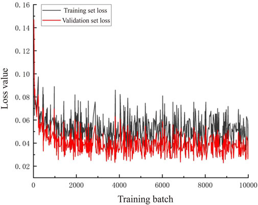
FIGURE 5. Meta-learner training time loss trend chart.
The accuracy rate obtained by inferring the test set with the meta-learner model is used as the evaluation index, and the calculation method of the accuracy rate is as follows:
where P is the accuracy rate and TP is the number of positive samples where the sample itself is positive. The model also predicts the number of positive samples, and FP is the number of negative samples that are predicted to be positive samples.
The hyperparameter training batch, the number of intermediate hidden layers, the learning rate, and the regularization parameters in the experiment are modified. Based on the experimental method, the optimal parameters of the fully connected neural network model were selected, the accuracy of the model test set was used as the measurement index, and judging whether the model is overfitting is supplemented by the accuracy of the training set. The training batch-accuracy, learning rate-accuracy, number of hidden layers-accuracy, and regularization coefficient-accuracy graphs are made, respectively (Figures 6A–D).
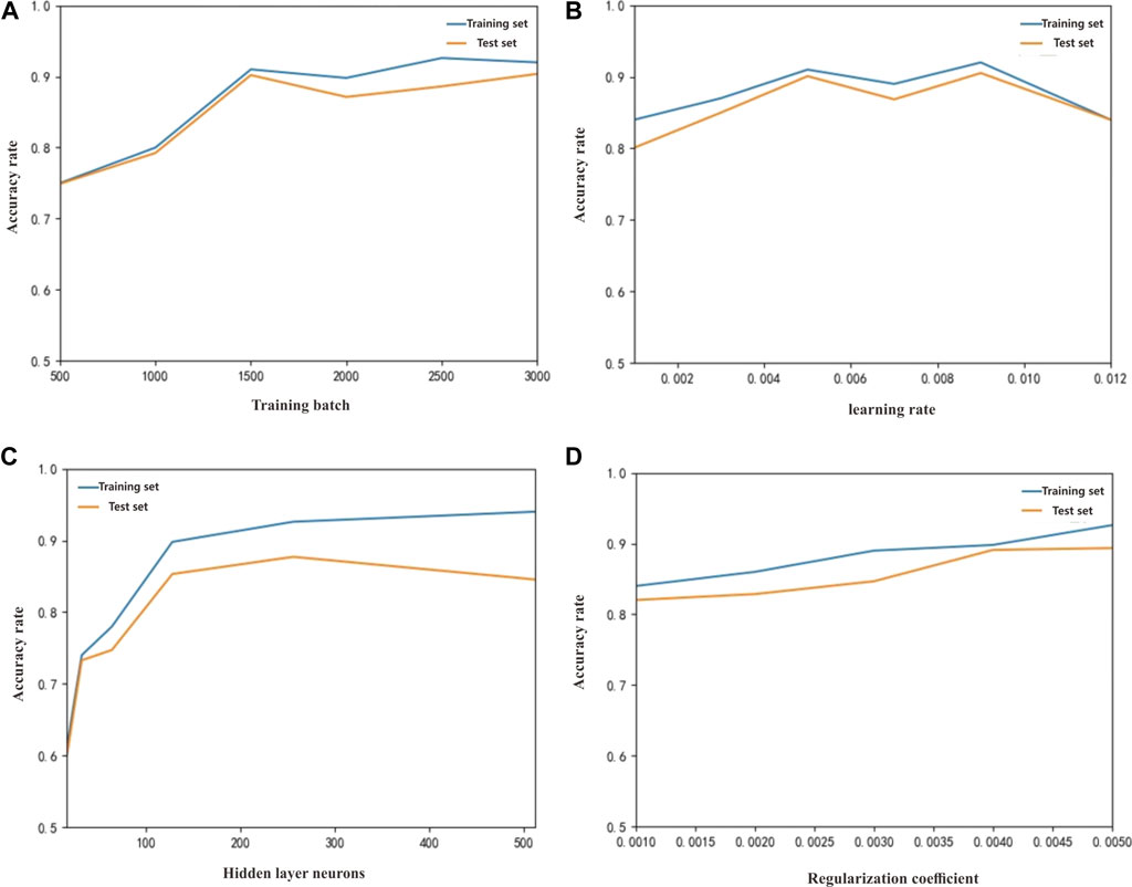
FIGURE 6. Relationship between different meta-learning parameters and accuracy rate: (A) training batch and accuracy; (B) learning rate and accuracy; (C) hidden layer neural and accuracy; (D) regularization coefficient and accuracy.
When the other parameters are fixed at a specific value, the training batches are set in the range of 500–3,000, with an interval of 500 for each training iteration (Figure 6A). It is found that the training batch tends to be stable from 2,500 to 3,000, and the accuracy trend of the training and test sets are consistent, with no overfitting. At this time, the batch is 2,500 and has the best accuracy. When the model learning rate is too small, the network model is prone to fall into local optimum, and when the model is too large, it is not stable enough and lacks robustness. It can be seen from Figure 6B that when the learning rate is 0.009, the model training accuracy is high. When the number of neurons in the hidden layer is small, the model is prone to underfitting and lacks nonlinear ability. As the number of neurons increases, the nonlinear ability of the model increases. When the number of neurons is 512, the training accuracy increases and the test accuracy decreases significantly, and overfitting occurs at this time (Figure 6C). Therefore, the number of neurons should be 256 for the best accuracy. As the regularization coefficient increases, the penalty for the parameters is larger, and the ability to suppress overfitting is stronger. When the regularization coefficient is 0.004, the model test accuracy is the highest (Figure 6D).
5 Field examples
Based on Section 3.2, model construction, meta-learner parameter selection (Table 6) is used to construct the model. Partial training sample data are shown in Table 7. The specific flow chart of the model is shown in Figure 7, which predicts the results of the fluid data of Carboniferous reservoirs in the study area.
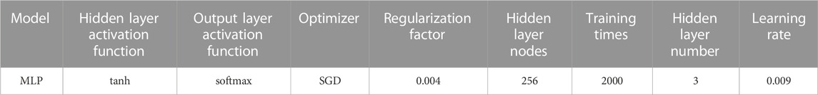
TABLE 6. Corresponding parameters of the caved-fracture fluid prediction model.
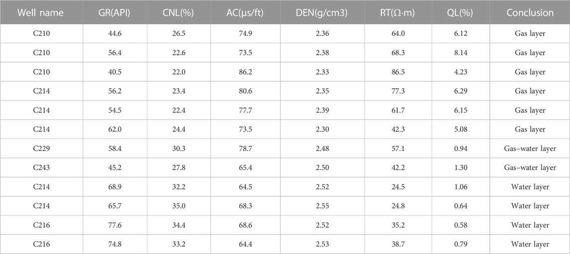
TABLE 7. Partial training sample data.
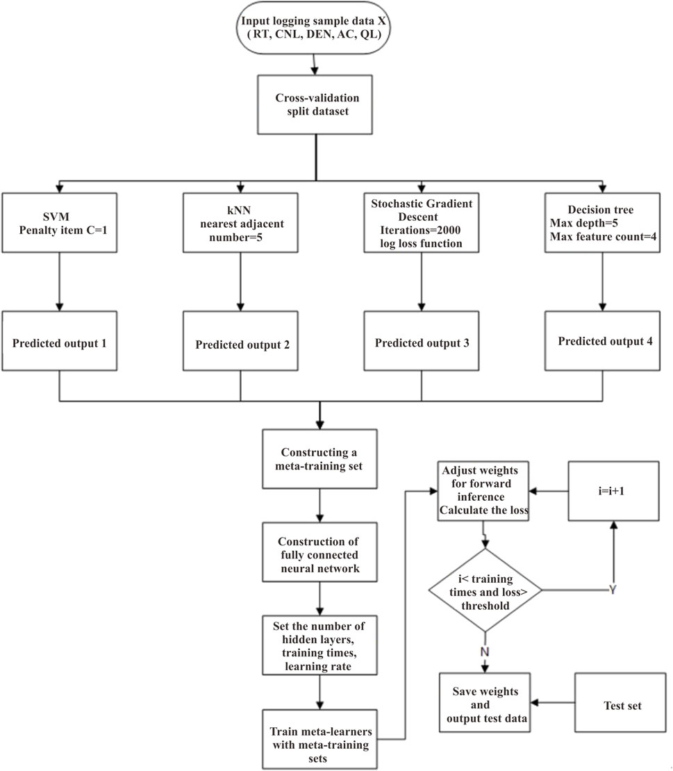
FIGURE 7. Flowchart of stacking generalization method application.
Table 8 demonstrates that the interpreted conclusion is generally consistent with the oil test conclusion. The highest recognition rate for gas layers in the training samples is 98.7%, while in the test set, it reaches 88.8%. Graphing Table 8, it can be seen that the stacked generalization model identifies fluids more effectively than the single model (Figure 8).
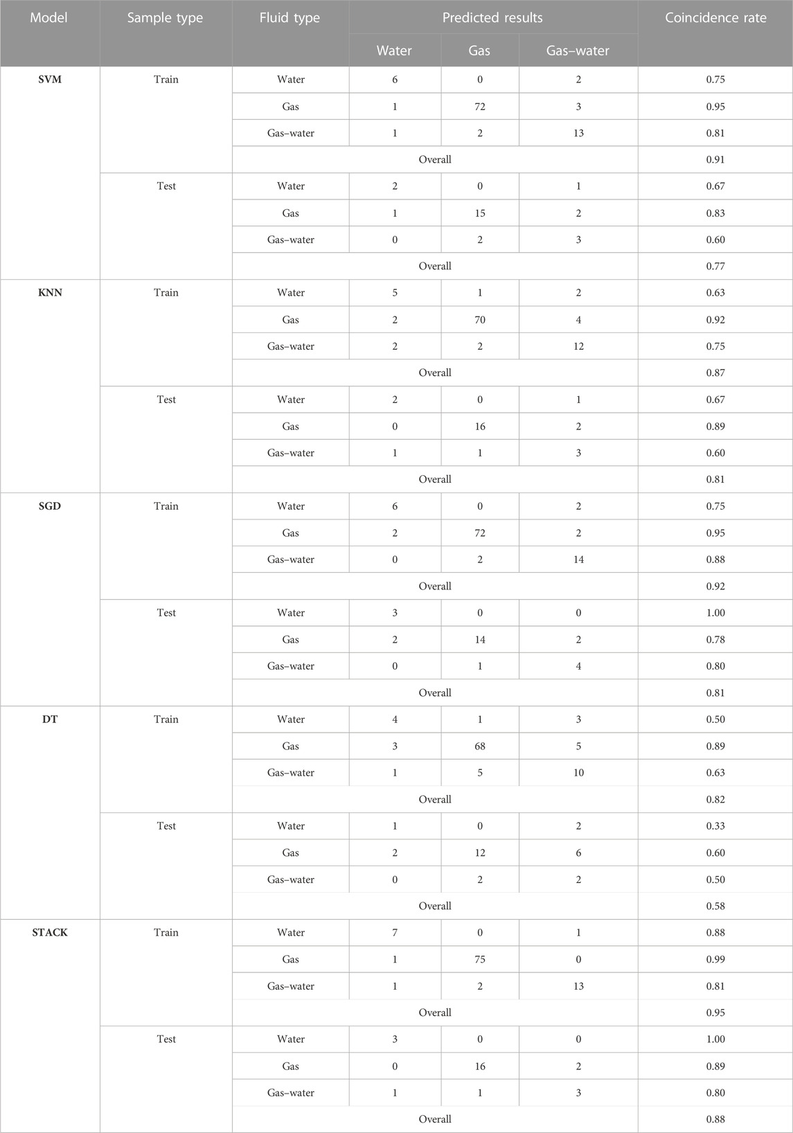
TABLE 8. Results of caved-fracture fluid identification for different models.

FIGURE 8. Graph of fluid identification accuracy of different models: (A) accuracy of training sample; (B) accuracy of testing sample.
The stacking generalization model was used to explain the processing and interpretation of the oil test interval of well CF6 in the study area (Figure 9). For the fluids in different well areas, the stacking generalization fusion model is used to identify the fluids, and the new and old perforated wells are combined with the logging method to identify the fluids. Oil test section: 2,749–2,762 m, daily gas production is 52,157 cubic meters, and the daily water production is 0t. Since 0 in the model output means that the model has no reasoning, the model output is increased by 1, and the outputs 1, 2, and 3 represent the water layer, gas–water layer, and gas layer, respectively. In the 2,749–2,754 m section, the density log response value decreased, the neutron log response value increased, the resistivity showed a downward trend, and the model inferred that it was a gas layer. In the 2,756–2,762.3 m section, the density logging response value decreased, the neutron logging response value increased, resistivity showed a downward trend, and the acoustic logging response value was inferred as a gas layer by the model. In the 2,764–2,771 m section, the density shows a downward trend, the acoustic wave value increases accordingly, the neutron value logging response value increases, and the resistivity shows a gentle downward trend. The model of 2,764–2,771 m is inferred as a water layer. The model interpretation corresponds to the gas layer and the water layer, respectively, and also corresponds to the gas measurement data. From the oil test interpretation conclusion and the model interpretation conclusion, it can be seen that the model interpretation conclusion is roughly consistent with the oil test conclusion.
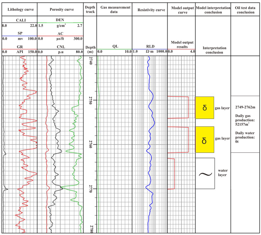
FIGURE 9. Interpretation results of the stacking generalization method in the oil test interval (2,749–2,762 m) of well CheF6.
The stacking generalization method was also used for fluid identification in the CH21100 well area. Fluid identification was performed based on new and old perforated wells combined with logging methods, and a recommended well section was suggested. The mud logging shows that the gas measurement section, which has a thickness of 20 m and QL between 2.93% and 8.348%, was interpreted as a gas layer (Figure 10). Oil test section: 1,202–1,222 m, daily gas production is 62,852 cubic meters; 1,240–1,275 m, daily gas production is 16,553 cubic meters, and the daily water production is 12.4t. The interpretation of the model suggests that the gas layers are located in the 1,179–1,183 m, 1,203–1,209 m, and 1,210–1,237 m sections, while the gas–water layer is in the 1,244–1,258 m section. These results are consistent with the comprehensive mud logging interpretation and oil testing conclusions.
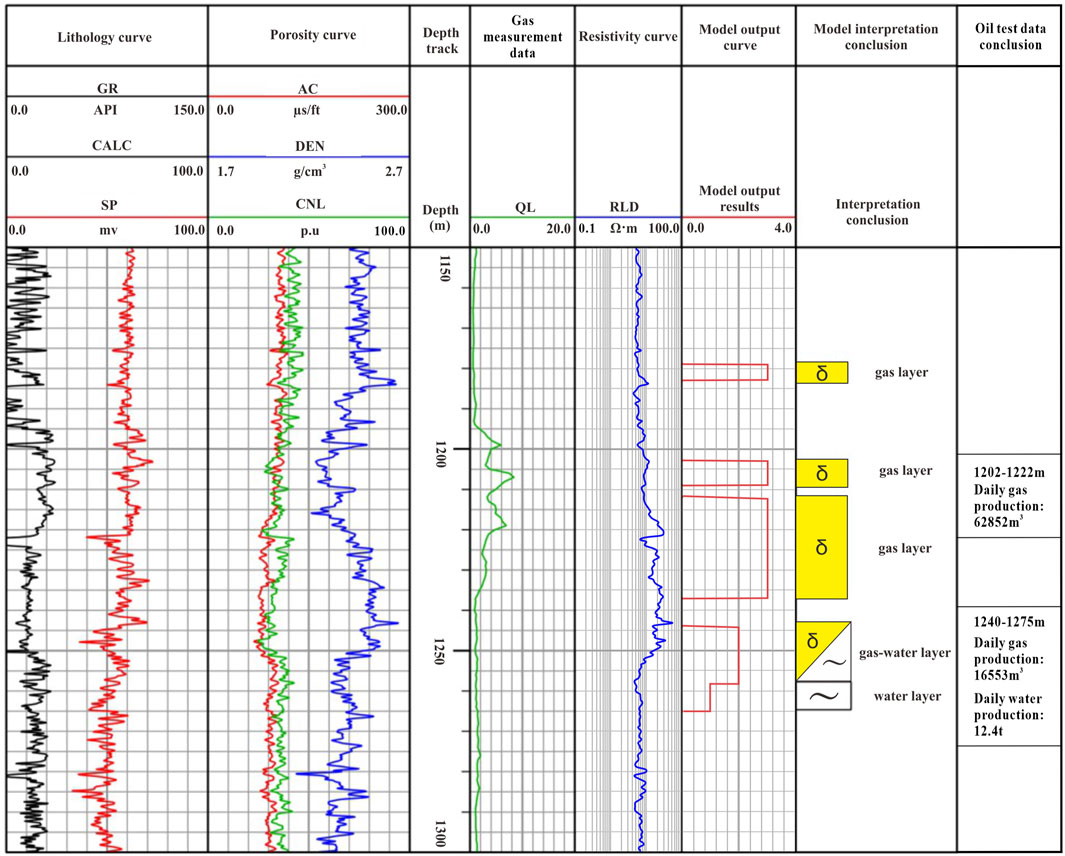
FIGURE 10. Comprehensive interpretation results of logging and logging in well CH21100.
6 Conclusion
This paper proposes a classification method based on a stacked generalization model to identify caved-fracture fluid properties.
1) Compared to cross-plot and single machine learning discriminative models, the fluid identification method based on stacked generalization models yields superior results and enhances the effectiveness of fluid identification in the caved-fracture reservoirs.
2) The fusion algorithm based on the stacked generalization model can obtain the global optimal parameters through two modes: cascade learning and model fusion, which makes up for the shortcomings of common machine algorithms such as insufficient generalization ability and long training time.
3) The SVM, KNN, stochastic gradient descent, and decision tree algorithm were used as the base learners, a fully connected neural network was used as the meta-learner, the classification loss was used as the cost objective function, the gradient descent method was used to optimize the model parameters, and a stacking generalization model was built for recognition research of the fluid properties of the oil interval in the regional test. The results show that the recognition accuracy rate of the model based on stacking generalization reaches 88%.
4) In practical applications, the lack of coring data, similar mineral composition, and structure of certain rock types can result in errors in the model fluid identification of boundary intervals. To address this deficiency, logging data can be combined to complement the analysis.
Data availability statement
The original contributions presented in the study are included in the article/Supplementary Material; further inquiries can be directed to the corresponding author.
Author contributions
JZ: conceptualization, methodology, and writing—review and editing. ZL: formal analysis, methodology, and writing—original draft preparation. QL: investigation, resources, and validation. WC: supervision and investigation. ZW: visualization and data curation. All authors contributed to the article and approved the submitted version.
Funding
This paper was supported by State Key Laboratory of Oil and Gas Reservoir Geology and Exploitation, Southwest Petroleum University. The views expressed are the authors' alone.
Conflict of interest
Author QL was employed by CNPC.
The authors declare that this study received funding from the CNPC-SWPU Innovation Consortium Project (2020CX010204). The funder had the following involvement: study design, data collection and analysis.
The remaining authors declare that the research was conducted in the absence of any commercial or financial relationships that could be construed as a potential conflict of interest.
Publisher’s note
All claims expressed in this article are solely those of the authors and do not necessarily represent those of their affiliated organizations, or those of the publisher, the editors, and the reviewers. Any product that may be evaluated in this article, or claim that may be made by its manufacturer, is not guaranteed or endorsed by the publisher.
References
Ahmed, N., Khalid, P., Shafi, H. M. B., and Connolly, P. (2017). DHI evaluation by combining rock physics simulation and statistical techniques for fluid identification of Cambrian-to-Cretaceous clastic reservoirs in Pakistan. Acta geophys. 65, 991–1007. doi:10.1007/s11600-017-0070-5
Bai, Z., Tan, M., Shi, Y., Guan, X., Wu, H., and Huang, Y. (2022). Log interpretation method of resistivity low-contrast oil pays in Chang 8 tight sandstone of Huan Xian area, Ordos Basin by support vector machine. Sci. Rep. 12 (1), 1046. doi:10.1038/s41598-022-04962-0
Bian, H., Pan, B., and Wang, F. (2013). Volcanic reservoirs fluid identification by neural network based on shear wave log data. Well Logging Technol. 37 (03), 264–268. doi:10.16489/j.issn.1004-1338.2013.03.015
Cai, Z. (2021). Research on lithologic identification based on bayesian probability model. Chang' an University.
Cao, M., Gong, W., and Gao, Z. (2022). Research on lithology identification based on stacking integrated learning. Comput. Technol. Dev. 32 (7), 161–166. doi:10.3969/j.issn.1673-629X.2022.07.028
Chen, G., Yin, X., Li, J., Gao, Y., and Gao, M. (2017). Derivation of human-induced pluripotent stem cells in chemically defined medium. Special Oil Gas Reserv. 24 (05), 131–137. doi:10.1007/978-1-4939-6921-0_9
Dai, S. (2018). Volcanic lithology and reservoir identification based elastic wave characteristics analysis in Yingcheng Formation, Xujiaweizi Depression. Oil Geophys. Prospect. 53 (01), 122–128+8. doi:10.13810/j.cnki.issn.1000-7210.2018.01.015
David, H. (1992). Stacked generalization. Neural Netw. 5 (02), 241–259. doi:10.1016/s0893-6080(05)80023-1
Du, X., Fan, T., Dong, C., Nie, Y., Fan, H., and Guo, B. (2020). Characterization of thin sand reservoirs based on a multi-layer perceptron deep neural network. Oil Geophys. Prospect. 55 (06), 1178–1187+1159. doi:10.13810/j.cnki.issn.1000-7210.2020.06.002
Geisser, S. (1975). The predictive sample reuse method with applications. J. Am. Stat. Assoc. 70, 320–328. doi:10.1080/01621459.1975.10479865
He, D., Chen, X., and Guan, J. (2010). Characteristics and exploration potential of Carboniferous hydrocarbon plays in Junggar Basin. Acta Pet. Sin. 31 (01), 1–11. doi:10.7623/syxb201001001
He, M., Gu, H., and Xue, J. (2022). Log interpretation for lithofacies classification with a robust learning model using stacked generalization. J. Petroleum Sci. Eng. 214, 110541. doi:10.1016/j.petrol.2022.110541
Jia, J., Li, C., Wang, L., and Zhao, N. (2018). Experimental study on identification of influencing factors of igneous gas and water layer by longitudinal and shear wave velocities. Reserv. Eval. Dev. 8 (05), 8–13. doi:10.13809/j.cnki.cn32-1825/te.2018.05.002
Jiang, C., Dai, S., Wu, J., Liu, Y., and Zhou, E. (2014). Elastic parameter tests and characteristics analysis of volcanic rocks in Yingcheng Formation, Northern Songliao Basin. Oil Geophys. Prospect. 49 (05), 916–924+820. doi:10.13810/j.cnki.issn.1000-7210.2014.05.042
Jung, T., and Kim, J. (2023). A new support vector machine for categorical features. Expert Syst. Appl. 229, 120449. doi:10.1016/j.eswa.2023.120449
Kumar, T., Seelam, N. K., and Rao, G. S. (2022). Lithology prediction from well log data using machine learning techniques: a case study from talcher coalfield, eastern India. J. Appl. Geophys. 199, 104605. doi:10.1016/j.jappgeo.2022.104605
Li, M., Lai, G., Chang, Y., Feng, Z., Cao, K., Song, C., et al. (2022). Research progress of Nedd4L in cardiovascular diseases. Inf. Technol. Inf. 8 (03), 206–209. doi:10.1038/s41420-022-01017-1
Li, Y., and Anderson-Sprecher, R. (2006). Facies identification from well logs: a comparison of discriminant analysis and naïve bayes classifier. J. Petroleum Sci. Eng. 53, 149–157. doi:10.1016/j.petrol.2006.06.001
Lü, P., Yu, W., Wang, X., Ji, C., and Zhou, X. (2019). Stacked generalization of Heterogeneous classifiers and its application in toxic comments detection. Acta Electron. Sin. 47 (10), 2228–2234. doi:10.3969/j.issn.0372-2112.2019.10.026
Maiti, S., Tiwari, R. K., and Kümpel, H. J. (2007). Neural network modelling and classification of lithofacies using well log data: a case study from ktb borehole site. Geophys. J. Int. 169 (02), 733–746. doi:10.1111/j.1365-246x.2007.03342.x
Niyogisubizo, J., Liao, L., Nziyumva, E., Murwanashyaka, E., and Nshimyumukiza, P. C. (2022). Predicting student's dropout in university classes using two-layer ensemble machine learning approach: a novel stacked generalization. Comput. Educ. Artif. Intell. 3, 100066. doi:10.1016/j.caeai.2022.100066
Pałczyński, K., Czyżewska, M., and Talaśka, T. (2023). Fuzzy Gaussian decision tree. J. Comput. Appl. Math. 425, 115038. doi:10.1016/j.cam.2022.115038
Qin, M., Hu, X., Liang, Y., Yuan, W., and Yang, D. (2021). Using Stacking model fusion to identify fluid in high-temperature and high-pressure reservoir. Oil Geophys. Prospect. 56 (02), 364–371+214-215. doi:10.13810/j.cnki.issn.1000-7210.2021.02.019
Wang, S., Xu, Z., Liu, H., Wang, Z., and Shi, L. (2004). The advanced k-nearest neighborhood method used in the recognition of lithology. Prog. Geophys. (02), 478–480.
Wu, X., Wang, S., and Zhang, Y. (2017). Survey on theory and application of K-nearest neighbor algorithm. Comput. Eng. Appl. 53 (21), 1–7. doi:10.3778/j.issn.1002-8331.1707-0202
Zhang, L., Pan, B., Shan, G., He, L., Yang, D. l., Yan, Z. S., et al. (2008). Method for identifying fluid property in volcanite reservoir. Oil Geophys. Prospect. 43 (06), 728–732-612+742. doi:10.3321/j.issn:1000-7210.2008.06.020
Zhao, J., Lu, Y., Li, Z., and Liu, J. (2015). Application of density clustering based K-nearest neighbor method for fluid identification. J. China Univ. Petroleum Ed. Nat. Sci. 39 (5), 65–71. doi:10.3969/j.issn.1673-5005.2015.05.009
Zhou, B., Han, C., and Guo, T. (2021). Convergence of stochastic gradient descent in deep neural network. Acta Math. Appl. Sin. 37 (01), 126–136. doi:10.1007/s10255-021-0991-2
Zhou, H., Zhang, C., Zhang, X., Wu, Z., and Ma, Q. (2021). Lithology identification method of carbonate reservoir based on capsule network. Nat. Gas. Geosci. 32 (05), 685–694. doi:10.11764/j.issn.1672-1926.2020.11.018
Zhou, J. (2021). Research on application of deep learning in lithology recognition of oil and gas reservoir. Lanzhou University of Technology.
Zhou, X., Li, Y., Song, X., Jin, L., and Wang, X. (2023). Thin reservoir identification based on logging interpretation by using the support vector machine method. Energies 16 (4), 1638. doi:10.3390/en16041638
Keywords: caved-fracture reservoir, machine learning, fluid identification, logging, stacked generalization
Citation: Zhao J, Lin Z, Lai Q, Chen W and Wu Z (2023) A fluid identification method for caved-fracture reservoirs based on the stacking model. Front. Earth Sci. 11:1216222. doi: 10.3389/feart.2023.1216222
Received: 03 May 2023; Accepted: 24 July 2023;
Published: 10 August 2023.
Edited by:
Qiaomu Qi, Chengdu University of Technology, ChinaReviewed by:
Jun Wang, Chengdu University of Technology, ChinaFuqiang Lai, Chongqing University of Science and Technology, China
Copyright © 2023 Zhao, Lin, Lai, Chen and Wu. This is an open-access article distributed under the terms of the Creative Commons Attribution License (CC BY). The use, distribution or reproduction in other forums is permitted, provided the original author(s) and the copyright owner(s) are credited and that the original publication in this journal is cited, in accordance with accepted academic practice. No use, distribution or reproduction is permitted which does not comply with these terms.
*Correspondence: Weifeng Chen, c3dwdWN3ZkAxMjYuY29t