 Grace L. Brown
 Ben W. Brock
- Department of Geography and Environmental Sciences, Northumbria University, Newcastle upon Tyne, United Kingdom
The cryosphere plays an important role in the global carbon cycle, but few studies have examined carbon fluxes specifically on debris-covered glaciers. To improve understanding of the magnitude and variability of the atmospheric carbon flux in supraglacial debris, and its environmental controls, near-surface CO2 fluxes and meteorological variables were monitored over thick (0.23 m) and thin (0.04 m) debris at Miage Glacier, European Alps, over two ablation seasons, using an eddy covariance system. The CO2 flux alternates between downward and upward orientation in the day and night, respectively, and is dominated by uptake of CO2 in thick debris (mean flux = 1.58 g CO2 m−2 d−1), whereas flux magnitude is smaller and near net zero on thin debris (mean flux = −0.06 g CO2 m−2 d−1). These values infer a potential drawdown of >150 t CO2 km−2 over an ablation season, and >500 t CO2 (0.5 Gg CO2) for the whole debris-covered zone. The strong correlation of daytime CO2 flux magnitude with debris surface temperature suggests that atmospheric CO2 is consumed in hydrolysis and carbonation reactions at sediment-water interfaces in debris. Incoming shortwave radiation is key in heating debris, generating dilute meltwater, and providing energy for chemical reactions. CO2 drawdown on thin debris increases by an order of magnitude on days following frost events, implying that frost shattering generates fresh reactive sediment, which is rapidly chemically weathered with the onset of ice melting. Net CO2 release in the night, and in the daytime when debris surface temperature is below 7°C, is likely due to respiration by debris microorganisms. The combination of dilute meltwater, high temperature, and reactive mineral surfaces open to the atmosphere, makes supraglacial debris an ideal environment for rock chemical weathering. Debris-covered glaciers could be important to local and regional carbon cycling, and measurement of CO2 fluxes and controlling processes at other sites is warranted.
1 Introduction
The global extent of supraglacial rock debris has been estimated as 29,183 km2, equivalent to about 7% of total mountain glacier area, with prominent cover in High Mountain Asia, the Andes, Alaska, and the Arctic (Herreid and Pellicciotti, 2020). Debris-covered glaciers (DCGs), defined as having continuous debris cover across a large part of their ablation zone (Kirkbride, 2011) are present in most of the world’s glacierised mountain ranges, and their global area is expected to increase as climate warms (Scherler et al., 2018; Tielidze et al., 2020). Recent studies have demonstrated the distinctive influence of supraglacial debris on glacier mass balance and climatic response (Scherler et al., 2011; Fyffe et al., 2014; Rowan et al., 2015; Nicholson et al., 2021; Rounce et al., 2021; Wang et al., 2023), glacier hydrology (Gulley and Benn, 2007; Benn et al., 2017; Fyffe et al., 2019a; 2019b; Miles et al., 2020) and hazards (Benn et al., 2012; Watson et al., 2016; Racoviteanu et al., 2022). Hitherto, studies of carbon fluxes on glaciers have focused on biogeochemical processes either in cryoconite on the surface of “clean” glaciers (defined here as glaciers with no, or small amounts of discontinuous, surface debris) (Hodson et al., 2007; Anesio et al., 2009) or aquatic environments at the beds of glaciers and ice sheets (Hodson et al., 2000; Wadham et al., 2010; Graly et al., 2017; Wadham et al., 2019). At the surface of DCGs, the exposure of fresh mineral surfaces by mechanical weathering (Benn and Evans, 2010), availability of meltwater (Brock et al., 2010), and presence of diverse microbial populations (Gobbi et al., 2011; Franzetti et al., 2013; Darcy et al., 2017), makes the operation of biogeochemical processes involving CO2 exchange with the atmosphere very likely. To date, however, direct measurements of carbon gas fluxes over supraglacial debris have been limited (Wang et al., 2014; Wang and Xu, 2018).
In subglacial environments, atmospheric CO2 is an important source of aqueous protons, which facilitate key hydrochemical reactions at the beds of glaciers and ice sheets (Raiswell, 1984; Graly et al., 2017; Shukla et al., 2018; Wadham et al., 2019). Comminuted sediment (rock flour) created by crushing and grinding of rock at the glacier bed is highly geochemically reactive in suspension (St Pierre et al., 2019; Wadham et al., 2019). Carbonate and silicate hydrolysis dominate the initial rock-water reactions (Tranter et al., 1993) leading to an increase in pH and reduction of p(CO2) in the meltwater (e.g., Fairchild et al., 1994). This results in a steepening of the atmosphere-meltwater CO2 gradient, driving diffusion of CO2 into solution, and removing CO2 from the lower atmosphere (Brown, 2002). Subsequent carbonation reactions can maintain low p(CO2) waters if reaction rates are sufficiently high (Tranter et al., 1993, Tranter et al., 2002) sustaining drawdown of atmospheric CO2. In closed subglacial environments, isolated from the atmosphere, microbially-mediated oxidation of sulphide minerals and organic matter may replace CO2 diffusion as a proton source (Sharp et al., 1999; Wadham et al., 2010) which could increase p(CO2) through microbial respiration. Supraglacial debris is an atmosphere-sediment-meltwater nexus which could be considered analogous to “open system” subglacial environments, in which mass movement and freeze thaw action would replace crushing and grinding in the production of comminuted sediment. Fyffe et al. (2019a) found elevated bicarbonate levels in supraglacial streams draining the lower debris-covered part of Miage Glacier, European Alps, compared with streams further upglacier, which drained mainly clean ice areas. The authors hypothesised that meltwater flowing through the debris matrix had become enriched with bicarbonate through hydrolysis reactions. It is therefore probable that supraglacial debris is an important, but little studied, geochemical sink of atmospheric CO2 (Wang and Xu, 2018).
At the surface of clean glaciers and ice sheets, cycling of CO2 between the surface and atmosphere is driven by microbial activity (Wadham et al., 2019). Studies in Greenland have identified consumption of atmospheric CO2 by autotrophs in cryoconite (Hodson et al., 2008; Anesio et al., 2009; Anesio et al., 2010) and photoautotrophic algae in surface weathering crusts (Yallop et al., 2012) as dominant processes, with the potential to fix in the order of 104 kg C per km−2 as cryoconite in marginal areas of the Greenland Ice Sheet (Cook et al., 2012). Rates of photosynthesis and respiration are likely to be more closely balanced on Arctic valley glaciers, however (Telling et al., 2012). DCGs host a greater diversity of microbial life compared with clean ice and snow due to the presence of allochthonous material, sourced from nearby mountain slopes, which can accelerate microbial activity and the development of new soil in the debris layer (Franzetti et al., 2013; Azzoni et al., 2015). Soil dwelling communities of bacteria, fungi, Archaea, microfauna, and arthropods have been identified on DCGs (Franzetti et al., 2013; Azzoni et al., 2015). Studies on DCGs in the Italian Alps and Alaska Range found that microbial communities transitioned from heterotrophic to photosynthetic, and decreased in complexity, with increasing distance from the glacier terminus (Franzetti et al., 2013; Darcy et al., 2017) although their distribution also correlated with nutrient and water availability (Darcy and Schmidt, 2016). This implies that respiration, and release of CO2 to the atmosphere, by microbes, microfauna and arthropods, will dominate over carbon drawdown by autotrophs in old and stable debris covers on the lower parts of DCGs, particularly where ablation is suppressed by thick debris cover (Franzetti et al., 2013). Photosynthesis by trees, shrubs and grasses growing on stable low-elevation areas of debris (Caccianiga et al., 2011) may also be locally influential to surface carbon exchange.
Eddy covariance (EC) is a micrometeorological method enabling direct measurement of surface turbulent fluxes through calculation of the covariance of the vertical wind velocity with fluctuations of the physical quantity under consideration. Instrumentation typically consists of a 3D sonic anemometer and infrared gas analyser measuring densities of H2O and CO2, together with a datalogger-software system capable of recording and processing high frequency measurements at 10 Hz or greater. EC systems have been widely deployed over vegetated surfaces in the past 2 decades and are seen as key to estimating long-term net ecosystem exchange of CO2, (Baldocchi, 2019). The remoteness and harsh environment on glaciers have historically limited their application there, however, improvements in power supply technology and the portability and robustness of EC instrumentation have seen increasing application on glaciers (Nicholson and Stiperski, 2020). A small number of studies have deployed EC systems on DCGs, principally to provide direct measurements of the turbulent fluxes of sensible and latent heat, or to investigate boundary layer turbulence structures (Collier et al., 2014; Yao et al., 2014; Steiner et al., 2018; Nicholson and Stiperski, 2020). In a pioneering study, Wang and Xu (2018) deployed an EC system to measure vertical CO2 fluxes directly over a debris-covered area of Koxkar Glacier, China, over a 2-year period. They calculated an average downward CO2 flux of 58.68 mmol m−2 day−1 (equivalent to 2.58 g m−2 day−1). This high rate of drawdown was attributed to consumption of CO2 in hydrochemical weathering reactions in debris. Sloping surfaces, inhomogeneous terrain, and presence of a low-level wind jet in katabatic flows present challenges to EC measurements on glaciers (Nicholson and Stiperski, 2020). The reliability of EC measurements of water vapour and CO2 fluxes in complex alpine terrain has been investigated by Hiller et al. (2008) who concluded that EC systems are suitable for CO2 flux measurements when placed within a suitable location within the study environment considering wind direction and local topography.
To date, the significance of DCGs, as a widespread and distinct glacier surface type, to terrestrial CO2 fluxes has not been considered directly. Measurements are limited (Wang et al., 2014; Wang and Xu, 2018) and consequently little is known about the spatial and temporal variations of CO2 flux magnitude on DCGs and its environmental controls. To address these questions, in this study we analyse a new dataset of EC measurements of CO2 fluxes at two contrasting sites on an alpine DCG, over two summer ablation seasons. The EC data are analysed together with simultaneous measurements of meteorological variables and surface conditions from the same sites. The main aims are: i) to characterise the variability of CO2 fluxes at hourly, daily, and seasonal scales, at sites representative of both thick and thin debris covers; and ii) to identify the likely controls on CO2 flux variation in terms of independent environmental variables. It is concluded that thick debris cover is an important sink of atmospheric CO2, with drawdown rates substantially higher than other glacial environments.
2 Materials and methods
2.1 Study site
Miage Glacier (Figure 1), located on the southern side of the Mont Blanc massif in the western Italian Alps (45°47′N, 06°52′E), has a total area of 10.5 km2 and an elevation range of 1,740–4,640 m above sea level (a.s.l.) (Fyffe et al., 2014). The lowest 5 km2 of the glacier, below approximately 2,500 m a.s.l., is almost completely covered by coarse, angular rock debris, dominated by mica-schists, gneiss, and granite, with smaller amounts of amphibolite, slate, fault breccia, quartzites and limestone, with iron oxidation common (Deline, 2002; Franzetti et al., 2013). Debris thickness increases downglacier from a thin and patchy cover <0.10 m thick in the upper ablation zone, to >0.50 m on the terminal lobes, and thickness is predominantly in the range 0.20–0.40 m over large areas of the tongue (Mihalcea et al., 2008; Foster et al., 2012) except for isolated blocks and debris mounds which may exceed 10 m thickness (Deline, 2009). The debris primarily originates from rockfalls and mixed snow and rock avalanches from the surrounding valley walls (Deline, 2009) and melt out of englacial debris forming moraines in the ablation area (Deline et al., 2012). In vertical profile, debris cover typically exhibits downward fining from an open-work cobble/boulder layer at the surface, through pebbles and granules, to sands and silts at the debris-ice interface. Brock et al. (2010) recorded mean ablation season melt rates ranging from 33 mm water equivalent (w.e.) d−1 beneath 0.04 m of debris to 6 mm w.e. d−1 beneath 0.55 m debris, with the lowest layers of debris normally saturated with water during the ablation season. Temperatures over the debris-covered area were almost continuously positive in the June-September period, with frosts at the debris surface recorded on average only every 10 nights, although decreasing temperature with depth implies that frosts could be more frequent at the base of the debris layer at the ice interface. Fyffe et al. (2019b) recorded surface streams draining debris-covered sub-catchments, supplied by meltwater flowing through the base of the debris matrix. This observation implies a dynamic water table in debris, rising in the morning as dilute meltwater floods the lower layers, and falling during the evening and overnight due to declining melt rates and drainage. Furthermore, Brock et al. (2010) recorded daytime evaporation rates over debris as high as 1 mm h−1 suggesting that capillary action draws liquid water upwards into the warmer open-work cobble layers, which are open to atmospheric turbulence. Debris cover is highly mobile on moraine slopes and in the vicinity of streams and ice cliffs, and its distribution is intimately linked to spatial patterns of surface ablation (Fyffe et al., 2014; 2020; Westoby et al., 2020).
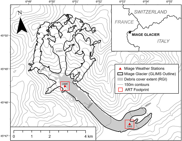
FIGURE 1. Site map of Miage Glacier showing weather station locations (LWS = lower weather station and UWS = upper weather station). The symbology of the weather stations reflects the grids shown in Figure 2. The insert shows the regional location of the study area. Contours produced using Copernicus data and information funded by the European Union—EU-DEM layers. https://www.eea.europa.eu/data-and-maps/data/copernicus-land-monitoring-service-eu-dem.
2.2 CO2 gas flux measurement
Direct measurement of the near-surface vertical CO2 flux in mg m−2 s−1, Fc, was made using an open-path eddy covariance system, referred to as the EC system hereafter, consisting of a CSAT3 three-dimensional sonic anemometer and an EC150 CO2/H2O open path infra-red gas analyser, supplied by Campbell Scientific Ltd., Loughborough, United Kingdom (Table 1). The principles of trace gas flux measurement over glaciers using EC systems have been explained elsewhere, e.g., Wang and Xu (2018), and so are not repeated here. The EC system was installed at two separate sites in two different years to examine Fc variation over differing debris thickness and elevation: i) a lower weather station (LWS) at 2,000 m a.s.l., with mean debris thickness of 0.23 m, typical of the relatively thick debris present over much of the lower glacier, in the 2013 ablation season; and ii) an upper weather station (UWS) at 2,380 m a.s.l, with mean debris thickness of 0.04 m, representative of thin debris on the upper part of the continuously debris covered zone, in the 2016 ablation season. Both sites were located at the centre of level areas of the glacier surface, with little elevation variation within ∼50 m of the LWS, and ∼10 m of the UWS, with an upglacier slope of ∼6° starting at a distance >10 m from the UWS (Figure 2). Surface debris around the measurement sites was mainly in the size range 0.10–0.40 m (long axis), with occasional boulders >1 m, at the LWS, and mainly <0.05 m (long axis) at the UWS. EC instruments were mounted surface parallel on cross arms at 1.83 m height, attached to a free-standing tripod, and oriented towards the dominant wind direction (westerly at the LWS and north-westerly at the UWS) to minimise airflow shadowing by the tripod and the mounting apparatus. The measurement height at a little below 2 m was considered a suitable distance from the surface to capture dominant turbulent eddies in the airflow, whilst not seriously violating the assumption of the constant flux layer. Previous work at the LWS site revealed an absence of katabatic flows, due to convection from the debris cover, with the wind speed maximum normally located above 2 m from the surface (Brock et al., 2010).
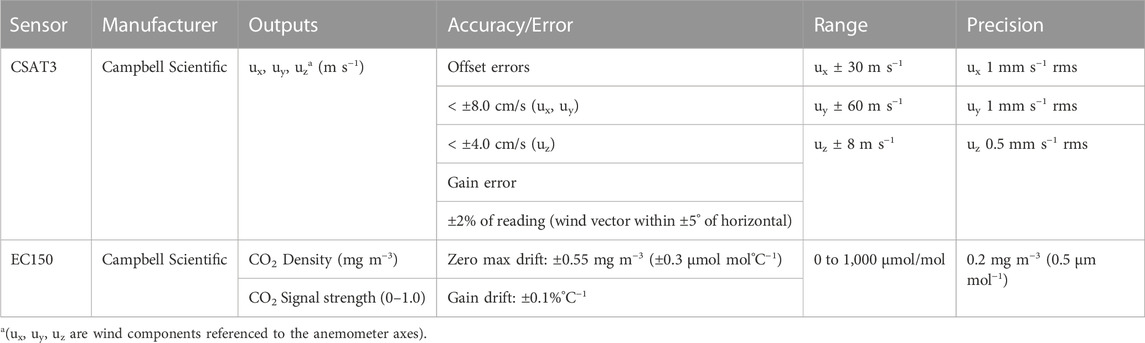
TABLE 1. Eddy covariance sensor specifications and accuracy.
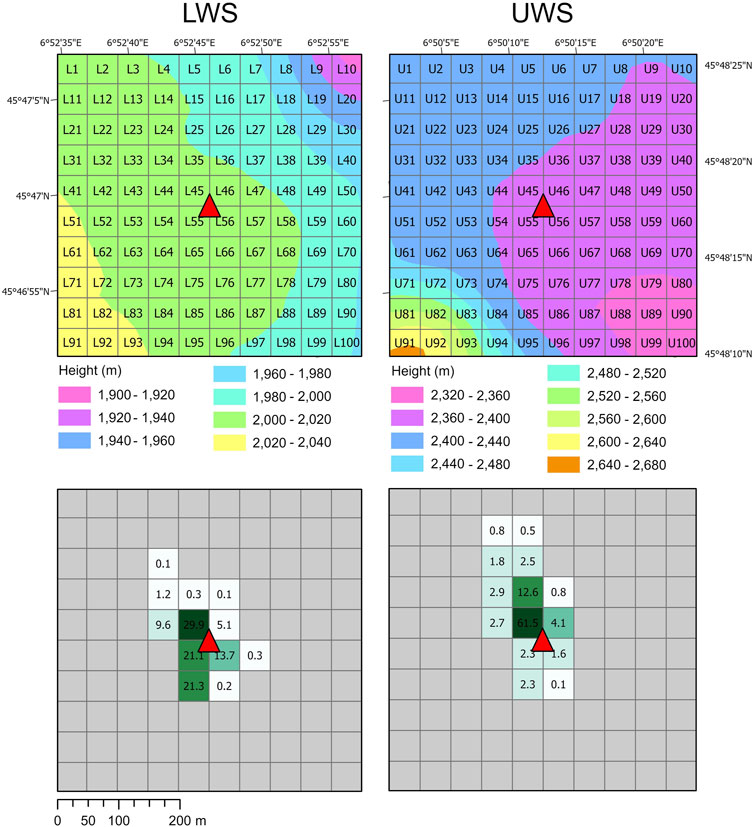
FIGURE 2. Spatial distribution of surface elevation (top row) and CO2 footprint contribution from ART model runs (bottom row) in 50 × 50 m cells around the LWS (left column) and UWS (right column). The location of the weather stations is denoted by the red triangle.
EC measurements were conducted between 26th June and 6th September 2013 at the LWS, and 24th June and 8th September 2016 at the UWS. 20 Hz measurements were recorded on a Campbell Scientific CR3000 datalogger and processed into 30-min averages using Campbell Scientific Open Path Eddy Covariance software (www.campbellsci.com). Corrections to the raw data were applied as follows: removal of unreliable values using sonic anemometer and gas analyser diagnostic codes; removal of low signal strength values (<90% full signal); lagging of CO2 measurements against sonic wind measurements using a covariance maximisation procedure; and application of the “WPL” flux correction for air density fluctuations (Webb et al., 1980). Outlying values in the 30-min averages, defined as Fc fluxes greater than +/- 3 standard deviations about the mean, were also removed prior to further analysis. The majority of removed data were due to: i) rain or condensation lying on the sensor nodes reducing signal strength; and ii) data gaps due to power or logger failures, in particular between 16 July and 10 August 2013. The number of remaining half hour values were 1,941 at the LWS and 2,928 at the UWS. Measurement sites were monitored every 1–2 days in late June, early July, and early September, and on 1 day in early August, and minor adjustments made to level instruments due to differential ablation beneath the tripod feet.
Under stable atmospheric conditions with low wind speed, turbulent mixing may be insufficient for CO2 absorbed or released at the surface to reach the instrument level. Estimation of the sub-instrument CO2 storage is an important consideration in ecological studies where instrument heights are typically several metres above the vegetation surface and biological activity and surface roughness are high. However, over supraglacial debris, unstable atmospheric conditions dominate during ablation periods and wind speeds are high and sustained, even during the night (Brock et al., 2010). Only 0.3% of the total half hour records had a friction velocity <0.05 m s−1, and no records had a friction velocity <0.01 m s−1, indicating that periods of weak turbulent mixing were rare. Wang and Xu (2018) identified the daily atmospheric CO2 storage in the debris area of Koxkar glacier to be less than 1% of net glacier carbon exchange, which they attributed to the low instrument height (2 m) limiting space for CO2 storage and the porous nature of the surface material. Due to the low likelihood of substantial surface CO2 storage, it was not considered in analysis of Fc in this study.
2.3 Measurement of independent meteorological variables
Both EC measurement sites were equipped with additional meteorological sensors to enable analysis of Fc variations using independent environmental variables. Air temperature, Ta (°C), and relative humidity (%) were measured using a HMP45C temperature and relative humidity sensor, housed inside a naturally ventilated Met21 radiation shield (both Campbell Scientific Ltd.). The Met21 radiation shield has been shown to be effective at protecting temperature sensors from anomalous solar heating on a debris-covered glacier (Shaw et al., 2016). The 4 components of the surface radiation balance (incident and reflected shortwave radiation, S↓ and S↑, respectively, and incoming and outgoing longwave radiation, L↓ and L↑, respectively; all in units of W m−2) were measured using Kipp and Zonen CNR1 (LWS) and CNR4 (UWS) radiometers. All instruments were mounted at 1.83 m, except the radiometers, which were mounted at 1.6 m. The instrument setup was very similar to that described in Brock et al. (2010) and full sensor specifications can be found in that paper. Hourly precipitation totals were obtained from the Lex Blanche weather station, operated by Regione Valle d’Aosta, 4 km west of the LWS at 2,162 m a.s.l. in both 2013 and 2016. Additional hourly precipitation data were available from a rain gauge at 2,340 m a.s.l. on Miage Glacier in 2013. The incoming and outgoing longwave radiation fluxes were used to calculate debris surface temperature, Ts, using a surface emissivity of 0.94, following Brock et al. (2010). Wind speed, u (m s−1), was calculated from the two horizontal wind speed components recorded by the sonic anemometer.
2.4 Surface conditions and modelling of contributing areas
To help understand processes controlling Fc recorded at the EC stations, the upwind contributing glacier surface areas, or footprints, were calculated. A particular consideration at the LWS site is the presence of forested areas 0.5–1.0 km distant which could influence Fc through photosynthesis and soil microbial processes. We calculated contributing areas using the Agroscope Reckenholz Tanikon (ART) footprint tool (Version 1.0, 13.03.2007) developed by the Swiss Federal Agricultural Research Center (Neftel et al., 2008). The ART footprint model is based on the analytical footprint model of Kormann and Meixner (2001) and has been successfully applied in the complex terrain of a debris-covered glacier (Wang and Xu, 2018).
Using analysis for all days of EC data, the glacier surface footprints at each site remain constant throughout the season and are dominated by areas <200 m from the EC stations (Figure 2). The main contributing areas are upglacier from the measurement sites corresponding with dominant wind direction (Figure 3); to the west of the LWS, with a small additional component from the south-east, and to the northwest of the UWS. The contribution of non-glacier areas was <0.1% at both sites, and hence off-glacier photosynthesis and respiration can be discounted as a significant influence on Fc recorded at the EC stations. No snow was recorded in the vicinity of the LWS during the 2013 measurement period. At the UWS, there was a continuous snow cover starting a few metres upglacier of the EC station in late June, coincident with the main contributing area. The snow cover had retreated several hundred metres upglacier by mid-July. Snow cover will therefore influence Fc at the UWS only in the first 2–3 weeks of the 2016 measurement period.
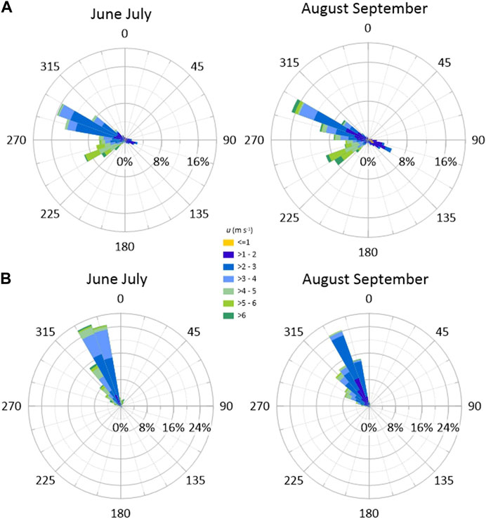
FIGURE 3. Half season wind roses for Miage Glacier at (A) LWS and (B) UWS. The radial scale shows the frequency of half hour mean winds blowing from a particular direction.
2.5 Data analysis
In the results section, Fc is presented visually for each site as daily and half-hourly time series, and as mean daily cycles using season-averaged values for each hour of the day. Regression analysis of half hourly Fc on independent meteorological variables (S↓, Ts, Ta, and u) is conducted on day (S↓ >0 W m−2), night (S↓ ≤0 W m−2) and half season (June-July = early season; August-September = late season) data subsets. The former subdivision is made due to the contrasting temperature regimes of debris in the day and night, and the latter subdivision is made to aid assessment of potentially influential long-term changes such as snow cover retreat, depletion of available reactive sediment within debris covers, and decline in S↓ between the early and late season. An alpha level of 0.05 is used to identify significant relationships. As is conventional in glaciological research, in this study fluxes of energy and mass are considered positive when directed towards the surface and negative when directed away from it.
3 Results
3.1 Seasonal trends in Fc and meteorological variables
At the LWS, daily net total Fc is positive for most days of the 2013 ablation season, with a mean of 1.58 g m−2 d−1, indicating a net downward flux of CO2 into the debris (Figure 4A, top trace). In the late June to mid-July period, daily total Fc varies between 1.5 and 3.0 g m−2 d−1, except for a value of 0.6 g m−2 d−1 on 9 July. Daily net total Fc remains positive on most days from mid-August to early September, but values are slightly lower, typically in the range 0.8–2.4 g m−2 d−1, with negative values on 19 and 24 August, and values close to zero on 23 and 27 August, and 4 September. Daily net total Fc does not exceed 2.0 g m−2 d−1 after 29 August.
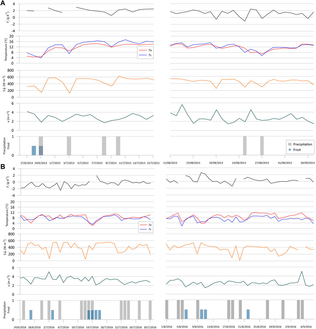
FIGURE 4. Half season daily averages of precipitation, u, S↓, Ta, Ts, and net daily total of Fc at the (A) LWS in 2013, and (B) UWS in 2016. Precipitation and ground frost are shown as binary series, with values of 1 and 0.5 indicating days with >0.4 mm of rain (grey bars) and ground frost (blue bars), respectively. Values on 29/06 and 03/07 in 2013 and values on 14/07, 05/08, 20/08, and 05/09 in 2016 are likely to have been skewed due to a large number of missing half hour values due to rainfall, hence Fc values are not shown for these dates. The data gap at the LWS (16/07 to 10/08) was due to logger failure. Positive Fc indicate downwardly directed fluxes, and negative Fc values indicate upwardly directed fluxes.
Fc values at the LWS broadly correspond with the pattern of daily average S↓, Ta, and Ts over the 2013 season, particularly in June and July (Figure 4A). Days with high positive Fc are generally concurrent with high S↓ and Ts, indicating warm and sunny weather conditions, while low positive or negative daily Fc totals, e.g., on 9 July, and 19, 24, and 27 August, correspond with marked drops in S↓ and Ts (Figure 4A), associated with relatively cool and cloudy conditions. There are some exceptions, e.g., daily Fc values decline between 4 and 7 July, while Ta and Ts increase, and S↓ remains steady, over the same period, and daily Fc totals appear to be independent of S↓, Ta, and Ts in the first week of September. There is no clear relationship between u and Fc at the LWS site, with days of high u corresponding with both high and low Fc. The days with the highest positive Fc totals in their respective half season periods: 30 June (2.8 g m−2 d−1) and 4 July (3.0 g m−2 d−1), and 25, 26, and 29 August (2.1–2.4 g m−2 d−1), are preceded by days of heavy rainfall (daily totals in the range 6–33 mm) and, in most cases, very low debris surface temperatures. Ts minima were <0°C on the mornings of 28 and 29 June, and <0.5°C on the mornings of 26 and 28 August. A data gap on 25 June means the minimum for that morning is not known. However, Ts remained well above 0°C throughout 4 July, and several days in August had Fc totals >2.0 g m−2 in the absence of rain or very low Ts.
At the UWS site, daily total Fc totals are predominantly negative, or close to zero, in the early season June to July period, with a mean of −0.5 g m−2 d−1, indicating a net upward flux of CO2 from debris to the atmosphere (Figure 4B, top trace). Daily Fc totals are most strongly negative in June and the first half of July, with values in the range −2.5 to +0.2 g m−2 d−1. In the second half of July, daily Fc totals are close to zero, ranging from −1.0 to +0.6 g m−2 d−1, except for a notable high positive total of 1.9 g m−2 d−1 on 15 July. In contrast to the June-July period, daily Fc totals are generally slightly positive in August and September, typically ranging from −0.6 to +1.7 g m−2 d−1, with a mean of +0.4 g m−2 d−1, indicating a net downward flux of CO2 to the debris in the second half of the 2016 season. There are large positive totals of 2.6 and 2.2 g m−2 d−1 on 10 and 11 August, respectively, and a large negative total of −1.4 g m−2 d−1 on 18 August. The mean daily total Fc at the UWS site over the 2016 season is −0.06 g m−2 d−1; one-16th of its magnitude of the LWS site in 2013, and of opposite sign.
There is no clear visual relationship between daily total Fc and daily mean S↓, Ta, Ts, and u at the UWS in the period from late June to the middle of August 2016 (Figure 4B). A weak direct relationship between daily total Fc and daily mean S↓, Ta and Ts is apparent in the second half of August and first week of September, however, but Fc still appears to be independent of u. In similarity to the LWS, the days with the highest positive daily Fc at the UWS, in the range 1.7–2.6 g m−2 d−1 on 15 July, and 6, 10, and 11 August 2016, all occurred on days with morning Ts <0°C, following heavy rain on the previous day (Figure 4B). Meteorological conditions were similar on these days, but not unusual in comparison to the rest of 2016, with relatively high S↓, and slightly below average Ta and Ts. Other days with morning Ts values <0°C: 27 June, 3 July, and 22 August, also show increased Fc totals compared with neighbouring days. Similarly, the 6 July, the only day in the first 3 weeks of the 2016 season with a positive Fc, total had low Ts (<0.5°C in the early morning) following heavy rain on the preceding day.
3.2 Mean daily cycle of Fc
At the LWS, hourly-averaged Fc displays a strong diurnal cycle with an approximately bell-shaped curve of positive daytime values, centred on an early afternoon peak, while the night-time Fc is characterised by negative values of smaller magnitude, with no clear relationship to the time of night (Figures 5A, 6A). On an average day in the 2013 season, the LWS Fc is positive for 12 h between 8.00 and 20.00, peaking at >90 mg m−2 s−1 (>0.3 g m−2 h−1) between 14.00 and 15.00, while night-time Fc drops to −14 mg m−2 s−1 (−0.05 g m−2 h−1) between 22.00 and 23.00, and then varies in a narrow range between −8 and −15 mg m−2 s−1 (approximately −0.03 to −0.05 g m−2 h−1) until 8.00. Peak half-hour Fc exceeds 140 mg m−2 s−1 (>0.5 g m−2 h−1) in several days in June, July, and August (Figure 5A). Both the magnitude and variability of night-time Fc increases from late June to the middle period from mid-July to mid-August, with peak half-hour Fc occasionally exceeding −50 mg m−2 s−1, (−0.18 g m−2 h−1) before reducing in magnitude again in late August and early September, although still with a high amount of variability (Figure 5A).
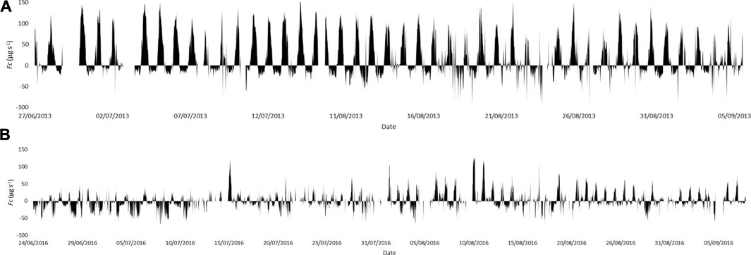
FIGURE 5. Time series of half hourly Fc at the: (A) LWS and (B) UWS throughout the monitoring period.
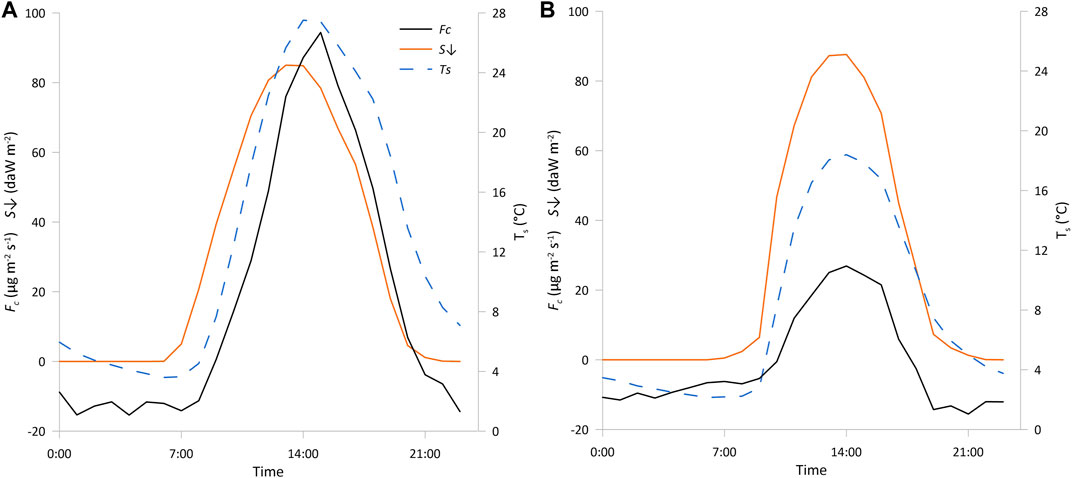
FIGURE 6. Daily average cycles of Fc, S↓, Ts at the (A) LWS and (B) UWS. Downwards directed Fc are represented by positive values and upwards directed Fc by negative values.
At the UWS site, hourly-averaged Fc shows a similar pattern of positive daytime, and negative night-time values, but with lower magnitude in the daytime, around one-third of that at the LWS, while night-time values are in a similar range at both sites (Figures 5B, 6B). The UWS site also shows greater temporal variability in both day and night Fc over the 2016 measurement period compared with the LWS site (Figure 5). At the UWS, Fc transitions from the early period up to the middle of July, which is dominated by relatively high negative night-time flux and weak positive daytime flux, through the second half of July when positive daytime and negative night-time fluxes are approximately in balance, to the August-September period when positive daytime fluxes generally exceed negative night-time fluxes. On an average day in the 2016 season, the UWS Fc is positive for 7 h between 10.00 and 17.00, peaking at 27 mg m−2 s−1 (∼0.1 g m−2 h−1) between 13.00 and 14.00, while night-time Fc drops to −16 mg m−2 s−1 (−0.06 g m−2 h−1) between 20.00 and 21.00, and then gradually increases over the remainder of the night, reaching −5 mg m−2 s−1 (−0.02 g m−2 h−1) between 8.00 and 9.00 (Figure 6B). Daytime, half-hour Fc rarely exceeds 60 mg m−2 s−1, (∼0.2 g m−2 h−1) but peak fluxes over 110 mg m−2 s−1 (∼0.4 g m−2 h−1) are recorded on 3 days, all of which had morning Ts <0°C (Figure 5B).
3.3 Relationship between mean daily cycles of Fc, Ts, and S↓
There is a striking similarity in the form and temporal alignment of the mean daytime cycles of Fc, Ts, and S↓ at both sites (Figures 6A, B). At the LWS site, the initial morning rise and daytime peak of S↓ occur 1 hour earlier than the corresponding inflection points in the Fc curve, whereas Ts and Fc vary in unison, with temporally aligned inflection points in the morning, early afternoon, and evening. At the UWS site, the initial morning rise in S↓ occurs 1 hour earlier than the corresponding rises in Fc and Ts, however, the peak values of all 3 variables occur together between 13.00 and 14.00, and their evening inflection points are similarly temporally aligned. While S↓ is of similar magnitude at the LWS and UWS in the 10.00–17.00 high flux period, with mean values of 747 and 743 W m−2, respectively, Fc and Ts values over the same period are much lower at the UWS, at 28% and 67% of their LWS values, respectively. The duration of high S↓ values over 100 W m−2 is 3 h shorter at the UWS compared with the LWS due to topographic shading in the early morning and evening. During the night, hourly mean Ts gradually decreases from the late evening to a minimum value between 5.00 and 6.00 at both sites, while over the same period Fc contrasts between a gradual and variable increasing trend at the UWS, and no trend with small variability at the LWS.
3.4 Statistical analysis of the relationship of Fc to meteorological variables
Results of the statistical analysis are presented in Tables 2, 3; Figures 7, 8.
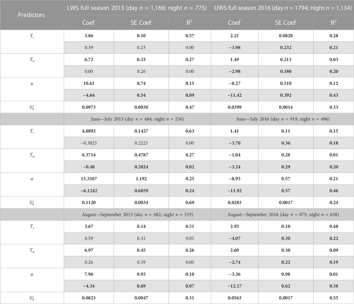
TABLE 2. Regression analysis of Fc (half hourly values) on meteorological variables. Fc in mg m−2 s−1; Ts and Ta in °C, u in m−2 s−1 and S↓ in W m−2. Shaded rows indicate night analyses and clear rows indicate day analyses. Significant relationships are denoted by bold values (p ≤ 0.05).
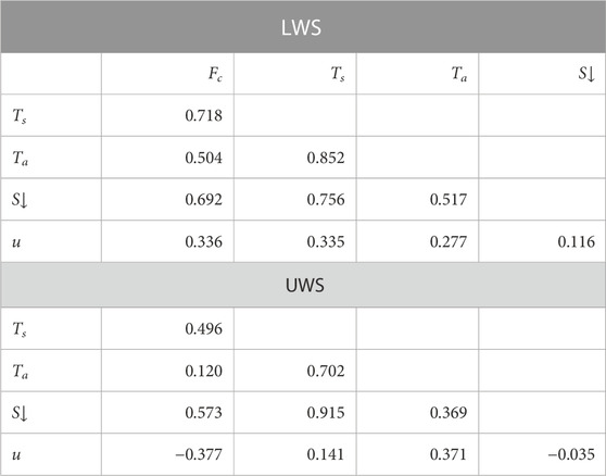
TABLE 3. Correlation matrix of Fc and environmental variables. All correlations are significant at p ≤ 0.05.
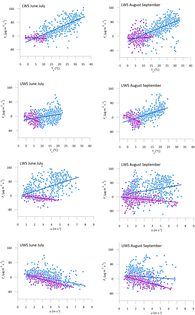
FIGURE 7. Relationships of Fc to surface temperature (Ts, top four plots) and wind speed (u, bottom four plots) at: the LWS (rows 1 and 3) and UWS (rows 2 and 4) in June-July (left column) and August-September (right column). Daytime and night-time half hourly mean values are shown by the blue and purple circles, respectively, together with best linear least squares regressions (blue and purple lines). Downwards directed Fc is represented by positive values and upwards directed Fc by negative values.
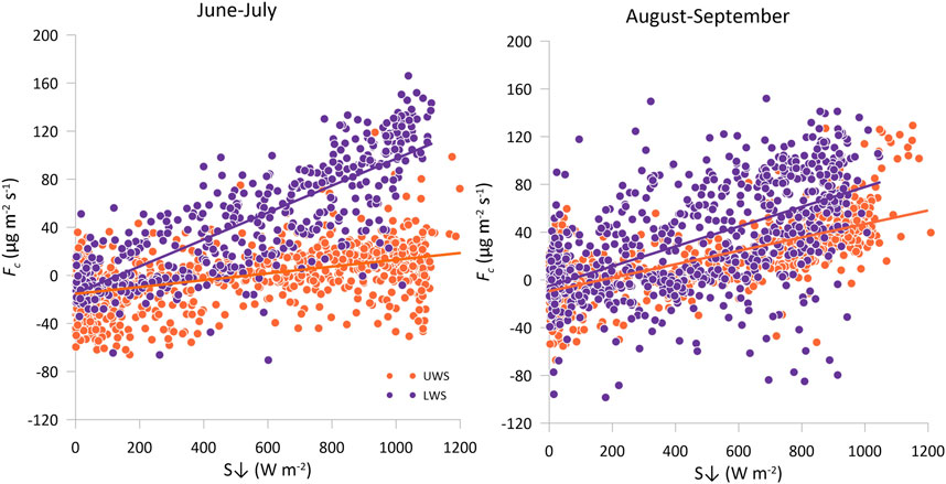
FIGURE 8. June-July and August-September relationship of Fc to incoming shortwave radiation (S↓). LWS and UWS values are shown by purple and orange circles, respectively, together with best fit linear least squares repressions (purple and orange lines). Downwards directed Fc is represented by positive values and upwards directed Fc by negative values.
Daytime Fc has significant direct relationships to Ts, and S↓ at both the LWS and UWS sites and in both half-season and full season data sets. The simple linear regression relationships are strongest at the LWS, particularly in the June-July period when Ts, and S↓ each account for >60% of the variance in daytime Fc, with the slight lag between daytime cycles of Fc and independent variables (Figure 6) and associated hysteresis accounting for some of the unexplained variance. The relationships of Fc to Ts, and S↓ at the UWS are weak, although significant, in the June-July period but become much stronger in August-September when S↓ explains a greater amount of Fc variance than at the LWS. The slope coefficients for the regressions of Fc on Ts, and S↓ at the LWS decrease between June-July and August-September indicating a lower sensitivity of Fc to debris surface temperature and incoming shortwave radiation in the second half of the season. In contrast, at the UWS the corresponding slope coefficients increase between June-July and August-September, approximately doubling the sensitivity of Fc to Ts, and S↓ in the second half of the season, although still with lower sensitivity than at the LWS. The scatter of high magnitude negative daytime Fc values, visible in the LWS graphs, particularly in August-September (Figure 7 top two panels and Figure 8), is mostly associated with rainfall events when it is possible that water interfered with gas analyser measurements, even though the instrument signal strength was above threshold. Hence, the decrease in slope coefficients and R2 values between June-July and August-September for the relationships of Fc to Ts, and S↓ at the LWS may be at least partly due measurement error, rather than purely due to change in physical process.
Daytime Fc has significant direct relationships to Ta and u at the LWS, with the slope coefficient and R2 value for the Ta relationships quite consistent between June-July and August-September but dropping markedly for the u relationships over the same period (Table 2). In contrast, daytime Fc has a weak, although significant, dependency on Ta at the UWS, changing from an inverse to a direct relationship between June-July and August-September. The relationship of daytime Fc to u at the UWS is significant and inverse in both periods, changing from a moderately strong relationship in June-July to a very weak relationship in August-September. The night-time relationships of Fc to Ts and Ta at the LWS are either weak or non-significant, but Fc has a moderately strong and significant inverse night-time relationship to u in June-July, becoming weak, although still significant, in August-September (Table 2; Figure 7). In contrast, at the UWS night-time Fc has moderately strong and significant inverse relationships to Ts, Ta, and u in both June-July and August-September. In particular, u accounts for almost half of night-time Fc variance at the UWS in June-July, and over a third in August-September.
A stepwise regression procedure was used to develop multivariable relationships to explain Fc variance, whilst accounting for collinearity between independent variables, with the resulting significant relationships for Fc in mg m−2 s−1 as follows:
LWS daytime:
UWS daytime:
LWS night-time:
UWS night-time:
All four meteorological variables (Ts, Ta, S↓ and u) independently explain part of the daytime Fc variance at the LWS, with Ts accounting for the largest portion, and S↓ and u the least, and these relationships have very high coefficients of determination, particularly in June-July (Eqs 1–3). Fc sensitivity to Ts and Ta increases between June-July and August-September but decreases for S↓ and u. Interestingly, the Ta slope coefficient reverses from a positive value in the simple linear regressions (Table 2) to a negative value in the multiple regression relationships (Eqs 1–3). This implies that the apparent positive relationship of Fc to Ta in the simple linear regressions is most likely spurious and due to the strong positive correlation of Ta with Ts and S↓ (Table 3). The UWS June-July daytime multiple regression relationship (Eq. 5) has a lower R2 and a different form to the LWS daytime relationships (Eqs 1–3), with Fc most strongly dependent on S↓, independent of Ts, weakly dependent on Ta, and with an inverse relationship to u. In contrast, the UWS August-September daytime multiple regression relationship and coefficient of determination (Eq. 6) are similar to the August-September daytime LWS relationship (Eq. 3), except that Fc at the UWS is independent of S↓.
The LWS night-time multiple regression relationships account for only a small proportion of Fc variance, almost entirely associated with the inverse relationship of Fc flux to u, despite the inclusion of Ts and Ta as independent variables (Eqs 7–9). By comparison, the UWS night-time relationships have higher coefficients of determination, particularly in June-July, which again is almost entirely dependent on the inverse relationship of Fc flux to u, with Ta accounting for only a small part of Fc variance (Eqs 10–12).
4 Discussion
4.1 Fc magnitude on debris covered glaciers
The seasonal Fc values infer that thick supraglacial debris is a net CO2 sink over the ablation period, while on thin supraglacial debris net CO2 exchange is close to zero. Assuming the LWC EC measurements are representative for thick debris generally, the mean downward flux of 1.58 g m−2 d−1 would equate to 1.58 t CO2 km−2 d−1. With thick debris extending well over 3 km2 over the glacier’s surface (Mihalcea et al., 2008; Foster et al., 2012) total drawdown over a 100-day ablation season (a conservative estimate for Miage glacier; Brock et al., 2010) could be of the order of 500 t CO2 (0.5 Gg CO2). In units of carbon, the total ablation season drawdown for the thick debris area at Miage Glacier would be ∼43 t C km−2. For comparison, this is 4 times the very high drawdown rate estimated for marginal surface areas of the Greenland Ice Sheet associated with CO2 consumption by photoautotrophic algae (Cook et al., 2012).
EC measurements of Fc over supraglacial debris are rare. To our knowledge, the only other comparable study is that of Wang and Xu (2018), who reported a net downwardly oriented Fc of 58.68 mmol m−2 d−1 (equivalent to 2.58 g m−2 d−1) over 2 years of EC measurements at Koxkar Glacier, western Tien Shan. The Koxkar Glacier site was at higher elevation (3,212 m) and on thicker debris (0.72 m) than the Miage glacier sites and included measurements during the winter accumulation and spring snow melt periods, as well as the summer ablation season. However, the magnitude of Fc is similar at both glaciers, and this strongly suggests that debris-covered glaciers with extensive covers of thick cover of silicate rocks are important to local and regional carbon cycling. Without data from outside of the ablation season, the net annual Fc at Miage glacier cannot be determined, although the small number of measurements at Ts<0°C suggest Fc magnitude becomes very small at negative temperatures. Wang and Xu (2018) observed that low rates of CO2 drawdown continued in winter at Koxkar Glacier, even when debris was snow covered and melting absent.
4.2 Processes controlling Fc magnitude and direction
The high magnitude daytime downward Fc at the LWS site, and at the UWS site in the mid July to early September period, is most likely due to CO2 drawdown induced by a combination of hydrolysis and carbonation reactions. During the day, the debris is warmed by solar radiation, and heat energy is conducted downwards through the debris layer leading to melting of ice at the debris interface (Reid and Brock, 2010). The rates of both diffusion of atmospheric CO2 into meltwater and rock chemical weathering will increase when Ts increases, because: i) the supply of fresh low p(CO2) meltwater is greatest when debris surface temperature is highest; and ii) the rate of chemical reaction increases with temperature (Arrhenius principle). These interlinked processes generate a daytime Fc cycle which corresponds closely with, but slightly lags, the daytime cycles of S↓ and Ts (Figure 6). Fyffe et al. (2019b) established that surface meltwater at Miage Glacier flows through debris and drains into supraglacial streams, and so water in the debris matrix could be replenished by new ice melt before it becomes saturated in dissolved CO2. The combination of the melt-driven supply of fresh dilute water, high temperatures, and reactive mineral surfaces open to the atmosphere makes supraglacial debris an ideal environment for rock chemical weathering and consumption of atmospheric CO2 during the ablation season. With these conditions, daytime CO2 drawdown rates can exceed 0.5 g m−2 h−1 when Ts exceeds 30°C, but approach zero when Ts ≤0°C (Figure 7). S↓ and daytime Ts both correlate strongly with Fc (Table 2) but this consideration of processes, and the lag between increasing S↓ and Fc in the morning (Figure 6), points to a primary role for insolation in providing energy to heat debris and drive melting, rather than being a direct control on Fc. Similarly, daytime Ta and u correlate with Fc primary because their daily cycles are controlled to a great extent by Ts (Brock et al., 2010).
The strong relationship of Fc to Ts and S↓ is consistent between the early and late season at the LWS, and late season at the UWS (Table 2; Eqs 2, 3, 6; Figures 7, 8). The early season period at the UWS is distinct, however, with Fc only weakly dependent on S↓ and Ts (Table 2; Eq. 5; Figures 7, 8), and of much lower daytime magnitude, particularly in the first 3 weeks, than in the remainder of the 2016 season (Figure 4B, upper trace). This cannot be explained by changing meteorological conditions because Ts, Ta, S↓, and u are very similar between the early and late ablation season (Table 4). The most likely explanation is the presence of extensive snow cover in the area upwind from the UWS in the early part of the 2016 ablation season. Trace gases can diffuse through seasonal snow cover (e.g., Seok et al., 2009) so the likely control of snow cover on Fc is the inhibition of processes of CO2 uptake in debris. The high albedo and low thermal conductivity of snow will strongly reduce the heat flux to the underlying debris, suppressing ice melt and rock weathering, and limiting the consumption of atmospheric CO2 through carbonation. The UWS site itself was already snow free when the EC station was installed, enabling the debris there to warm in response to daytime insolation. Hence, there would have been a mismatch between the sample area of S↓ and Ts, unaffected by snow cover at, or close to, the UWS site, and the snow-covered CO2 footprint area extending 200 m upglacier, resulting in weak relationships of Fc to S↓ and Ts. Over time, the snow cover retreated, gradually increasing the area of exposed debris in the UWS contributing area. The 4-day rain event from 11 to 14 July 2016 (Figure 4B) likely removed most of the remaining snow cover within 200 m of the UWS, and subsequently daytime Fc magnitude increased (Figure 5B) and daily Fc totals transitioned from strongly negative to close to zero (Figure 4B).

TABLE 4. Seasonal averages of environmental variables.
Two pieces of evidence imply that the rate of daytime CO2 drawdown is sediment limited. First, the sensitivity of daytime Fc to Ts is lower at the thin debris UWS site compared to the thick debris LWS site (Table 2; Figure 7) and Fc is greater at the LWS than the UWS for the same debris surface temperatures at all values of Ts> 8°C. Meltwater supply rate cannot be the reason for lower daytime Fc at the UWS since ice melt rates would generally be higher at the UWS due to the lower thermal resistance of thin debris cover (Reid and Brock, 2010; Fyffe et al., 2014). The likely explanation for lower Fc at the UWS is the smaller debris-water contact area in the 0.04 m debris layer, compared with the 0.23 m layer at the LWS, resulting in a lower rate of hydrolysis and atmospheric CO2 drawdown.
Second, daily total Fc is higher on days following rain-debris frost events. At the UWS, daily Fc totals on 15 July and 6, 7, 10, and 11 August 2016 are >1.5 g m−2 d−1, much higher than the mean daily UWS flux of −0.06 g m−2 d−1 and comparable to the mean daily Fc total at the LWS of 1.58 g m−2 d−1 (Figure 4). Similarly, the second highest daily Fc total at the LWS occurred on 30 June following a rain-debris frost event (Figure 4). These results implicate the role of frost shattering in supplying comminuted reactive sediment for chemical reactions in the debris layer, particularly in thin debris covers. Freshly exposed mineral surfaces are highly reactive in contact with water (St Pierre et al., 2019; Wadham et al., 2019) and would be rapidly chemically weathered with the onset of debris warming and ice melt in the day following the frost, in turn leading to a transitory acceleration in atmospheric CO2 drawdown. Saturation of rocks by rain followed by sub-zero temperatures, as occurred in the debris frost events identified (Figure 4), creates ideal conditions for mechanical fracture of rock clasts, due to the stress applied by expansion of freezing water in pores and along grain boundaries (Matsuoka, 1990). During fieldwork, recently shattered clasts were frequently observed on and in the debris cover, particularly in the higher parts of the debris-covered zone. There were some days at the LWS site when daily total Fc exceeded 2 g m−2 d−1 without preceding rain or frost, suggesting the availability of recently shattered sediment is less of a control on CO2 drawdown rate in areas of thick debris. It is possible, however, that alluviation of shattered sediment by rain at the LWS on the 3 July 2013 supplied fresh reactive material to the lower water-saturated horizon of the debris layer, leading to the highest daily Fc total on 4 July. At the UWS, increases in Fc following debris frosts on 27 June and 3 July 2016 were of likely of small magnitude due to widespread snow cover at the time.
Night Fc is predominantly negative with similar magnitude at both sites: LWS night mean = −41 mg m−2 h−1 and UWS night mean = −35 mg m−2 h−1. The flux of CO2 to the atmosphere in the night is most likely due to respiration by debris-dwelling microorganisms dominating net surface CO2 exchange while hydrolysis and carbonation rates are low. Microbially-mediated sulphide oxidation, if present, could generate high p (CO2) in immobile pore waters located above the night-time water table, potentially adding to night-time CO2 emission. It is also possible that expulsion of dissolved CO2 during overnight freezing of water in the debris periodically contributes to the negative night-time Fc. In the daytime at low Ts, Fc is also negative and of similar magnitude to the night-time, for example, for Ts<6°C, daytime mean Fc is −32 mg m−2 h−1 at the LWS and −27 mg m−2 h−1 at the UWS. Hence, microbial respiration is not restricted to night-time, but its impact on net Fc in the daytime is normally masked by the much higher magnitude of CO2 consumption by hydrochemical reactions.
A noticeable difference between the two sites is that night-time Fc at the LWS is independent of Ts and Ta, and only weakly dependent on u, whereas at the UWS night-time Fc is significantly inversely dependent on all three independent variables (Table 2; Figure 7). The apparent relationship of night-time Fc to u, Ts and Ta at the UWS is likely to be spurious, however, because all four variables depend strongly on time of the night, with seasonally averaged hourly values decreasing almost monotonically from 8 p.m. to 8 a.m. For example, hourly averaged Fc and u correlate more strongly with hour since 7 p.m. (Pearson’s r values = 0.955 and 0.944, respectively) than they do with each other (Pearson’s r = 0.882). An alternative explanation for the night-time trend of decreasing Fc at the UWS lies in the differing water retention between thick and thin debris layers. Daytime meltwater would be expected to drain quickly from the thin debris layer at the UWS but be partly retained within thick debris at the LWS (Fyffe et al., 2019b). Heterotrophic activity in soils is known to be moisture limited (Manzoni et al., 2012). Hence, the decreasing magnitude of Fc over the course of the night at the UWS might be due to decreasing water availability limiting microbial activity, while water availability is not a restrictive factor at the LWS (Figure 6). In this context, the diurnal cycle of Fc (Figure 6) can be at least partly explained through the dynamics of the debris water table, with daytime flooding and night-time drainage of meltwater varying the mixing ratio of mobile low p(CO2) meltwater to immobile high p(CO2) porewater dominated by microbial respiration. Differences in respiration rate between the UWS and LWS might also relate to spatial variation in microbial communities on DCGs, which have been observed to increase in complexity and become increasingly heterotrophic downglacier, with increasing debris thickness and age (Franzetti et al., 2013; Darcy et al., 2017). At the UWS site, net release of CO2 during the early season (Figure 5B) suggests microbial respiration may be important during the late winter and early ablation period of snow cover retreat.
5 Conclusion
We have presented an analysis of near-surface atmospheric CO2 flux and its relationship to meteorological and environmental variables at contrasting thick and thin debris sites on an alpine debris-covered glacier over two ablation seasons, using eddy covariance measurements. The main conclusions are.
1. Miage glacier is a net sink of CO2 over the ablation season. The mean drawdown rate over a thick 0.23 m debris layer, typical of most of the debris-covered zone, was 1.58 g m−2 d−1 which, if spatially representative, implies a drawdown rate of >150 t CO2 km−2 over an ablation season, and over 500 t CO2 (0.5 Gg CO2), for the whole Miage glacier debris-covered zone. This rate is substantially higher than rates of CO2 uptake by photosynthesising microorganisms on the surface of the Greenland Ice Sheet (Cook et al., 2012) but similar to the rate measured on a thick debris layer at Koxkar Glacier, Tianshan Mountains, China (Wang and Xu, 2018).
2. The ablation season mean CO2 flux over a higher-elevation thin debris site, with mean thickness 0.04 m, was close to net zero, with a net rate of CO2 release to the atmosphere of 0.06 g m2 d1. This included an early period of snow cover, dominated by an upward flux of CO2 (mean flux = −0.5 g m2 d1). The net flux reversed sign following melting of the snow and the August-September period was dominated by net drawdown of CO2, albeit at a lower rate (mean flux = 0.4 g m2 d1) than at the lower thick debris site.
3. The high rate of drawdown is likely due to dissolution of CO2 in carbonation and hydrolysis reactions in wet debris layers. The combination of the melt-driven supply of fresh low p(CO2) water, high temperatures, and reactive mineral surfaces open to the atmosphere makes supraglacial debris an ideal environment for rock chemical weathering and consumption of atmospheric CO2 during the ablation season.
4. Mean CO2 flux alternates between downward and upward orientation in the day and night, respectively, and the night-time flux is around one-third of the daytime flux magnitude. The daytime flux has a pronounced curve, with the drawdown rate closely correlated with the cycle of debris surface temperature, peaking in the early afternoon. Solar radiation is an important driver in heating the debris layer, providing heat energy for ice melt and chemical weathering reactions; and CO2 flux is low on overcast days.
5. Net CO2 release to the atmosphere in the night, and in the daytime when debris surface temperature is below 7°C, is most likely due to respiration by microorganisms. Biological respiration almost certainly continues during the day, but only dominates the net CO2 flux at low temperatures when chemical weathering rates are low. Decreasing meltwater availability with time overnight may be a limiting factor on microbial activity in thin debris.
6. CO2 drawdown rates are controlled by the supply of fresh mineral surfaces and water, particularly on thin debris. On days following rainfall-debris frost events, daytime CO2 drawdown increased by an order of magnitude to a rate comparable to thick debris. Frost shattering of saturated debris during overnight freezing likely provides abundant fresh reactive sediment which is rapidly chemically weathered with the onset of ice melting the following day. An increase in daytime CO2 drawdown rate of lower magnitude was also observed following a debris frost event at the thick debris site.
Our results imply that debris-covered glaciers are important to local and regional carbon cycling, and further measurement of CO2 fluxes over supraglacial debris, and research into driving processes is warranted, considering the large and growing global extent of global supraglacial debris (Scherler et al., 2018; Herreid and Pellicciotti, 2020; Tielidze et al., 2020). Future studies should encompass different geological and climatic regions and involve geochemical analyses of rocks and meltwater to establish key hydrolysis reactions and the long-term fate of carbon exported as glacier runoff. Monitoring of temperature, pH, conductivity and p(CO2) of water in the debris layer, in conjunction with isotopic analyses to identify the source of carbon in runoff, could prove to be particularly insightful. Very few studies have investigated the microecology of debris covered glaciers, and more research, including DNA sequencing of debris rock/soil samples and taxonomic ecology, is needed to identify species and their functional roles in carbon cycling. Eddy covariance is found to be a suitable tool for monitoring the near-surface CO2 flux at short- and long-term timescales, but uncertainties in eddy covariance flux measurements and their interpretation at glacier sites (e.g., Nicholson and Stiperski, 2020) and its restriction to a small number of measurements sites, could be addressed though distributed sampling of CO2 fluxes, e.g., using portable gas analysers. These studies should lead to the development of a model for CO2 exchange in supraglacial debris that could be used to test understanding of key processes and provide estimates of fluxes at regional and global scales.
Data availability statement
The raw data supporting the conclusion of this article will be made available by the authors, without undue reservation.
Author contributions
BB conceived the study and led the data collection. GB led the data analysis and prepared the figures. All authors contributed to the article and approved the submitted version.
Funding
GB is supported by a UK Natural Environment Research Council (NERC) studentship (NE/S007512/1). Article processing charges were paid by the Northumbria University UKRI block grant.
Acknowledgments
We gratefully acknowledge provision of scientific equipment and support for fieldwork costs by Northumbria University. We give our thanks to Catriona Fyffe (Institute of Science and Technology, Austria), Mike Lim (Northumbria University, United Kingdom), Thomas Shaw (Swiss Federal Institute, WSL, Switzerland), Matt Westoby (University of Plymouth, United Kingdom) for help with glacier fieldwork, and Jean-Pierre Fosson, Marco Vagliasindi (Fondazione Montagna Sicura, Courmayeur, Italy), Edoardo Cremonese, Fabrizio Diotri (Agenzia Regionale per la Protezione dell’Ambiente Valle d’Aosta, Italy), and Philip Deline (Universite Savoie Mont Blanc, France) for fieldwork logistical support. We also thank two reviewers and Editor Xin Wang for their constructive comments on the manuscript.
Conflict of interest
The authors declare that the research was conducted in the absence of any commercial or financial relationships that could be construed as a potential conflict of interest.
Publisher’s note
All claims expressed in this article are solely those of the authors and do not necessarily represent those of their affiliated organizations, or those of the publisher, the editors and the reviewers. Any product that may be evaluated in this article, or claim that may be made by its manufacturer, is not guaranteed or endorsed by the publisher.
References
Anesio, A. M., Hodson, A. J., Fritz, A., Psenner, R., and Sattler, B. (2009). High microbial activity on glaciers: Importance to the global carbon cycle. Glob. Change Biol. 15 (4), 955–960. doi:10.1111/j.1365-2486.2008.01758.x
Anesio, A., Sattler, B., Foreman, C., Telling, J., Hodson, A., Tranter, M., et al. (2010). Carbon fluxes through bacterial communities on glacier surfaces. Ann. Glaciol. 51 (56), 32–40. doi:10.3189/172756411795932092
Azzoni, R. S., Franzetti, A., Fontaneto, D., Zullini, A., and Ambrosini, R. (2015). Nematodes and rotifers on two Alpine debris-covered glaciers. Ital. J. Zool. 82 (4), 616–623. doi:10.1080/11250003.2015.1080312
Baldocchi, D. D. (2019). How eddy covariance flux measurements have contributed to our understanding of Global Change Biology. Glob. Change Biol. 26, 242–260. doi:10.1111/gcb.14807
Benn, D. I., Bolch, T., Hands, K., Gulley, K., Luckman, A., Nicholson, L. I., et al. (2012). Response of debris-covered glaciers in the Mount Everest region to recent warming, and implications for outburst flood hazards. Earth-Sci. Rev. 114, 156–174. doi:10.1016/j.earscirev.2012.03.008
Benn, D. I., Thompson, S., Gulley, J., Mertes, J., Luckman, A., and Nicholson, L. (2017). Structure and evolution of the drainage system of a Himalayan debris-covered glacier, and its relationship with patterns of mass loss. Cryosphere 11 (5), 2247–2264. doi:10.5194/tc-11-2247-2017
Brock, B. W., Mihalcea, C., Kirkbride, M. P., Diolaiuti, G., Cutler, M. E., and Smiraglia, C. (2010). Meteorology and surface energy fluxes in the 2005–2007 ablation seasons at the Miage debris-covered glacier, Mont Blanc Massif, Italian Alps. J. Geophys. Res. Atmos. 115 (D9), D09106. doi:10.1029/2009JD013224
Brown, G. H. (2002). Glacier meltwater hydrochemistry. App. Geochem. 17 (7), 855–883. doi:10.1016/S0883-2927(01)00123-8
Caccianiga, M., Andreis, C., Diolaiuiti, G., D’Agata, C., Mihalcea, C., and Smiraglia, C. (2011). Alpine debris-covered glaciers as a habitat for plant life. Holocene 21 (6), 2011–1020. doi:10.1177/0950683611400219
Collier, E., Nicholson, L. K., Brock, B. W., Maussion, F., Essery, R., and Bush, A. B. G. (2014). Representing moisture fluxes and phase changes in glacier debris cover using a reservoir approach. Cryosphere 8, 1429–1444. doi:10.5194/tc-8-1429-2014
Cook, J. M., Hodson, A. J., Anesio, A. M., Hanna, E., Yallop, M., Stibal, M., et al. (2012). An improved estimate of microbially mediated carbon fluxes from the Greenland ice sheet. J. Glaciol. 58 (212), 1098–1108. doi:10.3189/2012JoG12J001
Darcy, J. L., King, A. J., Gendron, E. M. S., and Schmidt, S. K. (2017). Spatial autocorrelation of microbial communities atop a debris-covered glacier is evidence of a supraglacial chronosequence. FEMS Microbiol. Ecol. 93 (8). doi:10.1093/femsec/fix095
Darcy, J. L., and Schmidt, S. K. (2016). Nutrient limitation of microbial phototrophs on a debris-covered glacier. Soil Biol. biochem. 95, 156–163. doi:10.1016/j.soilbio.2015.12.019
Deline, P. (2002). “Etude géomorphologique des interactions entre écroulements rocheux et glaciers dans la haute montagne alpine: Le versant sud-est du massif du Mont blanc (vallée d'Aoste, italie),”. Ph.D. thesis (Chambéry: Université de Savoie), 365.
Deline, P., Gardent, M., Magnin, F., and Ravanel, L. (2012). The morphodynamics of the mont blanc massif in a changing cryosphere: A comprehensive review. Geog. Ann. Ser. A 94 (2), 265–283. doi:10.1111/j.1468-0459.2012.00467.x
Deline, P. (2009). Interactions between rock avalanches and glaciers in the Mont Blanc massif during the late Holocene. Quat. Sci. Rev. 28, 1070–1083. doi:10.1016/j.quascirev.2008.09.025
Fairchild, I. J., Bradby, L., Sharp, M., and Tison, J.-L. (1994). Hydrochemistry of carbonate terrains in alpine glacial settings. Earth Surf. Process.Landf. 19, 33–54. doi:10.1002/esp.3290190104
Foster, L. A., Brock, B. W., Cutler, M. E. J., and Diotri, F. (2012). A physically based method for estimating supraglacial debris thickness from thermal band remote-sensing data. J. Glaciol. 58 (210), 677–691. doi:10.3189/2012JoG11J194
Franzetti, A., Tatangelo, V., Gandolfi, I., Bertolini, V., Bestetti, G., Diolaiuit, G., et al. (2013). Bacterial community structure on two alpine debris-covered glaciers and biogeography of Polaromonas phylotypes. ISME J. 7, 1483–1492. doi:10.1038/ismej.2013.48
Fyffe, C. L., Brock, B. W., Kirkbride, M. P., Black, A. R., Smiraglia, C., and Diolaiuti, G. (2019a). The impact of supraglacial debris on proglacial runoff and water chemistry. J. Hydrol. 576, 41–57. doi:10.1016/j.jhydrol.2019.06.023
Fyffe, C. L., Brock, B. W., Kirkbride, M. P., Mair, D. W. F., Arnold, N. S., Smiraglia, C., et al. (2019b). Do debris-covered glaciers demonstrate distinctive hydrological behaviour compared to clean glaciers? J. Hydrol. 570, 584–597. doi:10.1016/j.jhydrol.2018.12.069
Fyffe, C. L., Reid, T. D., Brock, B. W., Kirkbride, M. P., Diolaiuti, G., Smiraglia, C., et al. (2014). A distributed energy-balance melt model of an alpine debris-covered glacier. J. Glaciol. 60 (221), 587–602. doi:10.3189/2014JoG13J148
Fyffe, C. L., Woodget, A. S., Kirkbride, M. P., Deline, P., Westoby, M. J., and Brock, B. W. (2020). Processes at the margins of supraglacial debris cover: Quantifying dirty ice ablation and debris redistribution. Earth Surf. Process. Landforms 45, 2272–2290. doi:10.1002/esp.4879
Gobbi, M., Isaia, M., and De Bernardi, F. (2011). Arthropod colonisation of a debris-covered glacier. Holocene 21 (2), 343–349. doi:10.1177/0959683610374885
Graly, J. A., Drever, J. I., and Humphrey, N. F. (2017). Calculating the balance between atmospheric CO2 drawdown and organic carbon oxidation in subglacial hydrochemical systems. Glob. Biogeochem. Cycles 31 (4), 709–727. doi:10.1002/2016GB005425
Gulley, J., and Benn, D. I. (2007). Structural control of englacial drainage systems in Himalayan debris-covered glaciers. J. Glaciol. 53 (182), 399–412. Cambridge University Press. doi:10.3189/002214307783258378
Herreid, S., and Pellicciotti, F. (2020). The state of rock debris covering Earth’s glaciers. Nat. Geosci. 13 (9), 621–627. doi:10.1038/s41561-020-0615-0
Hiller, R., Zeeman, M. J., and Eugster, W. (2008). Eddy-covariance flux measurements in the complex terrain of an Alpine valley in Switzerland. Boundary-Layer Meteorol. 127 (3), 449–467. doi:10.1007/s10546-008-9267-0
Hodson, A., Anesio, A. M., Ng, F., Watson, R., Quirk, J., Irvine-Fynn, T., et al. (2007). A glacier respires: Quantifying the distribution and respiration CO2 flux of cryoconite across an entire Arctic supraglacial ecosystem. J. Geophys. Res. 112, G04S36. doi:10.1029/2007JG000452
Hodson, A., Anesio, A. M., Tranter, M., Fountain, A., Osborn, M., Priscu, J., et al. (2008). Glacial ecosystems. Ecol. Monogr. 78 (1), 41–67. doi:10.1890/07-0187.1
Hodson, A. J., Tranter, M., and Vatne, G. (2000), Contemporary rates of chemical denudation and atmospheric CO2 sequestration in glacier basins: An Arctic perspective, Earth Surf. Proc. Land 25, 1447–1471. doi:10.1002/1096-9837(200012)25:13<1447:AID-ESP156>3.0.CO;2-9
Kirkbride, M. P. (2011). “Debris-covered glaciers,” in Encyclopedia of snow, Ice and glaciers. Encyclopedia of Earth Sciences series. Editors V. P. Singh, P. Singh, and U. K. Haritashya (Dordrecht: Springer). doi:10.1007/978-90-481-2642-2
Kormann, R., and Meixner, F. X. (2001). An analytical footprint model for non-neutral stratification. Bound.-Layer Meteor 99, 207–224. doi:10.1023/A:1018991015119
Manzoni, S., Scimel, J. P., and Porporato, A. (2012). Responses of soil microbial communities to water stress: Results from a meta-analysis. Ecology 93, 930–938. doi:10.1890/11-0026.1
Matsuoka, N. (1990). Mechanisms of rock breakdown by frost action: An experimental approach. Cold Regions Sci. Technol. 17 (3), 253–270. doi:10.1016/S0165-232X(05)80005-9
Mihalcea, C., Brock, B. W., Diolaiuiti, G., D’Agata, C., Citterio, M., Kirkbride, M. P., et al. (2008). Using ASTER satellite and ground-based surface temperature measurements to derive supraglacial debris cover and thickness patterns on Miage Glacier (Mont Blanc Massif, Italy). Cold Reg. Sci. Tecnol. 52, 341–354. doi:10.1016/jcoldregions.2007.03.004
Miles, K. E., Hubbard, B., Irvine-Fynn, T. D. L., Miles, E. S., Quincey, D. J., and Rowan, A. V. (2020). Hydrology of debris-covered glaciers in High Mountain Asia. Earth-Science Rev. 207, 103212. doi:10.1016/j.earscirev.2020.103212
Neftel, A., Spirig, C., and Ammann, C. (2008). Application and test of a simple tool for operational footprint evaluations. Environ. Pollut. 152 (3), 644–652. doi:10.1016/j.envpol.2007.06.062
Nicholson, L., and Stiperski, I. (2020). Comparison of turbulent structures and energy fluxes over exposed and debris-covered glacier ice. J. Glaciol., 1–13. doi:10.1017/jog.2020.23
Nicholson, L., Wirbel, A., Mayer, C., and Lambrecht, A. (2021). The challenge of non-stationary feedbacks in modeling the response of debris-covered glaciers to climate forcing. Front. Earth Sci. 9, 662695. doi:10.3389/feart.2021.662695
Racoviteanu, A. E., Nicholson, L., Glasser, N. F., Miles, E., Harrison, S., and Reynolds, J. M. (2022). debris-covered glacier systems and associated glacial lake outburst flood hazards: Challenges and prospects. J. Geol. Soc. 179 (3), jgs2021–084. doi:10.1144/jgs2021-084
Raiswell, R. (1984). Chemical models of solute acquisition in glacial meltwaters. J. Glaciol. 30 (104), 49–57. doi:10.3189/S0022143000008480
Reid, T. D., and Brock, B. W. (2010). An energy-balance model for debris-covered glaciers including heat-conduction through the debris layer. J. Glaciol. 56, 903–916. doi:10.3189/002214310794457218
Rounce, D. R., Hock, R., McNabb, R. W., Millan, R., Sommer, C., Braun, M. H., et al. (2021). Distributed global debris thickness estimates reveal debris significantly impacts glacier mass balance. Geophys. Res. Lett. 48, e2020GL091311. doi:10.1029/2020GL091311
Rowan, A. V., Egholm, D. L., Quincey, D. J., and Glasser, N. F. (2015). Modelling the feedbacks between mass balance, ice flow and debris transport to predict the response to climate change of debris-covered glaciers in the himalaya. Earth Planet. Sci. Lett. 430, 427–438. doi:10.1016/j.epsl.2015.09.004
Scherler, D., Bookhagen, B., and Strecker, M. R. (2011). Spatially variable response of himalayan glaciers to climate change affected by debris cover. Nat. Geosci. 4, 156–159. doi:10.1038/ngeo1068
Scherler, D., Wulf, H., and Gorelick, N. (2018). Global assessment of supraglacial debris-cover extents. Geophys. Res. Lett. 45 (21), 11,798–11,805. doi:10.1029/2018GL080158
Seok, B., Helmig, D., Williams, M. W., Liptzin, D., Chowanski, K., and Hueber, J. (2009). An automated system for continuous measurements of trace gas fluxes through snow: An evaluation of the gas diffusion method at a subalpine forest site, niwot ridge, Colorado. Biogeochemistry 95, 95–113. doi:10.1007/s10533-009-9302-3
Sharp, M., Parkes, J., Cragg, B., Fairchild, I. J., Lamb, H., and Tranter, M. (1999). Widespread bacterial populations at glacier beds and their relationship to rock weathering and carbon cycling. Geology 27 (2), 107–110. doi:10.1130/0091-7613(1999)027<0107:WBPAGB>2.3.CO;2
Sharp, M., Tranter, M., Brown, G. H., and Skidmore, M. (1995). Rates of chemical denudation and CO drawdown in a glacier-covered alpine catchment. Geology 23 (1), 61–64. doi:10.1130/00917613(1995)023<0061:ROCDAC>2.3.CO;2
Shaw, T. E., Brock, B. W., Fyffe, C. L., Pellicciotti, F., Rutter, N., and Diotri, F. (2016). Air temperature distribution and energy-balance modelling of a debris-covered glacier. J. Glaciol. 62 (231), 1–14. doi:10.1017//jog.2016.31
Shukla, T., Sundriyal, S., Stachnik, L., and Mehta, M. (2018). Carbonate and silicate weathering in glacial environments and its relation to atmospheric CO2 cycling in the Himalaya. Ann. Glaciol. 59 (77), 159–170. doi:10.1017/aog.2019.5
Steiner, J. F., Lit, M., Stigter, E. E., Shea, J., Bierkens, M. F. P., and Immerzeel, W. W. (2018). The importance of turbulent fluxes in the surface energy balance of a debris-covered glacier in the Himalayas. Front. Earth Sci. 6. doi:10.3389/feart.2018.00144
St. Pierre, K. A., Louis, S. T., Schiff, S. L., Lehnherr, I., Dainard, P. G., Gardner, A. S., et al. (2019). Proglacial freshwaters are significant and previously unrecognized sinks of atmospheric CO2. Proc. Natl. Acad. Sci. U. S. A. 116 (36), 17690–17695. doi:10.1073/pnas.1904241116
Telling, J., Anesio, A. M., Tranter, M., Stibal, M., Hawkings, J., Irvine-Fynn, T., et al. (2012). Controls on the autochthonous production and respiration of organic matter in cryoconite holes on high Arctic glaciers. J. Geophys. Res. 117, G01017. doi:10.1029/2011JG001828
Tielidze, L. G., Bolch, T., Wheate, R. D., Kutuzov, S. S., Lavrentiev, I. I., and Zemp, M. (2020). Supra-glacial debris cover changes in the Greater Caucasus from 1986 to 2014. Cryosphere 14, 585–598. doi:10.5194/tc-14-585-2020
Tranter, M., Brown, G. H., Raiswell, R., Sharp, M. J., and Gurnell, A. M. (1993). A conceptual model of solute acquisition by Alpine glacial meltwaters. J. Glaciol. 39, 573–581. doi:10.3189/s0022143000016464
Tranter, M., Sharp, M. J., Lamb, H. R., Brown, G. H., Hubbard, B. P., Willis, I. C., et al. (2002). Geochemical weathering at the bed of Haut Glacier d'Arolla, Switzerland—a new model. Hydrological processes 16 (5), 959–993. doi:10.1002/hyp.309
Wadham, J. L., Hawkings, J. R., Tarasov, L., Gregoire, L. J., Spencer, R. G. M., Gutjahr, M., et al. (2019). Ice sheets matter for the global carbon cycle. Nat. Commun10 10, 3567. doi:10.1038/s41467-019-11394-4
Wadham, J. L., Tranter, M., Skidmore, M., Hodson, A. J., Priscu, J., Lyons, W. B., et al. (2010). Biogeochemical weathering under ice: Size matters. Glob. Biogeochem. Cycles 24, GB3025. doi:10.1029/2009GB003688
Wang, J., Han, H., and Zhang, S. (2014). Carbon dioxide flux in the ablation area of Koxkar glacier, Western Tien Shan, China. Ann. Glaciol. 55 (66), 231–238. doi:10.3189/2014AoG66A060
Wang, J., and Xu, J. (2018). CO2 flux variation and its contribution area in the debris-covered area of Koxkar Glacier, Mt. Tianshan in China. Environ. Earth Sci. 77, 611. doi:10.1007/s12665-018-7784-9
Wang, S., Liu, J., Pritchard, H. D., Linghong, K., Qiao, X., Zhang, J., et al. (2023). Characterizing 4 decades of accelerated glacial mass loss in the west Nyainqentanglha Range of the Tibetan Plateau. HESS 27, 933–952. doi:10.5194/hess-27-933-2023
Watson, C. S., Quincey, D. J., Carrivick, J. L., and Smith, M. W. (2016). The dynamics of supraglacial ponds in the Everest region, central Himalaya. Glob. Planet. Change 142, 14–27. doi:10.1016/j.gloplacha.2016.04.008
Webb, E. K., Pearman, G. I., and Leuning, R. (1980). Correction of flux measurements for density effects due to heat and water vapour transfer. Q. J. R. Meteorol. Soc. 106, 85–100. doi:10.1002/qj.49710644707
Westoby, M. J., Rounce, D. R., Shaw, T. E., Fyffe, C. L., Moore, P. L., Stewart, R. L., et al. (2020). Geomorphological evolution of a debris-covered glacier surface. Earth Surf. Process. Landforms 45, 3431–3448. doi:10.1002/esp.4973
Yallop, M. L., Anesio, A. J., Perkins, R. G., Cook, J., Telling, J., Fagan, D., et al. (2012). Photophysiology and albedo-changing potential of the ice-algal community on the surface of the Greenland ice sheet. ISME J. 6, 2302–2313. doi:10.1038/ismej.2012.107
Keywords: debris-covered glacier, carbon cycle, CO2 flux, chemical weathering, microbial respiration, Miage Glacier, eddy covariance
Citation: Brown GL and Brock BW (2023) Carbon flux in supraglacial debris over two ablation seasons at Miage Glacier, Mont Blanc massif, European Alps. Front. Earth Sci. 11:1200779. doi: 10.3389/feart.2023.1200779
Received: 05 April 2023; Accepted: 23 June 2023;
Published: 05 July 2023.
Edited by:
Xin Wang, Hunan University of Science and Technology, ChinaReviewed by:
Irfan Rashid, University of Kashmir, IndiaAndrew Jonathan Hodson, The University Centre in Svalbard, Norway
Copyright © 2023 Brown and Brock. This is an open-access article distributed under the terms of the Creative Commons Attribution License (CC BY). The use, distribution or reproduction in other forums is permitted, provided the original author(s) and the copyright owner(s) are credited and that the original publication in this journal is cited, in accordance with accepted academic practice. No use, distribution or reproduction is permitted which does not comply with these terms.
*Correspondence: Grace L. Brown, Zy5sLmJyb3duQG5vcnRodW1icmlhLmFjLnVr