On the intriguing subject of the low amplitudes of magnetic anomalies at the Powell Basin

The Powell Basin is a small oceanic basin bounded by continental blocks that fragmented during break up of Antarctica from South America. This basin bounds the South Orkney Microcontinent to the east, the South Scotia Ridge to the north, and the Antarctic Peninsula to the west. The timing of its opening is poorly constrained due to the low amplitude of the oceanic spreading magnetic anomalies which hampers their identification and interpretation causing large uncertainties in proposed ages that range from the Late Eocene to Early Miocene. This basin has been extensively studied using a variety of geophysical methods including seismic, gravity and magnetics surveys intended to unveil the tectonic domains, the particularities of its magnetic anomalies and the understanding of the thermal regime in this area. Here, we show new magnetic and heat flow data integrated with other geophysical data from international databases (multichannel seismic data, bathymetry and free-air gravity), to analyze the thermal structure of the lithosphere of Powell Basin and the upper mantle dynamics as well as to discuss the probable causes of the abnormally small amplitudes of its magnetic anomalies. Our results show that the low magnetic anomaly amplitudes are not widespread but concentrate in the eastern and southwestern part of the basin. We propose that these small amplitudes result from the thermal dependency of magnetic rocks caused by an asthenospheric branch flow that penetrates the Powell Basin through the northern area.

1 Introduction

Since the Oligocene, the Scotia Sea was formed as a result of the evolution of the Scotia Arc due to the migration of continental areas located at the former South America and Antarctic connection (Martos et al., 2014a; Martos et al., 2014b; Martos et al., 2019 and references there in). At present, the region comprises the eastern Sandwich Plate surrounded by the South America and Antarctic plate. The Shackleton Fracture Zone (SFZ) constitutes the western boundary of the Scotia Sea, which was formed during the Miocene and represents a prominent bathymetric high with respect to the surrounding seafloor crossing the entire length of the Drake Passage. The opening of the Drake Passage led to the formation of several small oceanic basins along its southern part. In its northwestern part, the West Scotia Sea hosts the largest oceanic basin formed by the West Scotia spreading center (Figure 1).

FIGURE 1

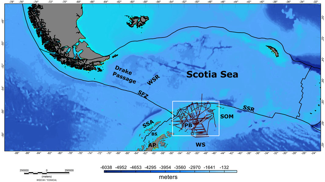
FIGURE 1. Bathymetry map of the Scotia Sea [SRTM30 Plus v7; Becker et al. (2009)] The study area is delimited by a white rectangle. Black lines show the location of MCS profiles used in this study. An elliptical white dotted outline marks Powell Basin’s location. AP, Antarctic Peninsula; BS, Bransfield Strait; PB, Powell Basin, SFZ, Shackleton Fracture Zone; SSR, South Scotia Ridge; SOM, South Orkney Microcontinent; SSA, South Shetland Archipelago; WS, Weddell Sea; WSR, West Scotia Ridge.

The Powell Basin is an elliptically shaped basin characterized by a smooth topographic relief that varies from 3,000 to 2,400 mbsl (Figure 1). The basin is surrounded by continental crust, to: the north by the South Scotia Ridge (SSR), to the east by the South Orkney Microcontinent (SOM), and to the west by the Antarctic Peninsula (AP). Its southern limit is a bathymetric ridge that delineates the northern part of the Weddell Sea.

The tectonic history of the Powell Basin is still poorly understood despite, numerous efforts on the basis of seismic reflection data and one profile of seismic refraction experiment carried out in its northern part its oceanic nature was established by King et al. (1997). Coren et al. (1997) proposed a three-phase evolution process: 1) A rifting phase that started ca. 27 Ma followed by 2) an asymmetric spreading between the eastern and western margins active up to 18 Ma and causing 3) a 11° clockwise rotation of the SOM block that finished in the Early Pliocene. Other models (Rodriguez-Fernandez et al., 1994; Eagles and Livermore, 2002), based on multichannel seismic data and patterns of magnetic reversal, proposed a two-phase tectonic evolution: rifting and spreading. However, there is no agreement on the start and duration of the spreading phase. Rodriguez-Fernandez et al. (1994) proposed the oceanic spreading occurring between late Eocene (∼38–34 Ma) and early Miocene (23–20 Ma) whereas Eagles and Livermore (2002) support that the spreading occurred between 29.7 and 21.8 Ma.

In addition, to the tectonic evolution, the extent of the spreading is also a subject of debate. Some authors (Rodriguez-Fernandez et al., 1994; King et al., 1997; Eagles and Livermore, 2002) support a wide extent of the newly created oceanic crust that would occupy a large portion of the basin. In contrast, Coren et al. (1997) estimated that the spreading area is concentrated in an elliptical-shaped zone located to the north of the basin, while the zone located to the south would be formed by an extended continental crust. Catalán et al. (2020) performed a comprehensive study of the basin based on magnetic anomaly analytical signal information, Bouguer gravity anomaly and total tectonic subsidence analysis. In this study, the authors identify the different tectonic boundaries during the formation of Powell Basin from the beginning of the rifting until the end of the oceanic spreading. It helps defining the nature of the crust in the northern, eastern and western margins of Powell basin as: extended and thinned continental crust, intruded and thinned continental crust, and oceanic crust, respectively. According to their results, the extension of the oceanic seafloor is smaller than proposed by previous studies (Rodriguez-Fernandez et al., 1994; King et al., 1997; Eagles and Livermore, 2002), but larger than the extension proposed by Coren et al. (1997).

Seafloor spreading magnetic alignments have been key to the development of the Plate Tectonics Theory. They are caused mainly by the extrusive basaltic layer. The amplitude of these anomalies depends on the remnant magnetization amplitude that oscillates between 20 and 3 A/m (Gee et al., 1994; McElhinny and McFadden, 2000). The depth of the seabed, which acts as a low-pass filter, also conditions the amplitude. Visualizing marine magnetic profiles of different oceanic basins, and taking 3,000 m depth, the average seafloor depth at Powell Basin as an arbitrary reference, it is easy to find amplitudes larger than 150 nT and even 400 nT (peak to peak) at the mid-Atlantic ridge area.

Several authors highlighted the presence of low amplitude magnetic anomalies in Powell Basin (40 nT peak to peak) (King et al., 1997; Eagles and Livermore, 2002). Some studies suggested that the proposed anomalies could be suppressed because of hydrothermal circulation system within the upper crust that is confined by overlying low permeable sediments preventing fluids venting directly into the overlying cold seawater. This retention of hot fluids would have caused leaching of iron oxides, reducing the amplitude of magnetic anomalies (Levi and Riddihough, 1986).

To isolate and detect seafloor spreading magnetic anomalies in Powell Basin and to better understand the nature of the basin as well as the geodynamic processes in the area, Catalan et al. (2020) performed an analysis of the abnormal low amplitude of Powell Basin’s magnetic anomalies. These authors detected an area where the amplitudes were smaller (by a factor of 2) than in the rest of the basin. They found the existence of a spatial correlation between this area and an asthenospheric branch coming from the Scotia Sea proposed by Martos et al. (2019). In this study, the authors proposed a horizontal heat flow distribution in the Scotia Sea [Figure 4A in Martos et al. (2019)] and surrounding regions and concluded that the heat flow map is consistent with a Pacific mantle flow towards the Atlantic through the Scotia Sea where the SFZ plays an important role as asthenospheric barrier. Based on the previous results, Catalan et al. (2020) support the effect of heat injection of the Pacific mantle outflow in the magnetic anomaly signature of Powell Basin.

Geothermal heat flow provides information regarding the thermal state of the lithosphere. Lawver et al. (1994) performed six measurements during a campaign on board the R/V “Nathaniel B. Palmer”. Reported values vary between 74 and 83 mW/m² with a maximum value of 96 mW/m² located near an extinct spreading center. Nagao et al. (2002) presented a regional survey of heat flow measurements carried out on board the R/V “Hakurei” around in Antarctica. Only two measurements were collected in Powell Basin. More recently, Dziadek et al. (2021) studied three different geological areas (Weddell Sea and Antarctic Peninsula, Powell Basin, Aurora Vent field and Western Gakkel Ridge) using thermal observations. This study discussed the thermal structure of Powell Basin using Lawver et al. (1994) and Nagao et al. (2002) data as well as eleven new heat flow measurements from an expedition on R/V “Polarstern” in 2021. On this survey 10 out the 11 heat flow measurements were collected in the northwestern part of the basin and one isolated station in the western part. Dziadek et al. (2021) compared all these heat flow values in the oceanic crust domain with global models and concluded that they are within the predicted normal range for an ocean of ∼30 Ma.

The “ElGeoPoweR” expedition to study Powell Basin was carried out on board the R/V “Sarmiento de Gamboa” in January 2022. During this campaign new magnetic field measurements were collected along with systematic geothermal heat flow values following a regularly spaced transect across the basin (Figure 2A).

FIGURE 2

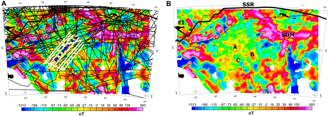
FIGURE 2. (A) Magnetic track line dataset of the study area. In thick white lines tracklines obtained through “ElGeoPoweR” cruise. Blue circles denote the location of heat flow measurements from ElGeoPoweR cruise. (B) Magnetic map of the area at 5 km resolution. A thin solid black line surrounds the Pacific Margin Anomaly (PMA). A dotted line highlights some features (see text for explanation). SSR, South Scotia Ridge; SOM, South Orkney Microcontinent; EI, Elephant Island. Labels “A”, “B” and “C” highlight three magnetic anomalies (see text for explanation).

The objectives of the present work are to shed light into 1) the thermal state of Powell Basin and its lateral variability, 2) the observed low amplitude magnetic anomalies, and 3) the potential existence of the Pacific mantle outflow branch flowing in this region. For this, we study the magnetization, the Moho discontinuity and geothermal heat flow of Powell Basin making use of magnetic, gravity and geothermal heat flow data, most of them obtained during “ElGeoPoweR” expedition.

Here, we provide an explanation that supports the presence of a moderate level of magnetization in some places as well as areas with a small value in magnetization.

2 Data and methods

For this study, we used magnetics, gravity, heat flow, bathymetry and sediment thickness derived from multichannel seismic cross sections. Below we describe technical aspects related to the data collection, sources used and the methods applied in our study.

2.1 Magnetic data

Data from a compilation of marine magnetic anomalies (Quesnel et al., 2009) served as the basis to produce the second version of the World Digital Magnetic Anomaly Map (Lesur et al., 2016). This database uses the CM4 model to remove the internal and external field contributions (Sabaka et al., 2004). The database was cleaned, and spikes were removed. To reduce inconsistencies between lines we have leveled the entire database (Figure 2A, in solid black).

Additionally, we included data from eight Spanish marine surveys carried out on board R/V “Hespérides” between 1992 and 2013, and data acquired during the “ElGeoPoweR” cruise aboard R/V “Sarmiento de Gamboa” (Figure 2A, white lines). To remove the internal magnetic field contribution, all tracks were corrected using the International Geomagnetic Reference Field IGRF 13 (Alken et al., 2021). To remove the external fields contribution during “ElGeoPoweR” cruise and the rest of Spanish marine surveys carried out on board R/V “Hespérides” between 1997 and 2013, we used the Livingston magnetic observatory data. The Spanish 1992 cruise was corrected using the CM4 model. Finally, we used all the previously cited magnetic data to obtain a map of magnetic anomalies with a resolution of 5 km at sea level (Figure 2B).

2.2 Bathymetry data and sediment thickness data

Bathymetry was obtained using the SRTM30plusv7 grid (1 km resolution) (Becker et al., 2009). For sediment thickness we used multichannel seismic data obtained in the Powell Basin and its surroundings extracted from the Seismic Data Library System. These profiles were used in Catalán et al. (2020). Technical information regarding data collection and processing are included in that publication.

2.3 Heat flow data

To better constrain the thermal structure of Powell Basin and contribute to the rather small existing heat flow data base in this region, we acquired ten heat flow measurements using a violin bow-type probe. The probe functionality is based on the principles described in Hartmann and Villinger (2002). The equipment is both mechanically robust to withstand repeated insertions and withdrawals from the seafloor and highly accurate. The instrument contains an array 6 m-long of 22 thermistors of 1 mK precision. The standard heat flow acquisition workflow is as follows: The heat flow probe is lowered and inserted into the seabed by its own weight. This generates a frictional heat pulse that dissipates in the surrounding sediment. Ten minutes after the insertion, a second, 20 s long, calibrated heat pulse of 1 kJ/m is released by the probe. The decay of both pulses is recorded into marine-grade solid-state memory by custom microcontroller-based hardware and embedded software. When the probe is recovered and the time series retrieved from memory, equilibrium temperatures for each thermistor are then calculated by fitting the frictional pulse time series to a cylindrical decay curve over a 10-min time window. Finally, the temperature decay of the calibrated pulse is used to estimate the in situ thermal conductivity (Hartmann and Villinger, 2002).

Ten heat flow measurements were collocated with bathymetric information and magnetic profiles acquired during the cruise (Figures 2A, 3A: blue circles) and spaced unevenly between 33 and 9 km across the Powell Basin (Figure 4A). Even though the sampling strategy focused on areas with a sediment cover thick enough to facilitate the probe insertion, the sediment cover in the central rise area was thin and coarse but penetrations consistently reached 5.25 m for most stations. On the flanks of the basin, conditions were worse, achieving partial penetrations only.

FIGURE 3

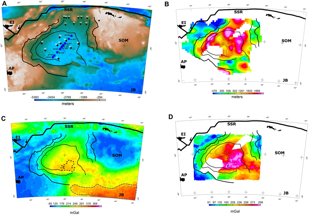
FIGURE 3. (A) Bathymetry map of study area. Blue circles depict location of heat flow measurements from ElGeoPoweR cruise. In black inverted triangles data collected from R/V “Polar Stern”. Black diamonds denote the location of data collected from R/V “Nathaniel B. Palmer”. Black squares denote the location of data collected from R/V “Hakurei”. White numbers indicate heat flow readings in mW/m². (B) Sediment thickness map of the study area. We have included only the area where MCS coverage is adequate. (C) Complete Bouguer gravity anomaly map. A black dotted line surrounded the largest complete Bouguer gravity anomaly values in the basin. A grey dashed polygon highlights an E-W Complete Bouguer gravity anomaly. (D) Complete Bouguer gravity map after subtracting the sediment gravity contribution. At (B) and (D) a black dotted curvilinear polygon highlights a NW-SE alignment which divided the whole basin into western and eastern parts. At (B) and (D) the northern part of this dotted polygon is in green (see text for clarification). AP, Antarctic Peninsula; JB, Jane Bank; SSR, South Scotia Ridge; SOM, South Orkney Microcontinent; EI, Elephant Island. Thick and thin black lines delimit extended continental crust, thin and dotted delimits extended and intruded continental crust domains. A black dotted line delimits the outer boundary of the ocean domain according with (Catalán et al., 2020). At (C) and (D) label “C” highlights a Bouguer gravity anomaly high.

FIGURE 4

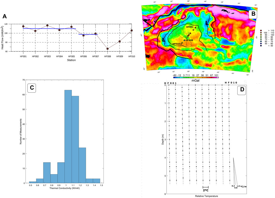
FIGURE 4. (A) Heat flow measurements taken along the transect at Powell Basin. Two blue lines marks the average values for the first and for the second intervals (see text for comments). (B) Free-air gravity anomaly map. Heat flow measurements are shown in color-coded circles following the scale bar displayed at the right of the figure. HF001 at the NE location while HF010 at the SW. A black dotted curvilinear polygon highlights a NW-SE magnetization alignment, which divided the whole basin into western and eastern parts. Two linear lows in its western and northeastern margins are label as “L”. Thick and thin black lines delimit extended continental crust; thin and dotted delimits extended and intruded continental crust domains. A black dotted line delimits the outer boundary of the ocean domain according with (Catalán et al., 2020). (C) Histogram showing the thermal conductivity for the transect across Powell Basin. The mean thermal conductivity over the transect is 1.05 W m⁻¹ K⁻¹ and its standard deviation is 0.15 W m⁻¹ K⁻¹. (D) Temperature-depth profiles across the Powell Basin. HF001 at the leftmost, HF010 at the rightmost position. Profiles were obtained using a violin-bow system of 22 thermistors along a thermistor string 6 m long. For partial penetrations, the poor model fit precludes the interpretation of these measurements. Temperature gradients present a linear tendency, which is indicative for thermally stable conditions.

2.4 Gravity data

2.4.1 Free air gravity anomaly, complete Bouguer gravity anomaly and Moho discontinuity

We have used the global free air dataset from Sandwell et al. (2014) with a resolution of 1 mile (Figure 4C) to mark the extinct ridge axis and its limits. Complete Bouguer gravity anomalies were calculated following Nettleton (1976) procedure. We have removed water slab and seafloor topography gravity contribution and apply terrain corrections. Further details regarding gravity data treatment are included in Catalán et al. (2020). Finally, we obtained a Complete Bouguer anomaly grid with 2 km resolution (Figure 3C).

As the seismic lines coverage is not optimal and present gaps in the southwestern area of Powell Basin, we calculated a sediment thickness grid only where this information is available. A complete Bouguer anomaly map not affected by the sediment thickness gravity contribution is helpful and will be used in the discussion (Figure 3D). To compute its gravitational effect and extract it afterwards, we used the full Parker’s method (Parker, 1972). For this we used a value of 2,100 kg/m³ of density inferred from the average velocity model as function of depth provided by King et al. (1997) and we have used the density-velocity relationship provided by Gardner et al. (1974).

The crustal structure of the basin is poorly known as there is only one line of seismic refraction experiment carried out in its northern part. Therefore, to derive the Moho’s undulating boundary (MUB) we used observed gravity data by gravity inversion we followed Chávez et al. (2007) and used the complete Bouguer anomaly map for this purpose. We have not used the complete Bouguer anomaly map corrected by the sediment thickness gravity contribution, as there is not adequate control on the sediment thickness in the whole basin.

For the inversion process to estimate the MUB we used the LithoFLEX software (Braitenberg et al., 2007). We used 13.5 km as reference depth, and a value of 500 kg/m³ as density contrast between the crust and the mantle following Chávez et al. (2007). Finally Figure 5 describes the depth to the MUB. In order to facilitate the convergence of the inversion of the gravity grid, we selected a square map centered on Powell Basin which extends slightly laterally to guarantee a stable solution over the basin, minimizing any possible edge effects in the study area.

FIGURE 5

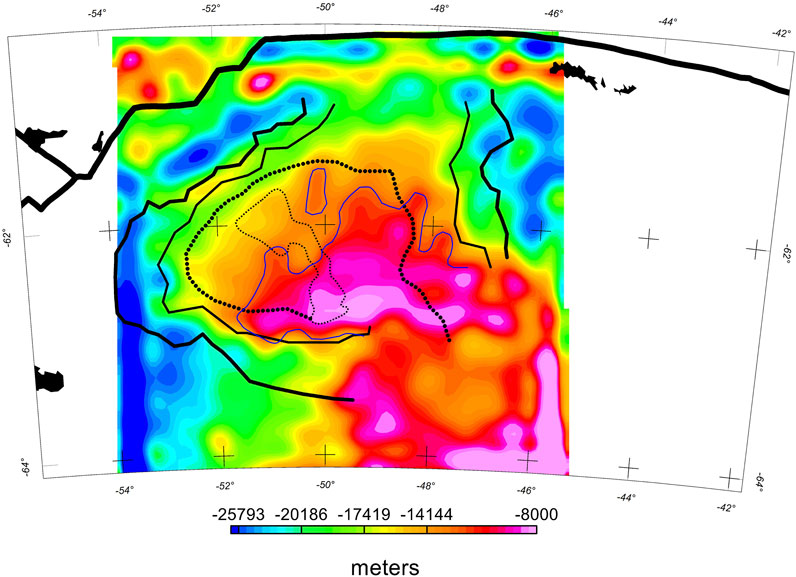
FIGURE 5. 3D geometry of the MUB. Model obtained by inversion of the regional gravity anomaly data (Figure 3C). Thick and thin black lines delimit extended continental crust, thin and dotted delimits extended and intruded continental crust domains. A black dotted line delimits the outer boundary of the ocean domain according with (Catalán et al., 2020). A thin blue line delineates the 13.3 km-isoline. A black dotted curvilinear polygon highlights a NW-SE magnetization alignment, which divided the whole basin into western and eastern parts.

2.5 Equivalent magnetization method

A magnetic anomaly map shows the horizontal distribution of magnetic properties of the lithosphere. This picture is conditioned by factors such as the irregular shape of the ocean floor that can produce large anomalies masking other important magnetic signals. It is also conditioned by geographical location since the Earth’s magnetic field is a vector. To correct the magnetic anomalies for the effects introduced by the topography of the ocean floor, and for the phase shift due to latitude, we have used the three-dimensional inversion method of Parker and Huestis (1974). We assume an inclination of −55° for the geomagnetic vector according to what is predicted by the International Geomagnetic Reference Field (IGRF) model for the study area. The upper boundary is defined by the topography of the ocean floor, and the lower boundary is located 500 m below this topography. To ensure the convergence of the inversion we have used a band-pass filter with upper and lower cut-off wavelengths set at 100 and 5 km, respectively. This allows us to resolve short wavelengths signals that correspond to the most superficial part. To appreciate more clearly the distribution of the variation of the equivalent magnetization, we obtained a grid that results from considering the absolute value only of the short wavelength (from 100 to 5 km) magnetization map. These values will be called hereafter magnetization amplitude.

As we want to highlight large variations in the magnetization map, and attenuate any local effects (i.e., topography), we have also applied a low-pass Butterworth filter of order 9, and we have set 30 km as the cut-off wavelength after an iterative process of trial-and-error until the result shows no noise and only smooth variations (Figure 6A).

FIGURE 6

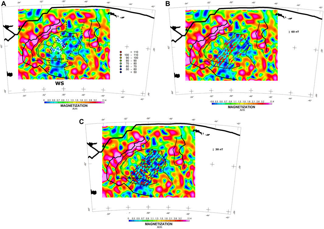
FIGURE 6. (A) Low-pass filtered crustal magnetization amplitude map of the study area (see text for explanation). Heat flow measurements are shown in color-coded circles following the scale bar displayed at the right of the figure. HF001 at the NE location while HF010 at the SW. A red dotted line delineates a plausible limit for the oceanic boundary at the SE of the oceanic basin. A black thin dotted curvilinear polygon highlights a NW-SE magnetization alignment, which divided the whole basin into western and eastern parts. A black curvilinear polygon delineates the area where the highest amplitudes of magnetization values (>1.5 A/m) are located. WS, Weddell Sea. Two white thin dotted polygons delimit two areas with low magnetization (even null) values. Two thick brown square dotted lines limited the proposed path followed by the asthenospheric branch inside the Powell Basin. (B) A wiggle plot showing original magnetic anomaly profiles along Powell Basin. (C) A wiggle plot showing magnetic anomaly profiles high pass filtered (50 km cut-off wavelength) along Powell Basin. In (A), (B) and (C) thick and thin black lines delimit extended continental crust, thin and dotted delimits extended and intruded continental crust domains. A thick black dotted line delimits the outer boundary of the ocean domain according with (Catalán et al., 2020).

3 Results

3.1 Magnetic anomaly map

After compiling the magnetic field data including the new profiles and performing leveling, we observed that the northern and eastern part of the Powell Basin are characterized by magnetic anomalies highs (Figure 2B). These anomalies correspond to the Pacific Margin Anomaly (PMA), which runs sub-parallel to the Pacific margin of the Antarctic Peninsula (Garrett, 1990; Suriñach et al., 1997; Ghidella et al., 2002; Martos et al., 2014a). The PMA is considered a linear batholithic complex related to a Mesozoic-Cenozoic magmatic arc, which runs along the Pacific-Antarctic margin until it reaches the Bransfield Strait where it splits into two branches, one running along the South Shetland Archipelago block, and the other one running roughly sub-parallel along the northern margin of the Antarctic Peninsula (Catalán et al., 2013).

Regarding the magnetic anomaly map used in Catalán et al. (2020), the new map (Figure 2B) shows differences mainly in its central area due to the inclusion of the new lines from the “ElGeoPoweR” Antarctic survey. This area shows a NW-SE linear structure interrupted in its central part, splitting into two pieces with an “J-like” shape” in the NW, and another in the SE (Figure 2B: labeled as “A” and “B” respectively). The southern east margin includes a magnetic anomaly delimited by a dotted line in Figure 2B, which surrounds the SOM’s southern margin toward the east. This margin was interpreted by Rodríguez-Fernández et al. (1994) as a structural ridge between the Powell Basin and the Weddell Sea.

3.2 Complete Bouguer gravity anomaly map

The Complete Bouguer gravity anomaly map shows a simple picture (Figure 3C). The central part of the basin presents high values (larger than 240 mGal) probably related to the oceanic character of the crust in this area. The smallest amplitude values are in the western and eastern part, related to the AP and the SOM, respectively, as continental areas. The central part of the basin presents an anomaly high that extends linearly towards the SE linking with an E-W anomaly corresponding to the Jane Bank (Figure 3C, delimit by a grey dashed polygon). Label “C” marks the presence of a Bouguer gravity anomaly high (Figures 3C, D).

3.3 Equivalent magnetization map

The magnetization amplitude map (5–100 km) (Figure 6A) shows a distribution of values ranging from 0 to 11.4 A/m. These values are distributed in such a way that the largest ones surround the basin in the East and in the West. These areas correspond to the location of the PMA. Towards the south there are large magnetization values. They correspond to the margin interpreted by Rodríguez-Fernández et al. (1994) as a structural ridge between the Powell Basin and the Weddell Sea.

Inside the basin the magnetization amplitude is smaller than 2 A/m. A NW-SE alignment of values that range between 0.7 and 1.1 A/m divides the whole basin into a western and an eastern part (Figure 6A: inside a black dotted curvilinear polygon). The highest value (>2 A/m) is located to the northwest of the western area. Along the rest of this part, values range between 1 and 2 A/m (Figure 6A: inside a solid black curvilinear polygon). On average the eastern part presents the lowest values (<1 A/m).

3.4 Heat flow measurements

The ten heat flow measurements collected in Powell Basin during the campaign and its associated uncertainties are included in Table 1. Once corrected by the effect of sedimentation (e.g., Neumann et al., 2017), they range between 66 and 117 mW/m² (Table 1). The mean thermal conductivity over the transect is 1.05 W m⁻¹ K⁻¹ and its standard deviation is 0.15 W m⁻¹ K⁻¹ (Figure 4C). Temperature-depth profiles for heat flow measurements in the Powell Basin transect are shown in Figure 4D. Stations HF001-HF010 show linear temperature gradients, which are indicative for thermally stable conditions.

TABLE 1

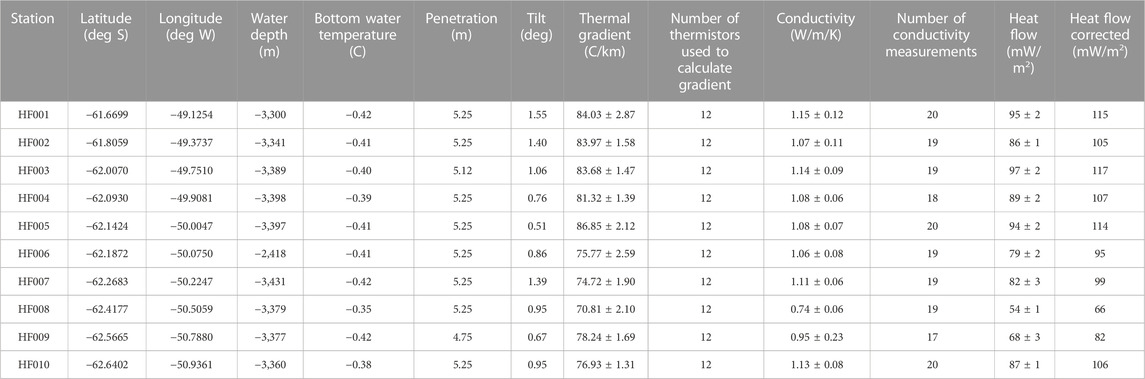
TABLE 1. Results of geothermal heat flow from 2022 Powell Basin survey obtained after R/V “Sarmiento de Gamboa” cruise.

In heavily sedimented environments, heat flow is depressed because of the delay required to warm cold sediments to the background thermal conditions. Sedimentation rates in Powell Basin are not precisely known but age models (Lindeque et al., 2013) suggest sediment accumulation rates of ∼0.104, 0.108, and 0.07 mm/yr for Pre-Glacial, Transitional and Glacial units respectively. Furthermore, these authors predict that Powell Basin has accumulated a total of 2,227 m of sediments: 918 m of Pre-Glacial deposits, 625 m of Transitional sequences, and 684 m of Glacial stratigraphic units. All thickness and sedimentation rate estimates were calculated for selected points on a Weddell Sea-Scotia Sea seismic transect (Lindeque et al., 2013). To estimate the impact of sedimentation on heat flow we used the one-dimensional transport-diffusion equation, assuming a sedimentation rate of 0.07–0.1 mm yr⁻¹ over the past 24 Myr (Powell et al., 1988). The solution to this equation indicates a maximum suppression of 21% in heat flow in the central Powell Basin from the currently observed value of 83 ± 13 mW m⁻² to a sedimentation-corrected value of 101 ± 16 mW m⁻².

We identify three segments in the Heat flow values acquired during the ElGeoPoweR campaign. The first segment includes stations HF001 to HF005. This first segment concentrates the highest values obtained throughout the entire profile (with an average value of 112 mW m⁻²). Subsequently, HF006 and HF007 show similar values though somewhat lower than those on the first segment, averaging 97 mW m⁻². Stations HF008, HF009 and HF010 break the previous trend, showing a minimum value of 65 mW/m² at HF008 whereas HF009 and HF010 values increase again following an almost linear trend reaching the same amplitude midway between the average of the first segment and the second segment (Figure 4A). It is noteworthy, that the thermal gradients from HF007 to HF010 are similar with a range between 0.07ºC–0.08ºC/m, however thermal conductivities decrease from around 1.00 to 0.74 W m⁻¹ K⁻¹ for stations HF007 and HF008, respectively. The decrease in thermal conductivity leads to a lower heat flow value at station HF008.

3.5 The extinct spreading axis

The extinct spreading axis was identified by multichannel seismic profiles obtained during the HESANT 92/93 cruise (Rodriguez-Fernández et al., 1994). In these profiles the axis appears split into two ridges separated by a central depression filled with sediments. The free-air gravity anomaly map (Figure 4B) shows a Y-like shaped high runs along the central part of the basin with a W-E and NW-SE trends. The space between these two branches marks the extinct spreading axis (Rodriguez-Fernandez et al., 1994; Eagles and Livermore, 2002). It is a 15 km-wide rift with no exposed basement on the surface (Rodriguez-Fernández et al., 1994; King et al., 1997). This area is where the sedimentary thickness is minimal: 1 km thinner than in the western and eastern parts of the basin (Figure 3B). Over the extinct spreading axis, the magnetization amplitude (Figure 6A) shows values ranging from 1.1 to 1.3 A/m, which is part of a longer NW-SE alignment that will be subject of discussion on section 4.5.

4 Discussion

We perform an integrated analysis of the Powell Basin using gravity, magnetics, heat flow, magnetization and the Moho discontinuity depth model for the basin. To facilitate the discussion it is important to define the state of the art of the basin regarding the low amplitude of the magnetic anomaly. It allows us to locate which areas host these low amplitude magnetic anomalies. To achieve this we use results from previous studies and discuss them with the information derived with our new magnetic anomaly data obtained during our cruise. In this section we analyze different options, which could cause such low magnetic anomaly amplitudes such as the sediment thickness layer or a decrease in the global Earth’s magnetic field intensity. We analyze the results provided by our NE-SW geothermal heat flow transect and highlight how these values evidence the extinct spreading axis’ role as a boundary dividing the basin in three sectors. We find a correspondence between the heat flow measurements and the magnetization values reached throughout the basin. It leads us to analyze the effect of the asthenospheric flow on the magnetic anomaly amplitude. Finally, we discuss the NW-SE magnetization alignment, and how it contributes explaining the magnetization amplitude in the basin.

4.1 Abnormal magnetic anomaly amplitude in Powell Basin

Catalán et al. (2020) discussed the nature and probable origin of small amplitudes of the magnetic anomalies in the Powell Basin. They used profiles from previous marine magnetic surveys crossing the basin [Figure 7 in Catalán et al. (2020)]. These profiles show an area where the amplitudes decreased and ranged between ± 20 nT peak to peak in the north and in the central part of the basin, or between ± 10 nT peak to peak in profiles located in the south and central parts. The orientation of the track lines corresponding to these profiles was not systematic. In contrast, the eight profiles from “ElGeoPoweR” expedition were designed to follow a perpendicular orientation with respect to the spreading axis.

Figure 6B shows a wiggle plot of the original magnetic anomalies acquired during the ElGeoPoweR campaign and an additional wiggle plot (Figure 6C), where data was high pass filtered with a 50 km cut-off wavelength to eliminate regional trends following Catalán et al. (2020) and Eagles and Livermore, (2002). Thus, the magnetic sources causing these filtered anomalies correspond to shallow magnetic bodies.

Figures 6B, C show original low amplitude magnetic anomalies in Powell Basin where the amplitude of magnetization is low or even zero. This confirms that these areas are characterized by true signals and they are not an artifact resulting from the mathematical approach used to compute the magnetization. In Figure 6A we have plotted the boundary proposed by Catalán et al. (2020) for the oceanic crust (the black thick dotted line in Figure 6A) delimiting the magnetization domain which has a clearly different magnetization signature than the surrounding areas. Although Catalán et al. (2020) were unable to delineate the southeast boundary, the amplitude of magnetization suggests a clear limit (See Figure 6A red dotted line). The map in Figure 6A provides a precise image of the location of the areas where the magnetization amplitude is small or almost null, and therefore it provides important clues about their origin.

Figure 6A also shows that the basin is split in two by a 15 km-wide central area with values of ∼1 A/m (a thin dotted black line). The northern part of the thin dotted polygon roughly coincides with the extinct spreading axis. Eastward of this central alignment there are large areas where the values of the magnetization amplitude are zero. In this part, some NE-SW curvilinear alignments show small but not necessarily null magnetization amplitudes (∼1 A/m). Along the western part of the central alignment, there is a branch of zero magnetization amplitude (Figure 6A: inside a white dotted polygon). This branch northerly limits a large area located to the north of the Weddell Sea showing zero magnetization amplitude (laterally limited by the southwardly prolongation of two thick brown square dotted lines).

Eagles and Livermore (2002) and King et al. (1997) attributed the low amplitude of magnetic anomalies to hydrothermal alteration of oceanic basalts beneath sediment-covered spreading centers. However, it is important to note that the whole western part of the basin presents an average value of 0.98 A/m, while in the East the average magnetization amplitude is only half of that in the west (0.47 A/m). This lack of symmetry leads us to question the idea of hydrothermal circulation, as we would expect an equal influence on both sides of the extinct spreading axis (central magnetization alignment) according with Eagles and Livermore (2002) which proposed a symmetric spreading rate along Powell Basin opening history (29.7–21.8 Ma).

4.2 Sediment layer contribution. Distance from the magnetic source

Catalán et al. (2020) discuss the possibility that a ∼2 km thick sedimentary layer could cause at least some attenuation that locally affects the amplitude of magnetic anomalies. The basin shows uniform seafloor topography, ranging between 5,100 and 5,500 m (Figure 3A). Sediment thickness at the eastern part ranges from 1940 to 2,300 m (Figure 3B). According with that the basement topography is rather uniform, ranging from 7,000 to 7,800 m. Regarding the western part we cannot say anything conclusive due to the lack of seismic data. However, the complete Bouguer map shown in Figure 3C shows that the gravity response of the western area is mostly composed of long wavelength signals (Figure 3B), which denotes a rather uniform basement topography similar to the eastern area.

Figure 6A shows the presence of several northeast-southwestward magnetization curvilinear alignments at the eastern side, the area most affected by the attenuation of the magnetic anomaly amplitude. This alignment shows no correlation with the sediment cover (Figure 3B). As seafloor topography is uniform, it means that there is no correlation with the basement topography.

4.3 A decrease in the global Earth’s magnetic field intensity

A possibility to understand the weakening in the amplitude of the magnetic anomalies could be a temporary decrease in the Earth’s magnetic field paleointensity.

Tivey and Johnson (1987) discussed the possibility that a sudden worldwide geomagnetic intensity increase was able to produce the required near-axis magnetization contrast at the Central Anomaly Magnetization High anomaly. Following Klitgord et al. (1975) studies on magnetization solutions from near-bottom profiles over six ridge segments in the East Pacific, and Prévot and Grommé (1975) studies comparing the mean intensity of magnetization of submarine basalts from the North Atlantic with the intensity of subaerial basalts. They argued that Paleointensity variations require changes that are too large compared with the current best estimates of recent geomagnetic field variations.

Besides, at ordinary seafloor spreading the ridge plays a key role to evidence a roughly symmetrical process where the decrease in M should be reflected on both sides of the extinct ridge axis. This is not observed at Figure 6. This is supported too observing the distribution of the magnetic anomaly amplitudes on both sides of the ridges (Figure 6C: wiggles). Figure 6C shows three- or five-fold amplitudes on its western side when compares with its eastern side.

Therefore, we conclude that the weakening detected in the amplitude of the magnetic anomalies in the Powell Basin does not respond to a decrease in the Earth’s magnetic field but to a specific process in our study area.

4.4 Geothermal heat flow and magnetization evolution controlled by asthenospheric flow

From all the heat flow measurements collected on previous cruises (Lawver et al., 1994; Nagao et al., 2002; Dziadek et al., 2021), only those made by Lawver et al. (1994) were relevant for this study and are in good agreement with those acquired during the ElGeoPoweR cruise (Figure 3A). Their values are, however, slightly lower than those obtained in ElGeoPoweR expedition by ∼ 10 mW/m² (except for the observed value of 96 mW/m²). This can be attributed to several effects but, unfortunately, Lawver et al. (1994) did not provide any information regarding the measurement procedure, corrections performed, or error estimates. Therefore, they will not be further considered in our discussion. Our new heat flow measurements confirm that the extinct spreading axis (or central magnetization alignment) is a boundary dividing the basin in three parts: a) The NE region which includes the highest heat flow values with very low or null values of amplitude of magnetization (Figure 3A), b) the extinct spreading axis characterized by intermediate heat flow readings (13% lower than the average value obtained in the previous area), and c) an area located on the western edge of this extinct spreading axis. The lowest value recorded on the survey: 66 mW/m² (Figure 4B: HF008) is located in the limit between b) and c). In contrast, HF009 and HF010 show values that increase westward, reaching in the last measurement a similar value to those obtained in the NE region (>100 mW/m²). Catalán et al. (2020) proposed the presence of an asthenospheric stream, which flows from the Pacific into the Atlantic Ocean through the Drake Passage and into the Powell Basin (Martos et al., 2014b; Martos et al., 2019) to explain the small amplitude of the magnetic anomalies. Magnetic anomalies are a consequence of the magnetic properties of rocks, and they have dependence with temperature. Rocks lose their magnetic properties as temperature increases with depth. This is known as the Curie depth. This depth could be deeper or shallower depending on the activity of the geological/geodynamic environment.

It is commonly accepted that the magnetic response of the oceanic crust is due to the contribution of two layers: one formed by extrusive basalts (<1 km thick) in which the main component is titanomagnetite. It is the main contributor to the striped marine magnetic anomaly patterns. Another layer (∼5 km thick) is formed by gabbro, dolerite, and, in some cases, serpentinized peridotites. Its main component is magnetite (Dunlop and Özdemir, 1997). Extrusive basalts and gabbros have different Curie temperatures. Titanomagnetite has a Curie temperature range between 100ºC–550°C depending on the degree of oxidation (Zhou et al., 2001), while for magnetite it is 580°C.

Here, we propose that the small amplitude of magnetic anomalies is the result of the dependency of rocks’ magnetic properties on temperature. In particular, the extrusive basalt layer that covers this area. The asthenospheric stream penetrates the Powell Basin through its northern area (Martos et al., 2019; Catalán et al., 2020) and would act as an additional heat source affecting the magnetic properties and weakening the anomalies and magnetization.

This is supported by the existence of a correspondence between the heat flow measurements and the magnetization values reached throughout the basin. The area where the maximum heat flow measurements are reached (HF001-HF005) correspond to the eastern part where the magnetization amplitude is very low or practically null. Similarly, heat flow measurements HF009 and HF010 correspond to values that increase westward, reaching HF010 a similar value to those obtained in the NE region. In this area, once again, the amplitude of magnetization reaches practically null values to the south.

The thermal perturbation effect of the previous cited asthenospheric stream is not homogenous throughout the basin. Geothermal heat flux readings located on the extinct ridge axis position mark intermediate values, in coincidence with a slight reinforcement in the value of the magnetization amplitude. We propose that thermal perturbations mainly affect the most exposed areas, varying with the Curie Depth location, which in turn is conditioned by the MUB depth. A similar scenario has recently been reported to occur in the south-easternmost part of the Phoenix Plate (Catalán and Martos, 2022).

To demonstrate the impact of a change in crustal thickness on the temperature within the first kilometer of the crust, we constructed a simple three-layer conductive heat model to test two different scenarios: one with a crustal thickness of 13.5 km and another with 8.5 km. In both cases, the sediment thickness remained constant at 1.5 km. The thermal conductivity values assigned to the three layers were typical for each layer (k = 1.14 W/mK, k = 2.01 W/mK, and k = 5.5 W/mK) (Grose and Afonso, 2019; Lösing et al., 2020; Dziadek et al., 2021). In this model, the temperature at the base (located at 19 km depth) was set at 800°C after extrapolating results from Martos et al. (2019) at depths of 13–14 km in the southern area of the Scotia Arc.

According to our model, a crustal thickness of 8.5 km (Figure 5, estimated crustal thickness in the eastern area) would result, within the 1 km layer of extrusive basalts, in temperatures ranging from 133°C in its uppermost zone, to 191°C (at its base).

In contrast, our model predicts that if the crustal thickness were increased by 5 km to 13.5 km (Figure 5, our estimated crustal thickness in the extinct spreading axis), the temperature provides a temperature range that is well-below 100°C from the top till the base of the extrusive basalt layer. This estimate suggests that in the central part of the basin practically all the layers contribute with their maximum M, while in the Eastern area the lower part reaches the Curie Temperature, and the intermediate layers from the top contribute with a lower (attenuated) M.

This result supports the difference in M values between two areas: central and eastern. Central area whose average M value is 1.53 A/m, and Eastern area, whose average M value is 0.9 A/m (58% of central area average).

Summarizing, according to our models, a 5 km-crustal thickness increase plays a key role to explain the M picture of the Powell Basin. This behavior implies a variation in the contribution of M for every layer. It ranges between 75% and 0% of its saturation value depending on temperature according with Dunlop and Özdemir (1997). However, the contribution of other factors such as pervasive hydrothermal reactions cannot be ruled out.

4.5 The NW-SE magnetization amplitude alignment

Figure 3C shows the largest complete Bouguer gravity anomaly value is ∼273 mGal (labeled as C), which is located in the SE part of the basin (surrounded by a black dashed line). This location coincides with an isolated magnetic anomaly (Figure 2B: same label).

A gravity inversion model predicts that the crustal thickness of this area is extremely thin, and on the order of 8.5 km (Figure 5). The MUB depth values progressively increase up to 14 km towards the NW. The previous section showed that the thermal effect of the asthenospheric flow is strongly conditioned by the topography of the MUB as the Curie isotherm is reached at different depths. Consequently, the greatest attenuation on magnetic anomaly amplitudes should be concentrated in the southeastern part. Figures 6B, C confirm this hypothesis.

The NW-SE magnetization alignment deserves particular attention as it divides the basin into two and approximately coincides with the location of the extinct sperading axis. We propose that this magnetization alignment is the result of two different contributions: a) the magnetization associated with a body with magnetic properties (Figure 2B, label “C”) and, b) the magnetization associated with the extinct ridge axis (Figures 3B, D: in dotted green). Regarding the former contribution, we identify a maximum of the Bouguer gravity anomaly at this location as is shown in Figures 3C, D after the sedimentary layer contribution has been removed. We propose that the increase in the magnetization in this area is produced by the most superficial part of this crustal high-density body. For the extinct ridge axis, according to our interpretation, this is a 15 km-wide spreading with no exposed basement on the surface (Rodríguez-Fernández et al., 1994; King et al., 1997) that could cause the observed increase in magnetization (Figures 6A, 3B). Therefore, it must be a crustal body, however, we do not rule out a contribution from a structural high in the basement that could partially explain it, as the sedimentary thickness layer is thinner along the NW-SE magnetization alignment compared to the rest of the basin (∼1 km).

Tivey and Johnson (1987) pointed out the global occurrence of the central magnetic anomaly high (CAMH) overlying many of the world’s mid-ocean spreading centers. The magnetic contrast associated with the CAMH is in part derived from low-temperature oxidation of the uppermost extrusive volcanic layer assisted by the systematic ridge parallel cracking. Other options exist to justify this increase in magnetization. Guadalupe Island off Baja California, a volcanic island still shows active volcanism 11 million years after the spreading between the Pacific and Guadalupe plates demise (Michaud et al., 2006). A similar situation occurs at the Hellas and Styx seamounts over the Wharton Basin SW of Sumatra (Hébert et al., 1999), or at the Raman and Panikar seamounts in the Lakshmi Basin off Western India (Krishna et al., 2006). All of them are examples of edifices volcanic growth after cessation of the seafloor spreading. This extra magmatism generally forms a locally thicker basaltic crust and justify a reinforce in the magnetization.

Heat flow measurements obtained during the “ElGeoPoweR” Antarctic survey support these possibilities. Values were non-uniform away from the ridge axis (Figures 4A, 6A: HF008 and HF009), while the rest of the measurements (HF001-HF005 and HF010) could be the result of the thermal perturbation caused by the asthenospheric flow overriding any other contribution.

Additionally, the complete and corrected Bouguer gravity map shows a weakening of ∼15 mGal over the extinct spreading axis (Figure 3D: highlighted in green along a black dotted curvilinear polygon). This could indicate a slight crustal thickening along the axis. Furthermore, the 13.3 km-MUB isoline in this part (Figure 5: thin blue line) shows a SE regression, supporting the existence of a 1-km thickening in the expansion zone of the axis that could have allowed the retention of a certain amount of magnetization (values of 0.9 A/m) in the shallowest sources.

In this section we have explored two plausible scenarios that explain the reinforcement of magnetization along the extinct spreading axis: a) the existence of a magnetic crustal body closes to the surface due to a decrease in sediment thickness, and b) a 1 km-crustal thickening that attenuates the loss of magnetization. We propose that it could have been caused by extra magmatism, which after cessation of seafloor spreading, should have formed a locally thicker basaltic crust or from low-temperature oxidation of the uppermost extrusive volcanic layer assisted by the systematic ridge parallel cracking. Available data does not allow a definite conclusion yet, however, we propose that the southern part of the central magnetization high could be the result of the first scenario (a), while the northern part could be caused by a combination of a) and b).

Outside the ridge axis two mechanisms control the variation of the magnetization amplitude along the Powell basin: c) fissuring through hydrothermal alteration mostly affecting the ridge flanks. It competes with d) the demagnetization induced by the Curie isotherm shallowing mainly in the eastern border of the inactive ridge and mostly in the southeast.

Finally, based on the magnetization amplitude map, we can infer the path followed by the asthenospheric branch inside the Powell Basin. According with this map we suggest an inflow through a NE channel and outflow in its SW part (area limited by two thick brown dotted lines at Figure 6A).

5 Conclusion

In this study we have used magnetic, heat flow, bathymetry, gravity, and sediment thickness information to understand the evolution of Powell Basin from the magnetics’ perspective. Here, we presented and evaluated different scenarios that could explain some of the peculiarities of the magnetic anomaly scenario of this basin. The existence of the small-amplitude magnetic anomalies was reported in previous works without any further analysis to explain their origin. Now, our results show that the small-amplitude magnetic anomalies are not widespread but concentrated in the eastern, southwestern and southeastern parts of the basin. Furthermore, we propose that the low magnetic anomaly amplitudes result from the dependency of magnetic properties of rocks on temperature. The asthenospheric branch flow that penetrates the Powell Basin through its northern area proposed by Martos et al. (2019) and Catalán et al. (2020) would act as an additional heat source conditioning a weak magnetic response. The thermal perturbation effect of this flow is consistent with the new heat flow measurements which confirm that the extinct spreading axis (or central magnetization alignment) behaves like a boundary dividing the basin in three parts: 1) the NE region with the highest heat flow values and very low or null values of amplitude of magnetization, 2) the extinct spreading axis, characterized by intermediate heat flow values (13% lower than the average value obtained in the previous area), and 3) the western edge of this extinct spreading axis including the lowest value recorded on the survey. The good correlation between small-amplitude magnetic anomalies and high heat flow values validates our hypothesis: A decrease in magnetization caused by the impact of (1) the astenospheric flow and (2) the lateral variations of crustal thickness. Both control the temperature in the first kilometer of the oceanic crust. Although the contribution of other factors such as pervasive hydrothermal reactions cannot be ruled out, our results support the role of a branch of the Pacific-into-Atlantic asthenospheric flow on the magnetic anomaly amplitudes in Powell Basin and opens new questions and research directions about the upper mantle dynamics and distribution of asthenospheric currents in the study area.

Data availability statement

Publicly available datasets were analyzed in this study. Data used in this study can be found here: For bathymetry at https://topex.ucsd.edu/WWW_html/srtm30_plus.html. For free air gravity data at https://topex.ucsd.edu/WWW_html/mar_grav.html. For multichannel seismic profiles at https://www.scarorg/data-databases/sdls/. For the magnetic anomaly grid, the Complete Bouguer gravity grid, the low-pass filtered magnetization amplitude grid and the 3D geometry of the Moho’s undulating Boundary at PANGAEA Data Archiving and Publication.

Author contributions

MC, RN and YM drafted the manuscript. MC, YM and AS process the magnetic and gravity data. RN, FN and KF process heat flow data. All authors read and approved the final manuscript. All authors listed have made a substantial, direct, and intellectual contribution to the work and approved it for publication.

Funding

This study has been partially funded through project RTI 2018-099615-B-100 entitles “Estructura Litosférica y Geodinámica de Powell Drake-Bransfield Rift” under the umbrella of the Programa Estatal de I+D+i Orientada a los Retos de la Sociedad of the Spanish Ministry of Science.

Acknowledgments

We would like to acknowledge the assistance of the Captain and crew of the R/V “Sarmiento de Gamboa” during the “ElGeoPoweR” Antarctic expedition. YM also thanks the NASA award 80GSFC21M0002.

Conflict of interest

The authors declare that the research was conducted in the absence of any commercial or financial relationships that could be construed as a potential conflict of interest.

Publisher’s note

All claims expressed in this article are solely those of the authors and do not necessarily represent those of their affiliated organizations, or those of the publisher, the editors and the reviewers. Any product that may be evaluated in this article, or claim that may be made by its manufacturer, is not guaranteed or endorsed by the publisher.

References

Alken, P., Thébault, E., Beggan, C. D., Amit, H., Aubert, J., Baerenzung, J., et al. (2021). International geomagnetic reference field: the thirteenth generation. Earth Planets Space 73, 49. doi:10.1186/s40623-020-01288-x

CrossRef Full Text | Google Scholar

Becker, J. J., Sandwell, D. T., Smith, W. H. F., Braud, J., Binder, B., Depner, J., et al. (2009). Global bathymetry and elevation data at 30 arc seconds resolution: SRTM30_PLUS. Mar. Geod. 32 (4), 355–371. doi:10.1080/01490410903297766

CrossRef Full Text | Google Scholar

Braitenberg, C., Wienecke, S., Ebbing, J., Born, W., and Redfield, T. (2007). “Joint gravity and isostatic analysis for basement studies – a novel tool,” in EGM 2007 international workshop, innovation in em, grav and mag methods: A new perspective for exploration (Netherlands: EAGE Publications). doi:10.3997/2214-4609-pdb.166.b_pp_05

CrossRef Full Text | Google Scholar

Catalán, M., Galindo-Zaldívar, J., Martín Davila, J., M Martos, Y., Maldonado, A., Gambôa, L., et al. (2013). Initial stages of oceanic spreading in the Bransfield Rift from magnetic and gravity data analysis. Tectonophysics 585, 102–112. doi:10.1016/j.tecto.2012.09.016

CrossRef Full Text | Google Scholar

Catalán, M., Martos, Y. M., Galindo Zaldivar, J., Pérez, L. F., and Bohoyo, F. (2020). Unveiling Powell Basin’s tectonic domains and understanding its abnormal magnetic anomaly signature. Is heat the key? Front. Earth Sci. 8, 580675. doi:10.3389/feart.2020.580675

CrossRef Full Text | Google Scholar

Catalán, M., and Martos, Y. M. (2022). New evidence supporting the pacific mantle outflow: hints from crustal magnetization of the Phoenix plate. Remote Sens. 14, 1642. doi:10.3390/rs14071642

CrossRef Full Text | Google Scholar

Chávez, R. E., Flores-Márquez, E. L., Suriñach, E., Galindo-Zaldivar, J., Rodríguez-Fernández, J. R., and Maldonado, A. (2007). Combined use of the GGSFT data base and on board marine collected data to model the Moho beneath the Powell Basin, Antarctica. Geol. Acta 5 (4), 323–336. doi:10.1344/105.000000293

CrossRef Full Text | Google Scholar

Coren, F., Ceccone, G., Lodolo, E., Zanolla, C., Zitellini, N., BonazziI, C., et al. (1997). Morphology, seismic structure and tectonic development of the Powell Basin, Antarctica. J. Geol. Soc. 15, 849–862. doi:10.1144/gsjgs.154.5.0849

CrossRef Full Text | Google Scholar

Dunlop, D., and Özdemir, Ö. (1997). “Rock magnetism: fundamentals and Frontiers,” in David edward (Cambridge: Cambridge University Press), 573.

Google Scholar

Dziadek, R., Doll, M., Warnke, F., and Schlindwein, V. (2021). Towards closing the polar gap: new marine heat flow observations in Antarctica and the arctic ocean. Geosciences 11, 11–19. doi:10.3390/geosciences11010011

CrossRef Full Text | Google Scholar

Eagles, G., and Livermore, R. A. (2002). Opening history of Powell Basin, antarctic Peninsula. Mar. Geol. 185, 195–205. doi:10.1016/s0025-3227(02)00191-3

CrossRef Full Text | Google Scholar

Gardner, G. H. F., Gardner, L. W., and Gregory, A. R. (1974). Formation velocity and density—the diagnostic basics for stratigraphic traps. Geophysics 39 (6), 770–780. doi:10.1190/1.1440465

CrossRef Full Text | Google Scholar

Garrett, S. W. (1990). Interpretation of reconnaissance gravity and aeromagnetic surveys of the antarctic Peninsula. J. Geophys. Res. 95 (B5), 6759–6777. doi:10.1029/jb095ib05p06759

CrossRef Full Text | Google Scholar

Gee, J., and Kent, D. V. (1994). Variations in layer 2A thickness and the origin of the central anomaly magnetic high. Geophys. Res. Lett. 21 (4), 297–300. doi:10.1029/93gl03422

CrossRef Full Text | Google Scholar

Ghidella, M. E., Yáñez, G., and LaBrecque, J. L. (2002). Revised tectonic implications for the magnetic anomalies of the western Weddell Sea. Tectonophysics 347 (1–3), 65–86. doi:10.1016/s0040-1951(01)00238-4

CrossRef Full Text | Google Scholar

Grose, C. J., and Afonso, J. C. (2019). New constraints on the thermal conductivity of the upper Mantle from numerical models of radiation transport. Geochem. Geophys. Geosystems 20, 2378–2394. doi:10.1029/2019GC008187

CrossRef Full Text | Google Scholar

Hartmann, A., and Villinger, H. (2002). Inversion of marine heat flow measurements by expansion of the temperature decay function. Geophys. J. Int. 148, 628–636. doi:10.1046/j.1365-246X.2002.01600.x

CrossRef Full Text | Google Scholar

Hébert, H., Villemant, B., Deplus, C., and Diament, M. (1999). Contrasting geophysical and geochemical signatures of a volcano at the axis of the Wharton fossil ridge (N-E Indian Ocean). Geophys. Res. Lett. 26 (8), 1053–1056. doi:10.1029/1999gl900160

CrossRef Full Text | Google Scholar

King, E. C., Leitchenkov, G., Galindo-Zaldivar, J., Maldonado, A., and Lodolo, E. (1997). Crustal structure and sedimentation in Powell Basin. Geol. Seismic Stratigr. Antarct. Margin, Part 2. Antarct. Res. Ser. 71, 75–93. doi:10.1029/AR071p0075

CrossRef Full Text | Google Scholar

Klitgord, K. D., Huestis, S. P., Mudie, J. D., and Parker, R. L. (1975). An analysis of near-bottom magnetic anomalies: sea-Floor spreading and the magnetized layer. Geophys. J. R. Astr. Soc. 43, 387–424. doi:10.1111/j.1365-246x.1975.tb00641.x

CrossRef Full Text | Google Scholar

Krishna, K. S., Gopala Rao, D., and Sar, D. (2006). Nature of the crust in the Laxmi Basin (14º-20º N), western continental margin of India. Tectonics 25. doi:10.1029/2004TC001747

CrossRef Full Text | Google Scholar

Lösing, M., Ebbing, J., and Szwillus, W. (2020). Geothermal heat flux in Antarctica: assessing models and observations by bayesian inversion. Front. Earth Sci. 8, 105. doi:10.3389/feart.2020.00105

CrossRef Full Text | Google Scholar

Lawver, L. A., Williams, T., and Sloan, B. (1994). Seismic stratigraphy and heat flow of Powell Basin. Terra Antartica 1 (2), 309–310.

Google Scholar

Lesur, V., Hamoudi, M., Choi, Y., Dyment, J., and Thébault, E. (2016). Building the second version of the world digital magnetic anomaly map (WDMAM). Earth, Planets Space 68, 27. doi:10.1186/s40623-016-0404-6

CrossRef Full Text | Google Scholar

Levi, S., and Riddihough, R. (1986). Why are marine magnetic anomalies suppressed over sedimented spreading centres? Geology 14, 651–654. doi:10.1130/0091-7613(1986)14<651:wammas>2.0.co;2

CrossRef Full Text | Google Scholar

Lindeque, A., Martin, Y. M. M., Gohl, K., and Maldonado, A. (2013). Deep-Sea pre-glacial to glacial sedimentation in the Weddell Sea and southern Scotia Sea from a cross-basin seismic transect. Mar. Geol. 336, 61–83. doi:10.1016/j.margeo.2012.11.004

CrossRef Full Text | Google Scholar

Martos, Y. M., Catalán, M., and Galindo-Zaldívar, J. (2019). Curie depth, heat flux, and thermal subsidence reveal the pacific mantle outflow through the Scotia Sea. J. Geophys. Res. Solid Earth 124, 10735–10751. doi:10.1029/2019JB017677

CrossRef Full Text | Google Scholar

Martos, Y. M., Catalán, M., Galindo-Zaldívar, J., Maldonado, A., and Bohoyo, F. (2014a). Insights about the structure and evolution of the Scotia Arc from a new magnetic data compilation. Glob. Planet. Change 123, 239–248. doi:10.1016/j.gloplacha.2014.07.022

CrossRef Full Text | Google Scholar

Martos, Y. M., Galindo-Zaldívar, J., Catalán, M., Bohoyo, F., and Maldonado, A. (2014b). Asthenospheric pacific-atlantic flow barriers and the West Scotia Ridge extinction. Geophys. Res. Lett. 41, 43–49. doi:10.1002/2013GL058885

CrossRef Full Text | Google Scholar

McElhinny, P. L., and McFadden, M. W. (2000) Paleomagnetism continents and oceans. International geophysics series, Amsterdam, Netherlands: Elsevier

Google Scholar

Michaud, F., Royer, J. Y., Bourgois, J., Dyment, J., Calmaus, T., Bandy, W., et al. (2006). Oceanic-ridge subduction vs. slab break off: plate tectonic evolution along the Baja California sur continental margin since 15 Ma. Geology 34, 13–16. doi:10.1130/g22050.1

CrossRef Full Text | Google Scholar

Nagao, T., Saki, T., and Joshima, M. (2002). Heat flow measurements around the Antarctica. Proc. Jpn. Acad. 78, 19–23. doi:10.2183/pjab.78.19

CrossRef Full Text | Google Scholar

Nettleton, L. L. (1976). Gravity and magnetic in oil exploration”. New York, NY: Mac Graw-Hill.

Google Scholar

Neumann, F., Negrete-Aranda, R., Harris, R. N., Contreras, J., Sclater, J. G., and González-Fernández, A. (2017). Systematic heat flow measurements across the Wagner Basin, northern Gulf of California. Earth Planet. Sci. Lett. 479, 340–353. doi:10.1016/j.epsl.2017.09.037

CrossRef Full Text | Google Scholar

Parker, R. L., and Huestis, S. P. (1974). The inversion of magnetic anomalies in the presence of topography. J. Geophys. Res. 79 (11), 1587–1593. doi:10.1029/jb079i011p01587

CrossRef Full Text | Google Scholar

Parker, R. L. (1972). The rapid calculation of potential anomalies. Geophys. J.R. Astr. Soc. 31, 447–455. doi:10.1111/j.1365-246x.1973.tb06513.x

CrossRef Full Text | Google Scholar

Powell, W. G., Chapman, D. S., Balling, N., and Beck, A. E. (1988). “Continental heat-flow density,” in Handbook of terrestrial heat-flow density determination: With guidelines and recommendations of the international heat-flow commission. Editors R. Haenel, L. Rybach, and L. Stegena (Dordrecht: Springer Netherlands), 167–222. doi:10.1007/978-94-009-2847-35

CrossRef Full Text | Google Scholar

Prévot, M., and Grommé, S. (1975). Intensity of magnetization of subaerial and submarine basalts and its possible change with time. Geophys. J. R. Astr. Soc. 40, 207–224. doi:10.1111/j.1365-246x.1975.tb07047.x

CrossRef Full Text | Google Scholar

Quesnel, Y., Catalán, M., and Ishihara, T. (2009). A new global marine magnetic anomaly data set. J. Geophys. Res. 114 (B4), B04106–B04111. doi:10.1029/2008JB006144

CrossRef Full Text | Google Scholar

Rodriguez-Fernandez, J., Balanya, J. C., Galindo-Zaldivar, J., and Maldonado, A. (1994). Tectonic evolution of a restricted ocean basin: the Powell Basin (northeastern antarctic Peninsula). Geodinámica Acta 10 (4), 159–174. doi:10.1080/09853111.1997.11105300

CrossRef Full Text | Google Scholar

Sabaka, T. J., Olsen, N., and Purucker, M. E. (2004). Extending comprehensive models of the Earth’s magnetic field with ørsted and CHAMP data. Geophys. J. Int. 159, 521–547. doi:10.1111/j.1365-246X.2004.02421.x

CrossRef Full Text | Google Scholar

Sandwell, D. T., Müller, R. D., Smith, W. H. F., Garcia, E., and Francis, R. (2014). New global marine gravity model from CryoSat-2 and jason-1 reveals buried tectonic structure. Science 346, 65–67. doi:10.1126/science1258213

PubMed Abstract | CrossRef Full Text | Google Scholar

Suriñach, E., Galindo-Zaldivar, J., Maldonado, A., and Livermore, R. (1997). Large amplitude magnetic anomalies in the northern sector of the Powell Basin, NE antarctic Peninsula. Mar. Geophys. Res. 19, 65–80. doi:10.1023/a:1004240931967

CrossRef Full Text | Google Scholar

Tivey, M., and Johnson, H. P. (1987). The central anomaly magnetic high: implications for ocean crust construction and evolution. J. Geophys. Res. 92 (B12), 12685–12694. doi:10.1029/jb092ib12p12685

CrossRef Full Text | Google Scholar

Zhou, W., van der Voo, R., Peacor, D. R., Wang, D., and Zhang, Y. (2001). Low-temperature oxidation in morb of titanomagnetite to titanomaghemite: A gradual process with implications for marine magnetic anomaly amplitudes. J. Geophys. Res. Solid Earth 106 (4), 6409–6421. doi:10.1029/2000jb900447

CrossRef Full Text | Google Scholar