
94% of researchers rate our articles as excellent or good
Learn more about the work of our research integrity team to safeguard the quality of each article we publish.
Find out more
ORIGINAL RESEARCH article
Front. Earth Sci., 01 September 2023
Sec. Cryospheric Sciences
Volume 11 - 2023 | https://doi.org/10.3389/feart.2023.1192719
 Vassiliy Kapitsa1
 Maria Shahgedanova2*
 Nikolay Kasatkin1
 Igor Severskiy1Murat Kasenov3
 Alexandr Yegorov1
 Mariya Tatkova1,4
Between 2009 and 2020, 74 bathymetric surveys of 57 glacial lakes were conducted in the northern Tien Shan using the ecosounding technique. The surveys provided data on lake depths and other parameters characterising the three-dimensional lake geometry, and bathymetrically derived lake volumes. The sample included 21 glacier-connected lakes, 27 lakes formed on the young moraines without glacier-connected with glacier tongue, eight lakes formed on the older moraines and one rock-dammed lake. The lakes’ volumes ranged between 0.029x10⁵ and 53.89x10⁵ m3 with the largest value of mean depth was 23 m. There is a statistically significant correlation between lake depth and width, length and area, best approximated by the power, linear, and polynomial models, with coefficients of determination ranging between 0.50 and 0.78 for the glacier-connected lakes. The power equations underestimated both depths and volumes of larger lakes but the second-order polynomial model provided a closer approximation in the study region. The obtained data were combined with the bathymetrically derived depth and volume data published in the literature extending the global data set of bathymetries of lakes with natural dams. The area-depth scaling equations derived from the combined data set showed a considerable improvement in correlation between area and depth in comparison with the earlier studies. The measured bathymetries of the glacier-connected lakes were compared with bathymetries of the same lakes simulated using GlabTOP2 model and published simulated ice thickness data. There is generally a good agreement between the measured and simulated bathymetries although GlabTOP2 tends to overestimate lake depths. The data from the bathymetric surveys and GlabTOP2 model are used by the practitioners to reduce and avoid risks associated with glacier lake outburst floods and are important instruments of the regional strategy of adaptation to climate change.
One of the main consequences of glacier retreat, observed in most high mountain regions, is the formation of proglacial lakes, which develop in closed basins on the exposed glacial beds or behind the moraines (Carrivick and Tweed, 2013), and supraglacial lakes, which develop with glacier thinning on the surface of the debris-covered glaciers (Narama et al., 2017). Trends in abundance and size of glacial lakes exhibit stronger variability in time and regionally in comparison with the predominant reduction in the extent of glaciers (Gardelle et al., 2011). However, overall the number and size of glacial lakes are increasing worldwide including the Hindukush-Himalaya (Gardelle et al., 2011; Sakai, 2012; Nie et al., 2017; Zhang et al., 2023), Tien Shan (Wang et al., 2013; Kapitsa et al., 2017; 2018; Petrov et al., 2017; Petrakov et al., 2020) and the Andes (Cook et al., 2016). The observed growth of proglacial lakes, combined with the degradation of ground ice, can result in increasing instability and potential breach of moraine dams containing lakes (Jansky et al., 2010; Fujita et al., 2013) while the more frequent landslides, associated with the melting subsurface ice, increase the risk of overtopping of proglacial lakes (Haeberli et al., 2017). Atmospheric triggers, such as rainstorms and intense snow melt, associated with the observed climatic warming, contribute to a higher risk of failure of moraine dams as well as the formation of landslides (Westoby et al., 2014). Consequently, glacial lake outburst floods (GLOF) and debris flow events present an increasing risk to human life and infrastructure (Westoby et al., 2014; Taylor et al., 2023).
There are various approaches to the assessment of the likelihood and extent of risks posed by GLOF (Emmer et al., 2022) ranging from the multi-criteria analysis tools (Bolch et al., 2011; Emmer and Vilímek, 2013; Fujita et al., 2013; Kougkoulos et al., 2018), through the empirical dam breach and peak discharge equations (Huggel et al., 2002; Muñoz et al., 2020) and GIS-based methods (Huggel et al., 2003), to the numerical models of different levels of complexity (Westoby et al., 2014). Recently, modelling of overdeepenings in the subglacial terrain in which new lakes can potentially form following deglaciation has been used as a risk assessment and adaptation tool in the Himalayas (Linsbauer et al., 2016), Andes (Colonia et al., 2017), Tien Shan (Kapitsa et al., 2017; Kapitsa et al., 2018), and most of the High Mountain Asia (Furian et al., 2021). This method predicts locations and bathymetries of potential new and expanding lakes and enables the forward planning of regional development and risk reduction and avoidance measures.
Although these methods are based on different principles and require different input data, all need information on depth (mean and/or maximum) and volume of proglacial lakes to i) apply the depth-area-volume scaling relationships in the regions where bathymetric measurements are absent; ii) estimate potential flood volume, runout distance and peak discharge, and iii) validate bathymetry of the modelled overdeepenings. While information on the surface geometry of proglacial lakes and, in some cases, on the type and condition of lake dams can be obtained from satellite imagery (e.g., Gardelle et al., 2011; Wang et al., 2013; Cook et al., 2016; Kapitsa et al., 2017; Wood et al., 2021), there are no reliable methods of retrieving bathymetry using satellite or airborne remote sensing. These data are obtained through field surveys conducted under the challenging environmental conditions and are limited.
A systematic assessment of relationships between depth, area and volume of glacier lakes, derived from the relatively small data set of approximately 40 lakes from different parts of the world, was conducted by Cook and Quincey (2015). More recently, Muñoz et al. (2020) provided bathymetries of 121 lakes in the Andes and tested the ability of the selected empirical relationships to calculate glacier lake volumes. Zhang et al. (2023) measured bathymetries of 16 lakes in the Himalayas and used the bathymetrically-derived volumes of additional 31 lakes from the previous studies to develop a volume-area scaling equation for the region. Wood et al. (2021) applied the selected scaling relationships to calculate volumes of lakes of different type using the lake area values obtained from a large-scale inventory of glacial lakes in the Andes. Qi et al. (2022) used the globally available morphometric parameters of glacial lakes to improve the volume-scaling relationships and concluded that differences between lakes of different type and morphometry were a more important control over the ability of the empirical equations to predict lake volumes than regional differences.
In Central Asia, Popov (1991) developed a scaling area-volume equation from a small number of measurements in the Tien Shan. This work was extended by Kapitsa et al. (2017); Kapitsa et al., 2018 to include relationships between area and bathymetrically-derived volume of 25 lakes. Jansky et al. (2010) presented bathymetric measurements of four lakes in the Tien Shan and several small lakes were measured by Narama et al. (2018). Shangguan et al. (2017) modelled volume of Lake Merzbacher using GIS and applied the modelled values to develop area-volume scaling equations for the lake. Otherwise, lake levels are measured to characterise seasonal and interannual variability in volume (Narama et al., 2017) but these results do not directly contribute to modelling depth and volume based on lake areas. While bathymetric data remain limited, Konovalov (2009), Konovalov and Rudakov (2016), and Medeu et al. (2022) used a range of the empirical relationships from different mountain ranges to calculate lake volumes and potential discharge in the Pamir and Tien Shan.
All assessments revealed varying performance of the empirical relationships and significant uncertainties associated with their applications to the lakes with complex bathymetries. Therefore, increasing diversity of measurements can improve area—depth—volume scaling relationships in the specific regions where measurements are obtained (Muñoz et al., 2020; Medeu et al., 2022) and globally providing that relevant morphometric parameters of lakes are used (Qi et al., 2022).
The northern Tien Shan—the Ile-Kungey Alatau and Jetysu (Djungarskiy) Alatau (Figure 1)—is a region where glacier lakes are widespread and, in case of the Ile Alatau, located in proximity to settlements including the city of Almaty with population of about 2 million (Bolch et al., 2011; Kapitsa et al., 2017; Kapitsa et al., 2018; Medeu et al., 2022). Here, identification of the potentially dangerous lakes is an important risk-reduction task. Several assessments were published (e.g., Bolch et al., 2011; Kapitsa et al., 2017) and the Kazakhstan State Agency for Mudflow Protection (KSAMP) regularly re-assesses the danger posed by the lakes for operational purposes. A programme of lake management, including regular monitoring of the dangerous lakes and lake level lowering, is implemented by KSAMP (Kapitsa et al., 2018; Medeu et al., 2022). Bathymetric surveys are a part of both research and lake management programmes in the region. Between 2007 and 2020, detailed bathymetries of 57 lakes were obtained using the ecosounding technique providing one of the most extensive bathymetric data sets of glacier lakes in a single mountain region. These data enable the evaluation of the current risks of GLOF. However, reliable assessment of future risks is important for planning, development, and decisions on adaptation to climate change especially under the conditions of rapid glacier retreat (Severskiy et al., 2016). The Glacier Bed Topography 2 (GlabTOP2) model (Frey et al., 2014) was previously used to simulate the formation of lakes following deglacierization (Kapitsa et al., 2017; Kapitsa et al., 2018) and its performance was assessed showing that the model correctly simulated the formation of about 70% of lakes developed at the sites were glaciers retreated since the beginning of this century. However, to date, there was no validation of GlabTOP2 bathymetries against measurements and compiling a validation data set from Central Asia will help to characterise and constrain uncertainty in GlabTOP2 modelling.
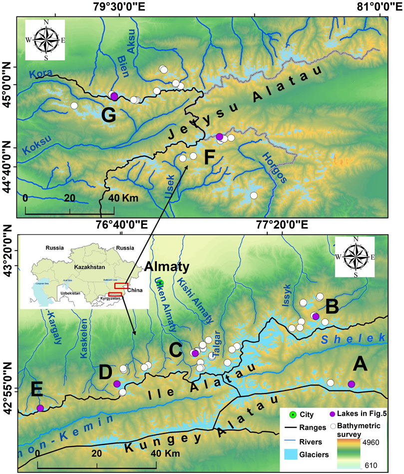
FIGURE 1. Study area. Letters indicate lakes shown in Figure 5.
This paper has three objectives. It presents and analyses bathymetric data from the conducted surveys and presents empirical relationships to reproduce lake geometry in the Tien Shan. It combines the survey data with the published bathymetric data compiling the largest global bathymetric data set for glacial lakes with natural dams to derive the scaling equations between depth/volume and area. In addition, the paper assesses the ability of GlabTOP2 to simulate lake bathymetry.
In the mountain ranges of the northern Tien Shan (Figure 1), glaciers occupied 565 km2 and 465 km2 in the Ile-Kungey (2008) and Jetysu Alatau (2011), respectively. Here, glaciers have been retreating since the 1950s losing about 0.8%–1% of their area per year (Severskiy et al., 2016). The abundance and area of proglacial lakes have been increasing in both regions (Bolch et al., 2011; Severskiy et al., 2013; Kapitsa et al., 2017; Kapitsa et al., 2018; Medeu et al., 2022). In the Jetysu Alatau, the abundance of lakes increased by 6% between 2000 and 2014 with the total count of proglacial lakes exceeding 600. Fifty lakes, whose potentail outburst can damage the existing infrastructure, were identified (Kapitsa et al., 2017). On the northern slope of the Ile Alatau, there were 154 proglacial lakes (Kapitsa et al., 2018) of which over 40 lakes were identified as dangerous (Bolch et al., 2011; Kapitsa et al., 2018). Characteristics of several dangerous lakes and GLOF events are discussed by Medeu et al. (2022). Since the beginning of the 20th Century, 55 GLOF events were registered across the study region. The frequency of GLOF peaked in the 1970s and 1980s (Kapitsa et al., 2017; Medeu et al., 2022) when strong positive temperature anomalies and enhanced snow and glacier melt were observed (Shahgedanova et al., 2018). An extensive lake management programme, implemented by the KSAMP, has resulted in the reduction of GLOF events. However, despite these efforts, seven GLOF occurred in the region in the 21st century causing damage to infrastructure. These events were caused by a combination of positive temperature anomalies, increase in runoff due to enhanced glacier melt in the headwater glacierized catchments, and enhanced melt of the subsurface ice. Further climatic warming is projected in the region and runoff is projected to stay high in summer in the extensively glacierized catchments under the more aggressive climatic scenarios sustaining glacial lakes (Shahgedanova et al., 2020).
Between 2009 and 2020, 74 bathymetric surveys were conducted on 57 lakes (Figure 1; Supplementary Table S1). Of these, 13 lakes are managed and bathymetries of 10 lakes were measured repeatedly following lake level lowering. All surveys were conducted in late July—August when lake levels are at their maximum. Using a classification of lakes given in Kapitsa et al. (2017), we identified most of the surveyed lakes either as glacier-connected lakes (Type 1; 21 lakes) or glacier-disconnected lakes positioned on the moraines formed in the 20th—21st centuries (Type 2; 28 lakes including Lake Kapkan). Lake Kapkan (Jetysu Alatau) changed from the Type 1 lake in 2011 to Type 2 lake in 2018 and was included in both categories. Eight lakes were positioned on the Little Ice Age (LIA) or older moraines (Type 3), and one was a rock-dammed lake (Type 4). There were no ice-dammed and supra-glacial lakes in the study region.
Lake depths were measured using Lowrancе LMS-480 echo sounder with a dual 200 kHz and 50 kHz frequency transducer and a GPS receiver enabling simultaneous soundings and position measurements. The 200 kHz frequency was used throughout all measurements because of the relatively small depths of the lakes. Heave was not accounted for because the small size of the lakes and calm weather on the days of surveys ensured that the surface of the water was still. The vertical uncertainty of Lowrancе LMS-480 200 kHz channel was ±0.1 m. The GPS receiver had a high estimated horizontal uncertainty of ±9 m and to improve the accuracy of the measurements, the simultaneous position measurements were taken using Garmin GPSMAP 64 with an estimated accuracy of ±3 m.
The echo sounder was rigidly attached to a float fasten to an inflatable boat (Figure 2A). Lake depths were measured over the entire area of the lakes along the bathymetry survey lines spaced at approximately 10–20 m with the along-profile increment of 3–10 m depending on the size of a lake. If the signal indicated sharp changes in depth, the density of measurements was increased. The mean density of measurements varied between three and 30 soundings per 1,000 m2 (Supplementary Table S1). In eight surveys (six lakes), the survey lines were spaced at about 50 m and these surveys can be identified in Supplementary Table S1 through the absence of the lake slope data (Figure 3 shows lake slope parameters).
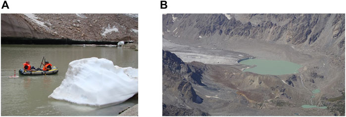
FIGURE 2. (A) Bathymetric survey of Lake No 9, Kishi Almaty basin, Ile Alatau and (B) Maksimov Lake, Shelek basin, Kungey Alatau.
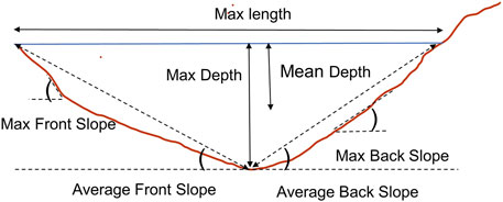
FIGURE 3. Diagram of the morphometric parameters of the surveyed lakes. Lake width (not shown) is measured along the lines perpendicular to the maximum length.
The obtained data were imported to ArcGIS. Two methods of interpolation—triangular irregular network (TIN) and Kriging—were applied to the point data, and compared. The difference between the outcomes was within the uncertainty of measurements estimated using standard error propagation formula applied to two terms: i) vertical uncertainty of depth measurements (±0.1 m) times lake area and Garmin GPSMAP 64 accuracy (±3 m). TIN was selected as a more computationally efficient method. Raster data sets were generated from TIN; and bathymetric maps with depth isolines were generated from the raster data sets. Morphometric parameters of the lakes were calculated using ArcGIS functions and used in the compilation of the bathymetric inventory.
The inventory of the surveyed lakes consists of i) geographical coordinates and altitude (defined as altitude of water surface at a time of the survey); ii) type of lake (including glacier-connected with glacier tongue); iii) morphometric parameters derived from the bathymetric surveys (Supplementary Table S1); iv) type of dam and drainage (partially completed and not included in this paper); iv) details of lake management, past GLOF, and presence of lakes upstream and downstream (lake cascades). The obtained morphometric parameters are illustrated by Figure 3. Maximum length (referred to as length) is defined as the longest straight line between two points on the waterline. It is not related to the orientation of a valley or position of an outlet because not all lakes have visible outlets. Maximum width (referred to as width) is the longest distance along the axis perpendicular to the length of the lake. Lake elongation was calculated as a ratio between lake’s width and length. Mean depth was derived from the three-dimensional raster data sets and volume values were calculated bathymetrically using ArcGIS. Following Muñoz et al. (2020) and in order to facilitate the compilation of the consistent regional data sets, we calculated maximum and average front slope (MaxFS, AFS) and maximum and average back slope (MaxBS, ABS) of the lakes (Figure 3). Back slope refers to the side next to (or in the direction of) glacier tongue and front slope refers to the opposite direction. In both cases, the average slope was measured from the top of the water level to the maximum depth (Figure 3).
In addition to the data derived from the surveys, lake areas were measured using satellite imagery from July-September 1999, 2001, 2007, 2008, 2017 and 2021 (Supplementary Table S2) using methodology described in Kapitsa et al. (2017), Kapitsa et al. (2018).
To avoid bias introduced by the repeated surveys, duplicate measurements were not used in the statistical analyses (except Figure 4 and Supplementary Figure S1 later in the text). Data from the latest surveys were used for those lakes which were surveyed multiple times (Supplementary Table S1). Values of mean lake depths and volumes were regressed against other morphometric parameters of the lakes. Two goodness-of-fit metrics were used to assess regression models: coefficient of determination (R2) and Mean Square Error (MSE). Following Huggel et al. (2004), relative error (RE) (defined as calculated minus measured value divided by calculated value) was used to compare measured and modelled depth and volume values. Standardized residuals (difference between measured and calculated values divided by standard deviation of the calculated value sample) were calculated and a standard threshold of ±2 was used to identify outliers. Statistical analyses were conducted using Minitab and R software.
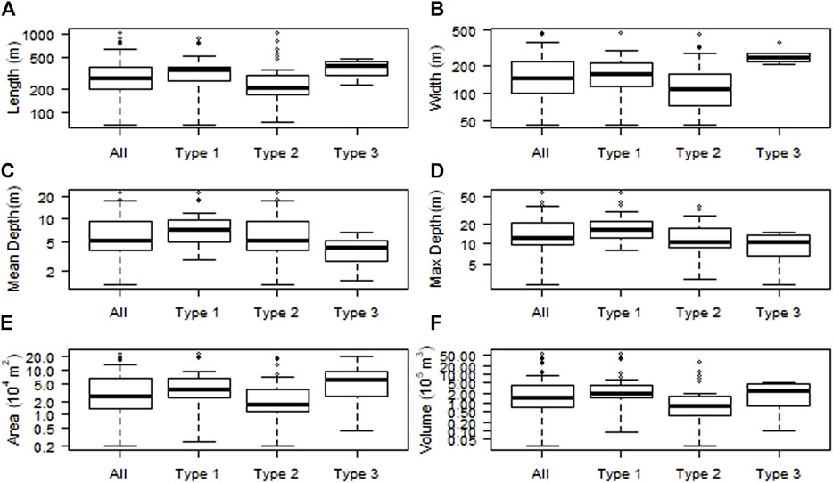
FIGURE 4. Boxplots for the selected parameters of the surveyed lakes including repeated surveys: (A) length; (B) width; (C) mean depth; (D) maximum depth; (E) area; (F) volume measured bathymetrically. Type 1—glacier-connected lakes, Type 2—lakes on the young moraines but without contact with glacier tongue, Type 3—lakes on the LIA or older moraines. Y-axes have a logarithmic scale.
Future hazard anticipation is becoming an important part of risk reduction. This approach relies on the prediction of future evolution of proglacial lakes. Here, we modelled the evolution of the existing glacier-connected Type 1 lakes using GlabTOP2 model which derives glacier bed topography based on glacier surface slope. GlabTOP2 is fully described in Frey et al. (2014) and its application to modelling the potential future lakes in the northern Tien Shan is discussed in Kapitsa et al. (2017). The model calculates ice thickness according to Eq. 1:
where h is ice thickness m), τ is basal shear stress, f is shape factor (0.8), ρ is ice density (900 kg m-3), g is acceleration due to gravity (9.81 m s-2) and α is glacier surface slope. The basal shear stress is estimated from an empirical relationship between τ and glacier height extent Δz (i.e., maximum elevation minus elevation of the glacier tongue) according to Haeberli and Hoelzle (1995).
We used glacier outlines as in 2000 obtained from regular cataloguing of glaciers of Kazakhstan (Severskiy et al., 2016) and the Shuttle Radar Topography Mission Digital Elevation Model (SRTM DEM) surface topography to model overdeepenings in which glacier lakes may form and expand. To reduce the influence of small-scale surface undulations in the ice thickness modelling, SRTM DEM with 30 m resolution was down-sampled to 45 m cell size which has been shown to generate the optimal results in GlabTOP2 modelling (Kapitsa et al., 2017). The overdeepenings in glacier beds were identified following the methodology outlined in Linsbauer et al. (2012); Linsbauer et al., 2016 and Kapitsa et al. (2017).
Glaciers have retreated since the baseline year of 2000 in the study region and Type 1 glacier-connected lakes have formed and expanded (Kapitsa et al., 2017; Kapitsa et al., 2018). The morphometric characteristics of the overdeepenings, corresponding to the Type 1 glacier-connected lakes formed in the predicted locations including area, volume, maximum and mean depth were derived and compared to the measured values. A comparison between the measured and modelled parameters is indicative because most lakes continue growing and a discrepancy between the modelled and the observed values can be due to both, the model error and uncertainty associated with the further growth of the lakes. However, the repeated surveys showed that mean lake depth is a conservative parameter which changed with time less than area (which mostly controls increase in volume) and we focused on assessing the ability of GlabTOP2 to simulate mean depth and bathymetry of the overdeepenings.
Table 1 and Figure 4 present the descriptive statistics of morphometric parameters of the surveyed lakes. The lake areas are relatively small ranging between 23.39x10⁴ (Maksimov Lake in the Kungey Alatau; Figure 2B; Figure 5A) to 0.2x10⁴ m2 but their median (2.87x10⁴ m2) and mean (5.55x10⁴ m2) areas are comparable with a mean area of 2.7x10⁴ m2 derived from a larger sample of over 600 lakes in the Jetysu Alatau (Kapitsa et al., 2017). The Type 1 (glacier-connected) lakes tend to have larger areas than the Type 2 lakes (forming on the young moraines) with the median areas of 5.75x10⁴ and 2.0x10⁴ m2, and mean areas of 6.85x10⁴ and 4.0x10⁴ m2, respectively. The Type 3 lakes (forming on the LIA moraines) had a mean area of 6.28x10⁴ m2. The sample include eight lakes only and their larger area is an artefact of focusing on larger lakes at risk of GLOF which are otherwise infrequent among the Type 3 lakes.
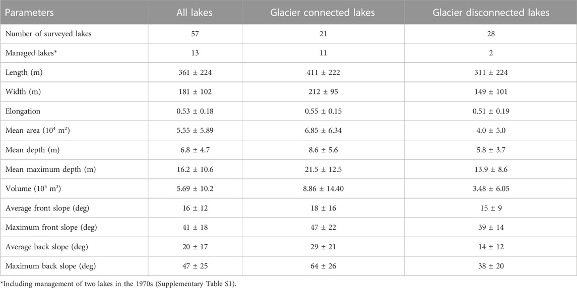
TABLE 1. Mean values ± standard deviations of the morphometric parameters of the surveyed glacier connected (Type 1) and glacier disconnected lakes young moraines (Type 2). In this and all other tables, repeated measurements are not included and data from the latest surveys are used for the repeatedly surveyed lakes. Lake Kapkan (Jetysu Alatau) changed from glacier connected in 2011 to glacier disconnected in 2018 and is counted in both categories except for the lake level lowering measures. Full range of values is shown in Figure 4.
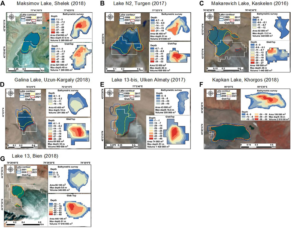
FIGURE 5. Measured and modelled bathymetries of the selected lakes. Numbers in parentheses refer to the years of bathymetric surveys. Locations of the lakes are shown in Figure 1 where they are indicated by the same letters as in this figure.
The surveyed lakes are relatively shallow. The median values of mean and maximum depths are higher for the Type 1 lakes at 8.3 and 19.0 m, respectively, against 4.6 and 10.5 m for the Type 2 and 3 lakes. The deepest lake in the sample is the glacier-connected Maksimov Lake which has the mean and maximum depths of 22.9 and 57.6 m, respectively (Figure 2B; Figure 5A). The deepest parts of the Type 1 glacier-connected lakes are usually those adjacent to the glacier tongues while in the Type 2 lakes, the middle parts of the lakes tend to be deeper. The average and maximum slope values for the surveyed sample are shown in Table 1. The median and mean values of ABS of Type 1 lakes are 18o and 29o against the respective AFS values of 13o and 18o while the median MaxBS value is 70o. For Type 2 lakes, the median and mean ABS values are 13o and 14o and the median value of the MaxBS is 32o. There is no significant difference between the AFS and MaxFS values of Type 1 and Type 2 lakes. Overall, the surveyed lakes have simple bathymetries due to their small size.
The largest median values of volume characterise the Type 3 lakes, which have larger areas and smaller depth, followed by Type 1 lakes which are deeper (Figure 4). The Maksimov Lake (Type 1 lake which is currently not managed) has the largest volume of 53.89x10⁵ m3.
Values of mean lake depths and volumes were regressed against other morphometric parameters of the lakes using data from the latest surveys. Regression against lake area, length, and width produced coefficients of determination significant at 5% confidence level (Supplementary Figure S1; Table 2). The relationships were stronger for the Type 1 lakes for which linear and polynomial relationships produced better results than the frequently used logarithmic and power fits with the R2 values of 0.76–0.78 and MSE of 7 m for the depth-area relationships (Table 2). For the Type 2 lakes, both lake area and width exhibited the strongest correlation with depth with R2 of 0.50–0.63 and MSE of 5–7 m (Table 2). The low MSE values are low implying small bias in the simulation of lake depths. For the whole sample, lake width and area were better predictors of depth than lake length but R2 values were lower than for the Type 1 group (Table 2) which has more homogenous characteristics (Figure 4). Other parameters did not correlate with depth either for the whole sample or for the Type 1 and Type 2 sub-samples. In particular, lake elongation, which has been used in other studies as a predictor of depth and volume (Qi et al., 2022), did not show significant correlation with either depth or volume in this data set.
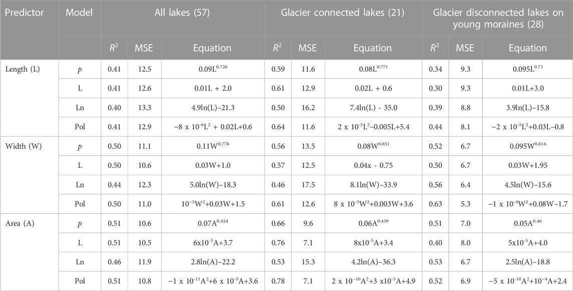
TABLE 2. Scaling equations linking mean depth and other morphometric parameters of the surveyed lakes for power p), linear L), logarithmic (Ln) and polynomial (Pol) models, coefficients of determination (R2), and Mean Standard Error (MSE; m) of regression. Results that are statistically significant at 0.05 confidence level are shown. Number of surveys in each sample is shown in parentheses.
Two lakes, Boskol and Lake N 4 in the Aksu catchment in the Jetysu Alatau (Supplementary Table S1) were identified as outliers in the regressions between mean depth and other morphometric parameters. Lake Boskol is a Type 3 lake formed on the LIA moraine. It has the third largest area of 19.75x10⁴ m2 but its depth does not exceed 7 m. Lake N 4 has usual shape with a length of 1,050 m (the largest in the data set), width of 230 m and elongation of 0.22.
While relationships between lake volumes and other morphometric parameters, especially area, are criticized for the inherent autocorrelation, they are useful in practical applications (Huggel et al., 2002; Wang et al., 2012; Loriaux and Casassa, 2013; Cook and Quincey, 2015; Khanal et al., 2015; Wood et al., 2021; Medeu et al., 2022). Results of regression between the bathymetrically derived volumes and other morphometric parameters are shown in Table 3. The highest coefficients of determination were obtained for the Type 1 glacier-connected lakes with R2 values ranging between 0.71 and 0.99. Lake area and mean depth were the best predictors. Regressing volume against mean depth achieved simultaneously the highest R2 and the lowest MSE values for the glacier-connected Type 1 lakes and for the whole sample. In general, power equations show the best fit but polynomial functions can be used to strengthen these further, e.g., between volume and area of Type 1 lakes where the use of polynomial function produces lower MSE value. There was substantial uncertainty in the estimation of volumes of larger lakes from depth and area when using power equations. Thus, volumes of the three largest lakes—Maksimov, Kapkan and Taskol with areas around 20x104 m2 and volumes in excess of 30x105 m3—were underestimated by 30%–40% (Figure 6A). The second-order polynomial equation provides a more accurate approximation of the volumes of Type 1 lakes including those of the larger lakes (Table 3; Figure 6A).
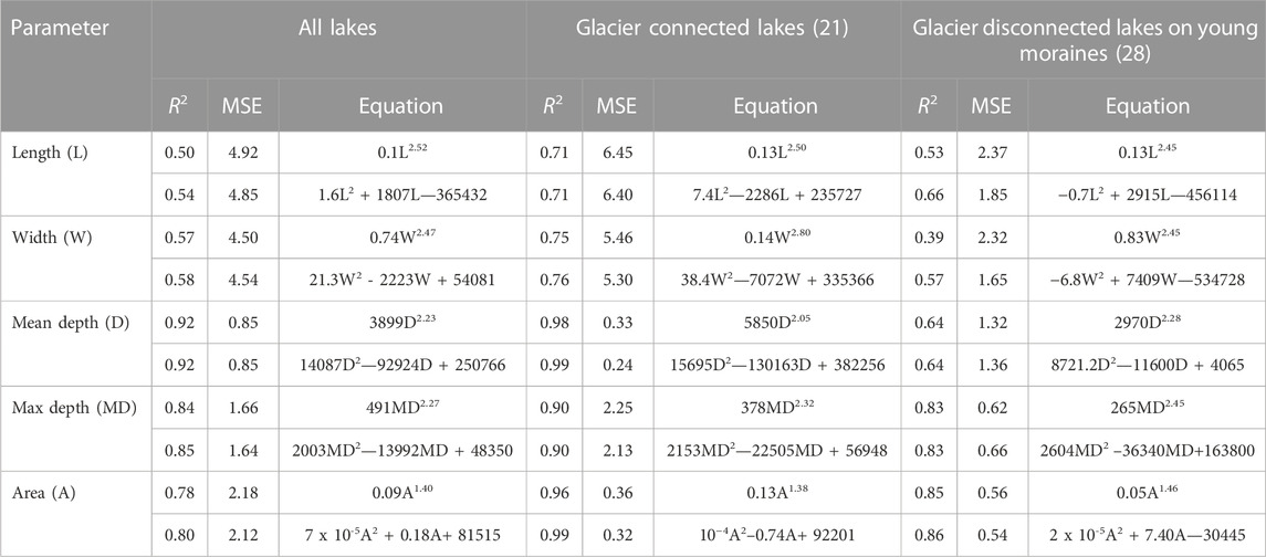
TABLE 3. Scaling equations, coefficients of determination (R2), and Mean Square Error (MSE, 1011 m3) between the bathymetrically derived lake volume and other morphometric parameters of the surveyed lakes. Results are statistically significant at 0.05 confidence level.
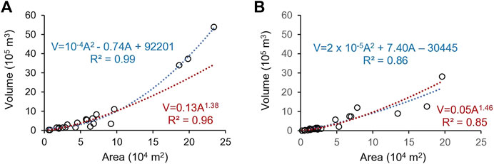
FIGURE 6. Power (red) and polynomial (blue) area (A)—volume (V) relationships for (A) glacier-connected lakes and (B) glacier-disconnected lakes on young moraines.
The ability of the morphometric parameters to predict volume was lower for the Type 2 lakes and the combined data set containing all lakes. Using area as predictor allowed maximizing R2 and minimizing MSE for the Type 2 lakes. In addition to area, maximum depth and lake width were the two parameters which predicted volume of Type 2 lakes best. There was no difference between the performance of the polynomial and power equations (Figure 6B).
The obtained power equations linking mean depth and area (Table 2) and volume and area (Table 3) were tested using the independent data sets of lake depths and bathymetrically derived volumes compiled by Huggel et al. (2002), Wang et al. (2013), Cook and Quincey (2015), Zhang et al. (2023) and the original data by Janský et al. (2010), Muñoz et al. (2020), and Zhang et al. (2023). Duplicate measurements were excluded from all data sets. Data for volumes only were used from Zhang et al. (2023) because maximum instead of mean depth was reported in this study. Two lakes [Leones in Patagonia (Harrison et al. (2008); Loriaux and Casassa (2013)] and Galong Co [China (Zhang et al., 2023)] were excluded from the assessment of volume calculations because their volumes are an order of magnitude higher than those of any other lake in the sample (Supplementary Table S3). Data for the lakes with natural dams only were used from Muñoz et al. (2020). The compiled data includes three types of lakes (Table 4), two of which—ice-dammed and supra-glacial—did not occur in our study area. We could not verify the accuracy of the published measurements excluding only the data for the Brazo Rico Lake in South Patagonia from the Cook and Quincey (2015) data set because depth measurements were provided for the lake areas adjacent to the glacier tongue instead of the mean depth (Stuefer et al. 1999; Stuefer et al., 2007) and were a clear outlier. The combined samples contained 159 and 188 lakes for the assesment of depth and volume calculations, respectively (Supplementary Table S3). On average, lakes in the published data sets were larger than in our bathymetrical data set with means and standard deviations of (5.91 ± 10.26)x105 against (5.6 ± 5.9)x104 m2 for areas and 21.6 ± 23.1 and 6.8 ± 4.7 m for depth, respectively.
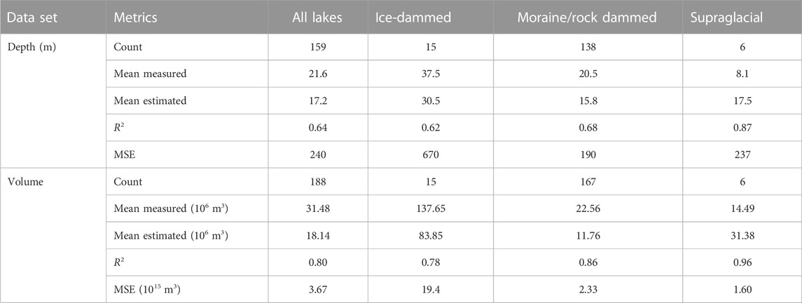
TABLE 4. Comparison between the measured and calculated lake depths and volumes. The power equations for the Type 1 lakes were used (Table 2; Table 3). Measured data are from Huggel et al. (2002), Janský et al. (2010), Wang et al. (2013), Cooke and Quincey (2015), Muñoz et al. (2020), and Zhang et al. (2023).
Table 4 shows the results of the application of the power area-depth and area-volume equations for the Type 1 glacier-connected lakes (Tables 2 and 3) which showed marginally better performance than the equations for the Type 2 glcier disconnected and all surveyed lakes. There was a close correlation between the modelled and measured depths of the moraine, rock and ice-dammed lakes with the R2 value of 0.62—0.68 with and R2 value of 0.64 for all lakes (Figure 7A). On average, the modelled values were 5–7 m lower than the measured values. The errors of the regression models, however, were higher with the lowest MSE value of 190 m obtained for the moraine and rock-dammed lakes. A high MSE value of 670 m obtained for the ice-dammed lakes results from a large error in the calculation of mean depth of Lake No Lake (155 m against the calculated value of 56 m). Removal of this lake from the assessment reduces MSE for the ice-dammed lakes to 80 m. By contrast, depth of the supraglacial lakes was overestimated. Correlation between the measured and modelled depths of the supraglacial lakes was strong (R2 of 0.87) but it was derived from a very small sample.
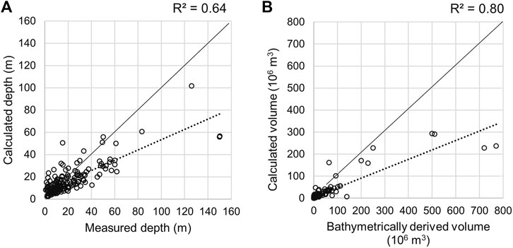
FIGURE 7. Calculated versus (A) measured depth and (B) bathymetrically derived volume. Straight dashed and solid lines are regression and X=Y lines, respectively.
RE were calculated to assess the ability of the new equations to predict depths and volumes of individual lakes. The lakes were binned into four categories according to the assigned RE (Table 5). Cook and Quincey (2005) characterised lakes whose depth was calculated with an error of over ±49% as “unpredictable”. A large discrepancy, however, can reflect systematic bias. In this study, standardized residuals exceeding a threshold of ±2 were used to identify outliers.
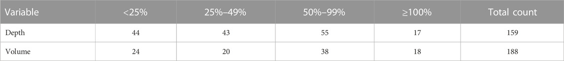
TABLE 5. Count of lakes in four relative error (RE) categories. Absolute values of RE are used.
Overall, depths of 55% of all lakes were calculated with an error less than ±49% (Table 5). The standardized residuals were generally higher for lakes with depth greater than 20 m but the critical threshold was exceeded for seven lakes only. The highest underestimation characterised two large lakes—Nef in North Patagonia (Loriaux and Casassa, 2013) and Lake No Lake in British Columbia (Geertsema and Clague, 2005)—with areas greater than 50x105 m2 and depth of 150 m. Both lakes are deep for their surface areas. Other formulae were applied to and failed to predict the depth of Lake No Lake (Cook and Quincey, 2015). On average, the lowest error (±34%) was obtained for the ice-dammed lakes exceeding 49% only for Lake No Lake. The sample of ice-dammed lakes is relatively small (Table 4) which makes its sensitive to outliers. If Lake No Lake is removed from the sample, R2 between the measured and modelled depths of the ice-dammed lakes increases to 0.84 and RMSE changes from ±25.9 m to ±9.3 m. Predictability of the moraine- and rock-dammed lake depth varied strongly within the sample. In addition to Lake Nef, depths of lakes Maud in New Zealand (Allen et al., 2009) and Auquiscocha, Purhuay, and Rusgo in the Andes (Muñoz et al., 2020), exceeding 40 m, were strongly underestimated. However, correlation between the measured and modelled depths was stable and not significantly affected by the removal of the outliers. Among the supraglacial lakes, a shallow Lake Petrov in the Tien Shan is an outlier whose depth was not reliably predicted by the previously published scaling equations (Cook and Quincey, 2015). The lake is positioned on a debris-covered glacier terminus and experiences strong seasonal fluctuations in area and depth (Janský et al., 2010).
There was a strong correlation between the calculated and bathymetrically measured volumes of lakes with R2 value of 0.80 for the overall sample (Table 4; Figure 7B). Volumes were calculated with an error of less than ±49% for 44% of the lakes (Table 5). Derived from a sample of smaller lakes, the scaling equation generally underestimated volumes except for the supraglacial lakes whose volumes were overestimated (Table 4). Results for the ice-dammed lakes were affected by the inclusion Lake No Lake in the sample and improve significantly if this outlier is removed with R2 value increasing to 0.94 and a smaller difference between measured and calculated values which became 96.05x10⁶ and 73.53x10⁶ m3, respectively. In addition to Lake No Lake, four other large lakes—Nef (770.7x10⁶ m3) in Patagonia (Loriaux and Casassa, 2013), Tasman (510.0x10⁶ m3) in New Zealand (Robertson et al., 2012), Phantom (500.0x10⁶ m3) in Axel Heiberg Island (Maag, 1963), and Rewoco (139.0x10⁶ m3) in China (Zhang et al., 2023)—were identified as outliers (with standardized residuals exceeding the threshold of ±2) whose volumes were significantly underestimated (Figure 7B). The Petrov Lake in the Tien Shan Janský et al. (2009) was an outlier whose volume was overestimated by 61%.
To expand the samples of measured depths and bathymetrically derived volumes of large lakes and those types of lakes which do not occur in the study area, we combined the newly obtained and published data. The measured depth and bathymetrically derived volume data sets included data for 216 and 245 lakes with natural dams excluding duplicate measurements (Figure 8A; Supplementary Table S3). There is a good correlation between lake depth and area with R2 values of 0.67 overall and 0.71 for the moraine- and/or rock-dammed lakes. This is comparable with the results obtained in this study for the more homogeneous group of smaller glacier-connected lakes (Table 2) and a significant improvement on the results by Cook and Quincey (2015) who reported stronger variability in lake depth for any given area with R2 of 0.38 derived from a smaller data set of 42 lakes. Analysis of standardized residuals shows that three lakes remain outliers in the combined depth data set (Figure 8A) and their removal from the data set reduces MSE by half. The values of standardized residuals are higher for the lakes with depths of 20–60 m than for lakes with depths of under 20 m.
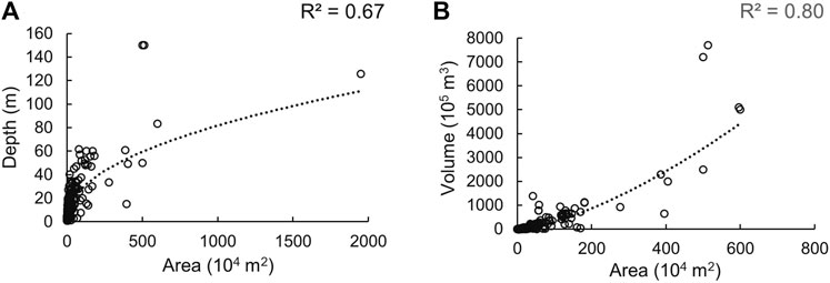
FIGURE 8. Regression between lake area and (A) depth and (B) bathymetrically derived volume for the combined data set.
The obtained bathymetries provided a unique opportunity to evaluate the skill of GlabTOP2 in simulating bathymetries of 18 Type 1 glacier-connected lakes. The measured lake areas and volumes in this sample varied between 0.79x10⁴ and 23.39x10⁴ m2 and between 0.22x10⁵ and 53.89x10⁵ m3, respectively. The modelled and measured mean depth values (±standard deviation) were 13.1 ± 5.9 and 9.3 ± 5.6 m, respectively. The mean maximum depth values were 32.5 ± 15.3 and 21.3 ± 12.5 m, respectively. Lake 13 in the Bien catchment is an outlier (discussed further in the text) and excluded from this comparison.
Figure 5 further illustrates the observed and predicted evolution of the selected lakes identified as dangerous (Kapitsa et al., 2018; Medeu et al., 2022). There is a good agreement between the modelled and measured bathymetries of the Maksimov Lake (Figure 5A). The measured and modelled maximum and mean depths values were 58 and 22 m against 50 and 20 m, respectively. The lake’s area and volume are projected to reach an of 45.45x10⁴ m2 and 107.39x10⁵ m3, respectively, and a small slope of the glacier tongue (Figure 2B) indicates that the lake will indeed continue growing. A single bathymetric survey of the lake was conducted in 2018 and there is no information about actual changes in its depth. The multiple measurements of its area using satellite data showed that it doubled between 1999 and 2021 although the rate of area growth slowed down from 5% per year in 1999–2007 to 2.5% per year in 2017–2021 (Figure 5A). This comparison provides confidence in and raises concerns about the predicted growth of the lake which is projected to remain the largest in the Ile-Kungey Alatau. Although the lake’s dam is composed mostly of solid rock reducing the risk of GLOF, the lake is partially contained by a moraine dam (Figure 2B). Seismic activity, common in the region, may affect the rock dam too raising level of the potential hazard which is predetermined by lake volume and maximum peak discharge controlled by volume (Emmer and Vilímek, 2013).
There is a close agreement between the modelled and measured depth of Lake N 2 in the Turgen basin (Figure 5B). Its area increased from 2.25x10⁴ to 8.05x10⁴ m2 between 1999 and 2021, however, GlabTOP2 does not predict any further increase. The Makarevich Lake in the Kaskelen basin is increasing in line with the GlabTOP2 results although the modelled depth in the sector of the lake adjacent to the glacier exceeds the measured values (Figure 5C). While the model error is not excluded, the regular drainage of the lake via the artificial channels may contribute to this discrepancy. Repeated surveys of the Galina Lake in the Uzun-Kargaly basin are required to establish whether the lake’s depth, currently reaching 19 m, is likely to reach the projected depth in excess of 30 m (Figure 5D).
Lake 13-bis in the Ulken Almaty catchment was identified one of the most dangerous lakes in the Ile Alatau (Kapitsa et al., 2018; Medeu et al., 2022). Its area and volumes increased from 3.05x10⁴ to 4.3x10⁴ m2 and 1.8x10⁵ to 3.05x10⁵ m3, respectively, between 2011 and 2015 but declined afterwards due to the implementation of artificial lake drainage. Its mean and maximum depths reached 7 and 17 m, respectively, before 2015. These values are consistent with the GlabTOP2 predictions for the same sector of the lake (Figure 5E). Further increase in the lake’s area and depth are projected and further bathymetric surveys are required to establish if the lake is likely to reach the projected depths. By contrast, no further increase is projected for one of the most dangerous and the second largest in the data set Lake Kapkan (37.25x10⁵ m3) in the Jetysu Alatau (Kapitsa et al., 2017). Observations confirmed that the lake changed from Type 1 in 2011 to Type 2 in 2018 (Figure 5F) and there is no further potential for increase in lake area and volume.
Overall, GlabTOP2 simulates realistic depth values although there is a tendency towards the overestimation in comparison with the measured depths. In the assessed data set, there was a single outlier—Lake 13 in the Bien River catchment, Jetysu Alatau—where the parameters of the modelled overdeepening substantially exceeded the measured parameters (Figure 5G). The projected maximum and mean depth were 80 and 39 m, respectively. The maximum and mean lake depths measured in 2018, were 10 and 5 m in the sector of the lake where the largest depths were modelled. Importantly, the whole overdeepening, which now contains two lakes (Figure 5G), does not reach the depth and volume projected by the model.
Information about volumes of glacier lakes is important for modelling GLOF and runout distances of the floods. However, there are few direct measurements of lake depth and volumes which can only be obtained through bathymetric surveys. The current data set, derived from 74 surveys of 57 lakes, significantly improves data availability. It enables detailed characterization of lake bathymetries improving risk assessments by the regional risk-reduction agency KSMP in the Tien Shan where GLOF events cause substantial damage to the downstream communities and ecosystems (Medeu et al., 2022). It also enables better understanding of statistical relationships between morphometric parameters of glacial lakes in the region. It helps to establish more robust empirical relationships between area, depth and volume of glacial lakes globally when combined with the previously published data.
Area-depth and area-volume relationships, developed from the regional and global data sets, were widely applied in Central Asia (Konovalov, 2009; Konovalov and Rudakov, 2016; Medeu et al., 2022). Table 7 and Supplementary Figure S2 show a comparison between the bathymetrically derived values of lake volumes and depths and values calculated from the lake areas using equations published in the literature and derived in this study. Most equations produced similar R2 values. There was a closer correlation between the estimated and measured values of lake volumes (R2 values of 0.78–0.97) while there were larger discrepancies between the calculated and measured depths (R2 values of 0.50–0.68). For both parameters, there was a closer agreement with the measured parameters of the Type 1 glacier-connected lakes. The mean absolute values of RE were mostly moderate ranging between 25% and 40% and were lower for the Type 1 lake depth (Table 7). Higher errors in the calculation of volumes of the glacier-connected lakes resulted from the formula derived by Wang et al. (2012) based on the published surveys of the moraine-dammed lakes in the Himalayas. The application of the formula proposed by Fujita et al. (2013) for the calculation of lake depth in the Himalayas resulted in a strong overestimation of lake depths probably because it was derived from a sample of much larger lakes.
The area-depth relationships by Huggel et al. (2002), Wang et al. (2012) and the power equation for Type 1 lakes derived in this study produced the lowest mean absolute RE of 26% for lake depth. The formula by Khanal et al. (2015) produced the lowest mean absolute RE in the estimation of lake volumes with the formulae by Cook and Quincy (2015), Huggel (2002) and the one derived in this study producing similar results. Analysis of the actual RE values showed that most formulae overestimated depth and volume of smaller lakes with mean depths less than approximately 15 m (Supplementary Figure S2) generating positive bias in the calculated values (Table 7). The newly developed scaling equations do not have this limitation as errors of the depth and volume regression models are randomly distributed while the use of polynomial functions helps to avoid underestimation of depths and volumes of larger lakes. We note, however, that equation developed by Evans (1986) also produced randomly distributed errors and no systematic bias in the calculated depths and volumes of lakes with depths under 15 m (Supplementary Figure S2) while the equation by Popov (1991) produced randomly distributed errors for volumes of the shallow lakes.
All power functions underestimated depths and volumes of the lakes with mean depths and volumes exceeding 15 m and 3x10⁶ m3, respectively. (Supplementary Figure S2). The formula by Popov (1991) produced the largest errors underestimating volumes of larger lakes by 38%–82%. The use of the second-order polynomial function reduced the error of simulating volumes of larger lakes to 0%–4% and is recommended for a more accurate approximation of depths and volumes of the larger glacier-contact lakes in the study region.
In the global context, the main contribution is in a significant increase of the available bathymetries of glacial lakes. This helps constrain uncertainty of the application of area-depth and area-volume equations to the large and non-homogenous data sets and enables researchers to devlop sub-samples of lake depths and volumes to derive scaling equations for lakes of different types and sizes. The power equations derived from the combined data set of over 260 lakes (Supplementary Table S3) had the R2 values of 0.67–0.71 and 0.80–0.85 for depth and volume, respectively (Table 6). This is a considerable improvement on the results derived by Cook and Quincey (2015) from a smaller global data set. However, uncertainty in simulating lake depths and volumes using the combined data set increases with lakes’ size. While the values of standardized residuals do not exceed ±1 for the lakes with depth below approximately 20 m, there is a notable trend for higher residuals for lakes deeper than 20—30 m. Therefore, more measurements of larger lakes, which tend to be deeper, are needed. Supraglacial lakes form a distinct sub-sample of lakes whose depths are consistently underestimated by the developed equations (Table 4). This limitation was also noted by Cook and Quincey (2015). There is a limited number of surveys of supraglacial lakes globally (Table 4, Supplementary Table S3) and wider data acquisition is required.
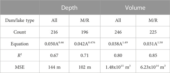
TABLE 6. Scaling equations for mean depth (D; m) and volume (V; m3) based on lake area (A; m2) derived from the data sets combining published data and data obtained in this study (Supplementary Tables S1, S3). M/R is moraine- and rock-dammed lakes. Repeated measurements are not included and data from the latest surveys are used for the repeatedly surveyed lakes.
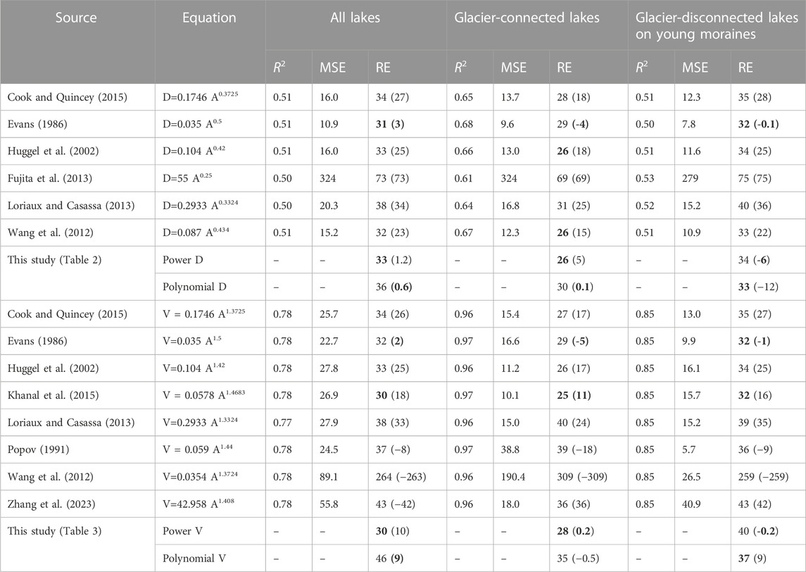
TABLE 7. Coefficients of determination (R2), MSE, and RE (%) between the measured and estimated lake volumes and depths. V is volume (m3), D is depth m) and A is area (m2 except Fujita et al. (2013); Zhang et al. (2023), where area is in km2). MSE for volume is in 1010 m3. Absolute values of RE are shown with mean actual RE values given in parentheses. Equations derived in this study for all lakes, Type 1 and Type 2 lakes are shown in Tables 2 and Table 3. The lowest RE values resulting from the published and derived equations are shown in bold.
The results of the bathymetric and remote sensing surveys are used by practitioners (KSAMP) in conjunctions with the GlabTOP2 projections (Kapitsa et al., 2017; Kapitsa et al., 2018) to improve efficiency of lake monitoring and management by focusing on those lakes which are reliably predicted to grow in the future in addition to those posing immediate risk. Lake management involves lowering lake levels by installing syphons and construction of the artificial drainage channels. This practice proved efficient in the prevention of GLOF whose frequency peaked in the 1970s when strong positive temperature anomalies and glacier melt were observed in the region (Shahgedanova et al., 2018). In 1971–1980, 20 GLOF occurred while a single lake was managed. By contrast, there were four GLOF since 2001 despite the observed climatic warming and accelerating glacier retreat because KSMP significantly increased the number of managed lakes to 26 (Supplementary Figure S3) reducing risk of GLOF which was otherwise identified as high on the global scale (Taylor et al., 2023). However, lake level lowering measures are expensive and require the deployment of extensive workforce and machinery in the challenging mountain environments (Medeu et al., 2022). Bathymetric surveys and modelling of lake expansion are important tools enabling decision-makers to optimize the risk reduction measures.
The repeated bathymetric surveys of Lake Kapkan (37.25x10⁵ m3) in the Jetysu Alatau, which is the second largest in the data set and one of the most dangerous in the region (Kapitsa et al., 2017), showed that its mean and maximum depths were reduced from 19 to 41 m, respectively, in 2011 to 14 and 36 m in 2018 following the artificial lake drainage. A significant reduction in the volumes of the extremely dangerous lake 13-bis in the Ulken Almaty catchment and Lake Manshuk in the Kishi Almaty catchment have been achieved since 2015 (Supplementary Table S1). Monitoring of Maksimov Lake was initiated on the basis of the GlabTOP2 modelling output which predicted a strong growth of the lake (Kapitsa et al., 2018) while the projected growth of Makarevich Lake provided justification for funding of the lake level lowering measures. The KSAMP aims to implement risk avoidance measures in addition to risk reduction by advising regional authorities and planning agencies on future dangers of lake formation in specified locations. This approach has become a part of the regional strategy of adaptation to climate change. It is, therefore, important that the model outputs are validated.
The comparison of measured and modelled bathymetries is indicative because most lakes continue growing and it is not possible to use any quantitative metrics. The inspection of the measured and modelled bathymetries of the Type 1 glacier-connected lakes (Figure 5) showed that most simulations provided realistic results although it appears that GlabTOP2 tends to overestimate lake depth. In the case of Lake 13 in the Bien catchment (Figure 5G), ClabTOP2 failed to reproduce the measured parameters of the overdeepening containing the lake. We attribute it to the significant overestimation of ice thickness: the simulated maximum depth was 168 m against the typical measured values of 30–60 m (Cherkasov, 2004).
We attempted to assess uncertainty by comparing the modelled ice thickness with ice thickness values compiled by Farinotti et al. (2019) from four different models: Huss and Farinotti (2012), Frey et al. (2014) (who used GlabTOP2 but with settings different to the ones applied in this study), Maussion et al. (2019), and Fürst et al. (2017). The values of maximum ice depth and its standard deviation were derived for each glacier terminating in the lake for which overdeepenings were modelled and measured bathymetric data were available. Overdeepenings were derived from each of the four models’ ice thickness data sets and their bathymetries were compared with our simulations using GlabTOP2 and with measured bathymetries (Supplementary Table S4). Overall, 15 glaciers and lakes were used in this comparison because data in the Farinotti et al. (2019) data set were not available for all glaciers. In case of managed lakes, we used bathymetries obtained before lake level lowering commenced.
This comparison has several limitations. Firstly, in our study, glacier outlines from 2000 (or nearby year) were used as contemporaneous with the SRTM data acquisition. The published ice thickness values were based on the glacier outlines from the Randolph Glacier Inventory (RGI) 6.0 (RGI Consortium, 2017) obtained in later years. This difference affects modelled bathymetries of the overdeepenings under the rapid glacier retreat in the study region. For example, one of the most dangerous Lake 13-bis in the Ulken Almaty catchment began to form in 2000 while by 2015, its volume had reached 4.3x10⁵ m3 and lake lowering measures commenced (Supplementary Table S2). Therefore, our simulation generates a larger area of its overdeepening than the simulations based on the later glacier outlines. Secondly, the assessed sample of lakes was small while the between-model variability was high (Supplementary Table S4).
Despite the limitations, the comparison of different ice thickness simulations highlighted indicators of errors in modelling overdeepenings using GlabTOP2. The mean values and standard deviations of ice thickness of the selected 15 glaciers were 73 ± 15 m in our study and 96 ± 19, 75 ± 16, 84 ± 20, and 61 ± 14 for models one to four, respectively. A strong between-model discrepancy in the simulated ice thickness was observed in a number of cases and was indicative of error in modelling overdeepenings. In case of Lake Bien, the maximum ice thickness of the adjacent glacier varied between 164 m (Huss and Farinotti, 2012), which is close to the value obtained in this study, and 99 m (Fürst et al., 2017) and all models appeared to have overestimated ice thickness (Cherkasov, 2004). In case of Maksimov Lake, which was simulated accurately using the GlabTOP2 data (both, from this study and from model 2 (Frey et al., 2014)), there was a closer agreement between all models in simulation of the maximum ice thickness with values ranging between 100 m (Fürst et al., 2017) and 130 m (Frey et al., 2014). Closer examination of the simulated ice thickness showed that overestimation occurred where glaciers change directions of their flow. These two criteria can be used in the future in the assessment of uncertainty.
Of all assessed models, GlabTOP2, as used in this study and by Frey et al. (2014), provided realistic simulations of overdeepening bathymetries (Supplementary Table S4; Supplementary Figures S4–S6). Results based on ice thickness from Frey et al. (2014) underestimate lake depth predicting the mean depth of future overdeepenings as 7.0 m against the currently observed value of 8.4 m (Supplementary Figure S4). For example, the Maksimov Lake was predicted to achieve mean depth of 12.6 m against the currently observed 22.9 m (Supplementary Figure S5). Other three models significantly underestimated area, volume, and depth (with average values of future mean depth of 2.0—3.6 m) and are not recommended for the simulation of overdeepenings in the study area. We note, however, that model 1 (Huss and Farinotti, 2012) provided a more realistic representation of bathymetry of Lake Bien 13 (Figure 7G) which was overestimated by both GlabTOP2 simulations (Supplementary Figure S6).
This paper presented a new bathymetric data set from the northern Tien Shan considerably improving the availability of glacial lake bathymetric data globally. The depth and volume scaling relationships for glacial lakes of different types were derived from the conducted bathymetric surveys and from a combined global data set of over 260 lakes including the published bathymetric data. The compiled inventories and scaling equations are designed to help practitioners assess the potential impacts of GLOF.
The main conclusions are as follows.
(i) There are statistically significant relationships between lake depth and area, length, and width in the study area. The obtained coefficients of determination were moderate to high (0.56–0.78) and MSE and RE values moderate to low. The provided assessment of a range of scaling equations derived from our surveys and published in the literature showed that their performances varied between different types of lakes. This should help researchers and practitioners make an informed choice;
(ii) As in many other studies, there is a strong correlation between area and bathymetrically derived volume particularly for the glacier-connected lakes. However, relative errors are high for many lakes. The power equations significantly underestimate depths and volumes of larger lakes. Polynomial model provided a closer fit and is recommended for the simulation of volumes of larger lakes in the study region;
(iii) Global data sets of measured lake depths and bathymetrically-derived volumes have been compiled using data published in the literature and derived from this study. Scaling relationships between lake depth and area have been improved showing higher coefficients of determination in comparison with previous studies based on the smaller samples;
(iv) There were two distinct groups of lakes whose simulated depths and volumes exhibited higher uncertainty: larger lakes with mean depth in excess of 20 m and shallow supraglacial lakes. To reduce uncertainties in the derived scaling equations, future surveys should focus on lakes of these types;
(v) Lake bathymetries, simulated by GlabTOP2, are mostly in agreement with the measured bathymetries. Although the model, as used in our study tends to overestimate lake depth, comparison with the published data suggests that it can be further calibrated to improve its accuracy. This conclusion confirms that the model is a useful adaptation tool which can be applied by the practitioners to reduce and avoid risks of GLOF.
The original contributions presented in the study are included in the article/Supplementary Material, further inquiries can be directed to the corresponding author.
VK, MS, and IS designed the study; VK, NK, MK, and AY conducted the surveys; VK, MS, NK, and MT processed and analysed the data; MS wrote the original manuscript. All authors contributed to the article and approved the submitted version.
UK Newton—al Farabi Fund, “Climate Change, Water Resources and Food Security in Kazakhstan” grant number 172722855; UK Global Challenges Research Fund, “Central Asian Research and Adaptation Water Network (CARAWAN),” grant number GCRFNGR3\1389; University of Reading (UK) Building Outstanding Impact Support Programme (BOISP) “Assessment of risks of glacier lake outbursts using remote sensing and glacier bed topography (GlabTop) modelling in the Tien Shan, Central Asia”; Kazakhstan Programme of Targeted Financing of Scientific Research, “Glacial Systems of the Transboundary Basins of Central Asia: Current State, Observed and Projected Changes, and Role in the Provision of Water Security in the Region,” grant number BR18574176; UKRI Rapid Response Policy Engagement Fund “Bridging over troubled waters: Improving preparedness and reducing vulnerability to debris flow in Central Asia.”
The authors are grateful to the Kazakhstan State Mudflow Protection Agency (KSAMP) for the provision of helicopter flights and colleagues from the Kazakhstan Institute of Geography for their assistance with the field surveys.
The authors declare that the research was conducted in the absence of any commercial or financial relationships that could be construed as a potential conflict of interest.
All claims expressed in this article are solely those of the authors and do not necessarily represent those of their affiliated organizations, or those of the publisher, the editors and the reviewers. Any product that may be evaluated in this article, or claim that may be made by its manufacturer, is not guaranteed or endorsed by the publisher.
The Supplementary Material for this article can be found online at: https://www.frontiersin.org/articles/10.3389/feart.2023.1192719/full#supplementary-material
Allen, S. K., Schneider, D., and Owens, I. F. (2009). First approaches towards modelling glacial hazards in the Mount Cook region of New Zealand’s Southern Alps. Nat. Hazards Earth Syst. Sci. 9, 481–499. doi:10.5194/nhess-9-481-2009
Bolch, T., Peters, J., Yegorov, A., Pradhan, B., Buchroithner, M., and Blagoveshchensky, V. (2011). Identification of potentially dangerous glacial lakes in the northern Tien Shan. Nat. Hazards 59 (3), 1691–1714. doi:10.1007/s11069-011-9860-2
Carrivick, J. L., and Tweed, F. S. (2013). Proglacial Lakes: character, behaviour and geological importance. Quat. Sci. Rev. 78, 34–52. doi:10.1016/j.quascirev.2013.07.028
Cherkasov, P. A. (2004). Raschet sostavlyaushih vodno-lednikovogo balansa vnutrikontinentaloj lednikovoj sistemy (quantifying components of water and glacier balances of a continental glacier system). Almaty, Kazakhstan: Kaganat Publishers, 334. In Russian.
Colonia, D., Torres, J., Haeberli, W., Schauwecker, S., Braendle, E., Giraldez, C., et al. (2017). Compiling an inventory of glacier-bed overdeepenings and potential new lakes in de-glaciating areas of the Peruvian Andes: approach, first results, and perspectives for adaptation to climate change. WaterSwitzerl. 9 (5), 336. doi:10.3390/w9050336
Cook, S. J., Kougkoulos, I., Edwards, L. A., Dortch, J., and Hoffmann, D. (2016). Glacier change and glacial lake outburst flood risk in the Bolivian Andes. Cryosph 10, 2399–2413. doi:10.5194/tc-10-2399-2016
Cook, S. J., and Quincey, D. J. (2015). Estimating the volume of Alpine glacial lakes. Earth Surf. Dyn. 3 (4), 559–575. doi:10.5194/esurf-3-559-2015
Emmer, A., Allen, S. K., Carey, M., Frey, H., Huggel, C., Korup, O., et al. (2022). Progress and challenges in glacial lake outburst flood research (2017–2021): A research community perspective. Nat. Hazards Earth Syst. Sci. 22, 3041–3061. doi:10.5194/nhess-22-3041-2022
Emmer, A., and Vilímek, V. (2013). Review article: lake and breach hazard assessment for moraine-dammed lakes: an example from the cordillera blanca (Peru). Nat. Hazards Earth Syst. Sci. 13 (6), 1551–1565. doi:10.5194/nhess-13-1551-2013
Evans, S. G. (1986). “Landslide damming in the cordillera of Western Canada,” in Landslide dams: Processes, risk, and mitigation. Editor R. L. Schuster (American Society of Civil Engineers, Geotechnical Special Publication), 3, 111–130.
Farinotti, D., Huss, M., Fürst, J. J., Landmann, J., Machguth, H., Maussion, F., et al. (2019). A consensus estimate for the ice thickness distribution of all glaciers on Earth. Nat. Geosci. 12, 168–173. doi:10.1038/s41561-019-0300-3
Frey, H., Machguth, H., Huss, M., Huggel, C., Bajracharya, S., Bolch, T., et al. (2014). Estimating the volume of glaciers in the Himalayan–Karakoram region using different methods. Cryosph 8, 2313–2333. doi:10.5194/tc-8-2313-2014
Fujita, K., Sakai, A., Takenaka, S., Nuimura, T., Surazakov, A. B., Sawagaki, T., et al. (2013). Potential flood volume of Himalayan glacial lakes. Nat. Hazards Earth Syst. Sci. 13 (7), 1827–1839. doi:10.5194/nhess-13-1827-2013
Furian, W., Loibl, D., and Schneider, C. (2021). Future glacial lakes in High Mountain Asia: an inventory and assessment of hazard potential from surrounding slopes. J. Glaciol. 67 (264), 653–670. doi:10.1017/jog.2021.18
Fürst, J. J., Gillet-Chaulet, F., Benham, T. J., Dowdeswell, J. A., Grabiec, M., Navarro, F., et al. (2017). Application of a two-step approach for mapping ice thickness to various glacier types on Svalbard. Cryosphere 11, 2003–2032. doi:10.5194/tc-11-2003-2017
Gardelle, J., Arnaud, Y., and Berthier, E. (2011). Contrasted evolution of glacial lakes along the Hindu Kush Himalaya mountain range between 1990 and 2009. Glob. Planet. Change 75 (1–2), 47–55. doi:10.1016/j.gloplacha.2010.10.003
Geertsema, M., and Clague, J. J. (2005). Jökulhlaups at tulsequah glacier, northwestern British Columbia, Canada. Holocene 15 (2), 310–316. doi:10.1191/0959683605hl812rr
Haeberli, W., and Hoelzle, M. (1995). Application of inventory data for estimating characteristics of and regional climate-change effects on mountain glaciers: A pilot study with the European alps. Ann. Glaciol. 21, 206–212. doi:10.3189/S0260305500015834
Haeberli, W., Schaub, Y., and Huggel, C. (2017). Increasing risks related to landslides from degrading permafrost into new lakes in de-glaciating mountain ranges. Geomorphology 293, 405–417. doi:10.1016/j.geomorph.2016.02.009
Huggel, C., Haeberli, W., Kaab, A., Bieri, D., and Richardson, S. (2004). An assessment procedure for glacial hazards in the Swiss Alps. Can. Geotech. J. 41, 1068–1083. doi:10.1139/t04-053
Huggel, C., Kääb, A., Haeberli, W., and Krummenacher, B. (2003). Regional-scale GIS-models for assessment of hazards from glacier lake outbursts: evaluation and application in the Swiss alps. Nat. Hazards Earth Syst. Sci. 3 (6), 647–662. doi:10.5194/nhess-3-647-2003
Huggel, C., Kääb, A., Haeberli, W., Teysseire, P., and Paul, F. (2002). Remote sensing based assessment of hazards from glacier lake outbursts: A case study in the Swiss alps. Can. Geotech. J. 39 (2), 316–330. doi:10.1139/t01-099
Huss, M., and Farinotti, D. (2012). Distributed ice thickness and volume of all glaciers around the globe. J. Geophys. Res. 117, F04010. doi:10.1029/2012JF002523
Jansky, B., Sobr, M., and Engel, Z. (2010). Outburst flood hazard: case studies from the tien-Shan mountains, Kyrgyzstan. Limnologica 40, 358–364. doi:10.1016/j.limno.2009.11.013
Kapitsa, V., Shagedanova, M., Usmanova, Z., Seversky, I., Blagoveshchensky, V., and Kasatkin, N. (2018). Glacial lakes of the Ile (zailiysky) Alatau: state, modern changes, probable risks. Georisk 12 (3), 68–78. In Russian.
Kapitsa, V., Shahgedanova, M., Machguth, H., Severskiy, I., and Medeu, A. (2017). Assessment of evolution of mountain lakes and risks of glacier lake outbursts in the djungarskiy (Jetysu) Alatau, central Asia, using landsat imagery and Glacier Bed topography modelling. Nat. Hazards Earth Syst. Sci. 17, 1837–1856. doi:10.5194/nhess-2017-134
Khanal, N. R., Hu, J.-M., and Mool, P. (2015). Glacial Lake outburst flood risk in the poiqu/bhote koshi/sun koshi river basin in the central Himalayas. Mt. Res. Dev. 35 (4), 351–364. doi:10.1659/MRD-JOURNAL-D-15-00009
Konovalov, V. G. (2009). Remote sensing monitoring of high mountain lakes within Pamir area. Kriosf. Zemli Cryosph. Earth) 13 (4), 80–89. In Russian.
Konovalov, V. G., and Rudakov, V. A. (2016). Remote assessment of reserve capacity of outburst alpine lakes. Led. i Sneg (Ice Snow) 56 (2), 235–245. In Russian. doi:10.15356/2076-6734-2016-2-235-245
Kougkoulos, I., Cook, S. J., Jomelli, V., Clarke, L., Symeonakis, E., Dortch, J. M., et al. (2018). Use of multi-criteria decision analysis to identify potentially dangerous glacial lakes. Sci. Total Environ. 621, 1453–1466. doi:10.1016/j.scitotenv.2017.10.083
Linsbauer, A., Frey, H., Haeberli, W., Machguth, H., Azam, M. F., and Allen, S. (2016). Modelling glacier-bed overdeepenings and possible future lakes for the glaciers in the Himalaya-Karakoram region. Ann. Glaciol. 57 (71), 119–130. doi:10.3189/2016AoG71A627
Linsbauer, A., Paul, F., and Haeberli, W. (2012). Modeling glacier thickness distribution and bed topography over entire mountain ranges with glabtop: application of a fast and robust approach. J. Geophys. Res. Earth Surf. 117 (3), 1–17. doi:10.1029/2011JF002313
Loriaux, T., and Casassa, G. (2013). Evolution of glacial lakes from the Northern Patagonia Icefield and terrestrial water storage in a sea-level rise context. Glob. Planet. Change 102, 33–40. doi:10.1016/j.gloplacha.2012.12.012
Maussion, F., Butenko, A., Champollion, N., Dusch, M., Eis, J., Fourteau, K., et al. (2019). The open global glacier model (OGGM) v1.1. Model. Dev. 12, 909–931. doi:10.5194/gmd-12-909-2019
Medeu, A. R., Popov, N. V., Blagovechshenskiy, V. P., Askarova, M. A., Medeu, A. A., Ranova, S. U., et al. (2022). Moraine-dammed glacial lakes and threat of glacial debris flows in South-East Kazakhstan. Earth-Science Rev. 229, 103999. doi:10.1016/j.earscirev.2022.103999
Muñoz, R., Huggel, C., Frey, H., Cochachin, A., and Haeberli, W. (2020). Glacial lake depth and volume estimation based on a large bathymetric dataset from the Cordillera Blanca, Peru. Earth Surf. Process. Landforms 45 (7), 1510–1527. doi:10.1002/esp.4826
Narama, C., Daiyrov, M., Duishonakunov, M., Tadono, T., Sato, H., Kääb, A., et al. (2018). Large drainages from short-lived glacial lakes in the teskey range, tien Shan mountains, central Asia. Nat. Hazards Earth Syst. Sci. 18, 983–995. doi:10.5194/nhess-18-983-2018
Narama, C., Daiyrov, M., Tadono, T., Yamamoto, M., Kääb, A., Morita, R., et al. (2017). Seasonal drainage of supraglacial lakes on debris-covered glaciers in the Tien Shan Mountains, Central Asia. Geomorphology 286, 133–142. doi:10.1016/j.geomorph.2017.03.002
Nie, Y., Sheng, Y., Liu, Q., Liu, L., Liu, S., Zhang, Y., et al. (2017). A regional-scale assessment of Himalayan glacial lake changes using satellite observations from 1990 to 2015. Sens. Environ. 189, 1–13. doi:10.1016/j.rse.2016.11.008
Petrakov, D. A., Chernomorets, S. S., Viskhadzhieva, K. S., Dokukin, M. D., Savernyuk, E. A., Petrov, M. A., et al. (2020). Putting the poorly documented 1998 GLOF disaster in Shakhimardan River valley (Alay Range, Kyrgyzstan/Uzbekistan) into perspective. Sci. Total Environ. 724, 138287. doi:10.1016/j.scitotenv.2020.138287
Petrov, M. A., Sabitov, T. Y., Tomashevskaya, I. G., Glazirin, G. E., Chernomorets, S. S., Savernyuk, E. A., et al. (2017). Glacial lake inventory and lake outburst potential in Uzbekistan. Sci. Total Environ. 592, 228–242. doi:10.1016/j.scitotenv.2017.03.068
Popov, N. V. “Assessment of glacial debris flow hazard in the north Tien-Shan,” in Proceedings of the Soviet-China-Japan Symposium and Field Workshop on Natural Disasters, Hefei, China, June, 1991, 384–391.
Qi, M., Liu, S., Wu, K., Zhu, Y., Xie, F., Jin, H., et al. (2022). Improving the accuracy of glacial lake volume estimation: A case study in the poiqu basin, central Himalayas. J. Hydrol. 610, 127973. doi:10.1016/j.jhydrol.2022.127973
RGI Consortium (2017). Randolph Glacier inventory—a dataset of global glacier outlines: version 6.0 (global land ice measurements from space (GLIMS)). Boulder, CO, USA: NSIDC: National Snow and Ice Data Center. doi:10.7265/4m1f-gd79
Sakai, A. (2012). Glacial lakes in the Himalayas: A review on formation and expansion processes. Glob. Environ. Res. 16, 23–30.
Severskiy, I., Medeu, A., Kasatkin, N., and Kapitsa, V. (2013). “Cataloguing of glacial lakes in different mountain ranges of Kazakhstan,” in Hazard assessment and outburst flood estimation of naturally dammed lakes in central Asia. Editors P. S. Borodavko, G. E. Glazyrin, J. Hergert, and I. V. Severskiy (Aachen, Germany: Shaker Verlag), 75–85.
Severskiy, I., Vilesov, E., Armstrong, R., Kokarev, A., Kogutenko, L., Usmanova, Z., et al. (2016). Changes in glaciation of the Balkhash–Alakol basin, central Asia, over recent decades. Ann. Glaciol. 57 (71), 382–394. doi:10.3189/2016AoG71A575
Shahgedanova, M., Afzal, M., Hagg, W., Kapitsa, V., Kasatkin, N., Mayr, E., et al. (2020). Emptying water towers? Impacts of future climate and glacier change on river discharge in the northern tien Shan, central Asia. Water 12 (3), 627. doi:10.3390/w12030627
Shahgedanova, M., Afzal, M., Severskiy, I., Usmanova, Z., Saidaliyeva, Z., Kapitsa, V., et al. (2018). Changes in the mountain river discharge in the northern Tien Shan since the mid-20th Century: results from the analysis of a homogeneous daily streamflow data set from seven catchments. J. Hydrol. 564, 1133–1152. doi:10.1016/j.jhydrol.2018.08.001
Shangguan, D., Ding, Y., Liu, S., Xie, Z., Pieczonka, T., Xu, J., et al. (2017). Quick release of internal water storage in a glacier leads to underestimation of the hazard potential of glacial lake outburst floods from Lake Merzbacher in central Tian Shan Mountains. Geophys. Res. Lett. 44, 9786–9795. doi:10.1002/2017GL074443
Stuefer, M. (1999). “Investigations on mass balance and dynamics of Moreno Glacier based on field measurements and satellite imagery,”. Unpublished PhD thesis (Austria: University of Innsbruck). Avaialble at https://www.uibk.ac.at/acinn/theses/dissertations/stuefer.m_1999_investigations-on-mass-balance.pdf.
Stuefer, M., Rott, H., and Skvarca, P. (2007). Glaciar Perito Moreno, Patagonia: climate sensitivities and glacier characteristics preceding the 2003/04 and 2005/06 damming events. J. Glaciol. 53 (180), 3–16. doi:10.3189/172756507781833848
Taylor, C., Robinson, T. R., Dunning, S., Carr, R., and Westoby, M. (2023). Glacial lake outburst floods threaten millions globally. Nat. Commun. 14, 487. doi:10.1038/s41467-023-36033-x
Wang, X., Ding, Y., Liu, S., Jiang, L., Wu, K., Jiang, Z., et al. (2013). Changes of glacial lakes and implications in Tian Shan, central Asia, based on remote sensing data from 1990 to 2010. Environ. Res. Lett. 8 (4), 044052. doi:10.1088/1748-9326/8/4/044052
Wang, X., Liu, S., Ding, Y., Guo, W., Jiang, Z., Lin, J., et al. (2012). An approach for estimating the breach probabilities of moraine-dammed lakes in the Chinese Himalayas using remote-sensing data. Nat. Hazards Earth Syst. Sci. 12 (10), 3109–3122. doi:10.5194/nhess-12-3109-2012
Westoby, M. J., Glasser, N. F., Brasington, J., Hambrey, M. J., Quincey, D. J., and Reynolds, J. M. (2014). Modelling outburst floods from moraine-dammed glacial lakes. Earth-Science Rev. 134, 137–159. doi:10.1016/j.earscirev.2014.03.009
Wood, J. L., Harrison, S., Wilson, R., Emmer, A., Yarleque, C., Glasser, N. F., et al. (2021). Contemporary glacial lakes in the Peruvian Andes. Glob. Planet. Change 204, 103574. doi:10.1016/j.gloplacha.2021.103574
Keywords: glacier lake, GLOF, debris flow, hazards, GlabTOP, climate change, adaptation, Central Asia
Citation: Kapitsa V, Shahgedanova M, Kasatkin N, Severskiy I, Kasenov M, Yegorov A and Tatkova M (2023) Bathymetries of proglacial lakes: a new data set from the northern Tien Shan, Kazakhstan. Front. Earth Sci. 11:1192719. doi: 10.3389/feart.2023.1192719
Received: 23 March 2023; Accepted: 17 August 2023;
Published: 01 September 2023.
Edited by:
Rijan Bhakta Kayastha, Kathmandu University, NepalReviewed by:
Guoqing Zhang, Chinese Academy of Sciences (CAS), ChinaCopyright © 2023 Kapitsa, Shahgedanova, Kasatkin, Severskiy, Kasenov, Yegorov and Tatkova. This is an open-access article distributed under the terms of the Creative Commons Attribution License (CC BY). The use, distribution or reproduction in other forums is permitted, provided the original author(s) and the copyright owner(s) are credited and that the original publication in this journal is cited, in accordance with accepted academic practice. No use, distribution or reproduction is permitted which does not comply with these terms.
*Correspondence: Maria Shahgedanova, bS5zaGFoZ2VkYW5vdmFAcmVhZGluZy5hYy51aw==
Disclaimer: All claims expressed in this article are solely those of the authors and do not necessarily represent those of their affiliated organizations, or those of the publisher, the editors and the reviewers. Any product that may be evaluated in this article or claim that may be made by its manufacturer is not guaranteed or endorsed by the publisher.
Research integrity at Frontiers
Learn more about the work of our research integrity team to safeguard the quality of each article we publish.