 Tingwei Yang1,2*
 Ya Xu3,4,2
 Nanqiao Du5
 Tao Xu1,4
 Danping Cao6
 Fangzhou Nan3,4,2Wei Chu2Ce Liang7
 Tianyao Hao3,4,2
- 1Key Laboratory of Mineral Resources, Institute of Geology and Geophysics, Chinese Academy of Sciences, Beijing, China
- 2College of Earth and Planetary Sciences, University of Chinese Academy of Sciences, Beijing, China
- 3Key Laboratory of Petroleum Resources Research, Institute of Geology and Geophysics, Chinese Academy of Sciences, Beijing, China
- 4Innovation Academy for Earth Science, Chinese Academy of Sciences, Beijing, China
- 5Department of Earth Sciences, University of Toronto, Toronto, ON, Canada
- 6School of Geosciences, China University of Petroleum, Qingdao, China
- 7College of Marine Technology, Faculty of Information Science and Engineering, Ocean University of China, Qingdao, China
The Ryukyu Trench is located in the northern Philippine Sea. The subduction of the Philippine Sea Plate to the Eurasia Plate along the Ryukyu Trench in the NNW direction leads to extremely complex tectonic processes such as subduction, collision, accretion, and back-arc expansion. It is of great significance to obtain the crustal structure of the Ryukyu Trench for understanding the crustal deformation characteristics, subduction direction and the scale of the Philippine Sea Plate. The ocean bottom seismometer (OBS) could provide important information on the deep structure of the oceanic area, and the wide coverage of gravity anomaly can provide more constraints for the regional crustal structure. In this study, we put the time-delay term of the sedimentary layer into the H-κ stacking formula, which eliminates the influence of the sedimentary layer in traditional H-κ stacking. Based on the accurate crustal thickness at OBS locations, a gravity inversion method is proposed to solve the problem of non-uniqueness in gravity data and limited distribution of OBSs. By using this method, we obtain a crustal structure with higher resolution than Crust1.0 model in Ryukyu Trench. The results show that the crustal thickness in the Ryukyu Trench region thickens along the NNW subduction direction, revealing that the Philippine Plate’s subduction direction towards the Eurasian Plate is in the NNW direction.
1 Introduction
The subduction zone of the Ryukyu Trench is in the western Pacific Ocean. It is the boundary between the Eurasian Plate and the Philippine Sea Plate. This subduction system extends over 1,200 km from Kyushu to Taiwan, which includes an arc, forearc, and trench (Seno et al., 1993). The eastward movement of the Eurasian Plate and the north-northwest subduction of the Philippine Sea Plate have formed geological phenomena associated with plate convergence (Shen et al., 2000). The northern segment of the trench (East of 126°E) shows in NE direction, while the southern segment (between 126°E and 123°E) changes direction to EW orientation, and at the southwestern end between 123°E and Taiwan, it changes again to NNW direction (Gao, 2003) (Figure 1). Marine exploration poses greater challenges compared to land exploration, thus making it a formidable task to study the crustal structure of the Ryukyu seabed using geophysical techniques. The geological interpretation of the crustal structure and tectonic evolution of the Ryukyu Trench area still presents challenges due to the inadequate availability of observational data to constrain the region. Obtaining the depth of the Moho interface near the trench is of great significance for understanding the subduction direction of the trench and the crustal deformation pattern.
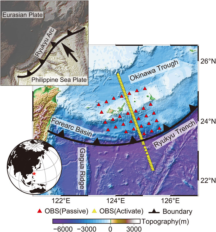
FIGURE 1. Locations of OBSs and land stations in the Ryukyu Trench, where the red and yellow triangles represent OBS (Passive) and OBS (Active), respectively, and the sawtooth line represents the plate boundary between the Eurasian Plate and the Pacific Plate (Plate boundary data from Nishizawa, (2009)).
Since Langston (1977) proposed the teleseismic receiver function method, it has gradually become one of the important methods to study the discontinuities in the interior of the Earth (Langston, 1977; Ammon et al., 1990). And Zhu And Kanamori, (2000) proposed the receiver function H-κ stacking method, it has become one of the most useful methods to obtain the crustal thickness and Vp/Vs ratio beneath stations. However, the current application of this technology is mostly limited to seismic data recorded by land stations. In recent years, with the rapid growth of broadband ocean bottom seismometers (OBSs), it is possible to further use this kind of response of seismic waves at discontinuities to image Earth’s interior beneath the ocean. For example, Audet (2016) discussed the feasibility and challenges of OBS receiver function research based on different synthetic receiver functions of marine lithosphere models. Guo et al. (2016) studied the structure of the lithosphere near the mid-ocean ridge and the characteristics of the mantle transition zone by using the OBS receiver function. Hu et al. (2016) obtained the velocity structures in the southwest sub-basin of the South China Sea by using the waveform inversion of the OBS receiver function. Geissler et al. (2017) conducted a detailed analysis of the waveform characteristics of OBS receiver functions with multiple Gaussian parameters and imaged mantle transition zone discontinuities under a hot-spot volcano of the South Atlantic Ridge.
Generally, the distribution of OBSs is very limited in oceanic areas, so it is difficult to comprehensively understand the geological evolution of the study area by using OBS seismic data alone. The wide coverage of gravity anomaly in oceanic areas can provide an important supplement for the study of regional crustal structure. In the gravity method, through spectral analysis of gravity anomaly data, the gravity anomaly corresponding to the Moho discontinuity could be separated from the total field for Moho inversion (Qin et al., 2011; Van der Meijde et al., 2013). However, anomalies at different depths with different densities can contribute to indistinguishable gravity anomalies near Earth’s surface. Only with more detailed prior information can the results from gravity inversion be reliable for further interpretation. Lowry and Pérez-Gussinyé (2011) proposed a method of joint inversion of receiver function and gravity, which can avoid the uncertainty of H-κ stacking because the Moho multiple waves in the receiver function are not easy to identify, to accurately estimate the crustal thickness and Vp/Vs in the western United States. Uieda And Barbosa, (2017) proposed a fast non-linear gravity inversion method to estimate the depth of Moho beneath the South American continent by combining satellite gravity data and seismological data. Shi et al. (2018) employed a standard algorithm of likelihood estimation to obtain the crustal thickness and Vp/Vs ratio, which were used to constrain the receiver function H-κ stacking result. The integration and joint interpretation of distinct geophysical datasets can be a highly effective approach for developing accurate and meaningful geological models (Roy et al., 2005).
The submarine geological survey is a challenging task, and it is of great significance to obtain the more accurate internal structure of the Earth by using geophysical data from the Ryukyu Trench. In this research, we combine the characteristics of receiver functions and gravity inversion. First, a delay term of the sedimentary layer is introduced into the H-κ stacking formula, and the sequential H-κ stacking method is used. As a result, the receiver function-based sequential H-κ stacking method can avoid the influence of the seafloor sedimentary layer. With the above methods, we can improve the stability of stacking results and obtain high-precision Moho depth points below the OBS. Furthermore, the high-precision Moho depth below the OBS is used as a constraint in Moho gravity inversion.
2 Regional geological background
As the plate boundary between the Eurasian Plate and the Philippine Sea Plate, it subducts at different angles from north to south Ryukyu (Figure 1). The Philippine Sea Plate subducted northwestward beneath the Eurasia Plate with an average velocity of about 8 cm/year (Yu et al., 1997). The Ryukyu Trench was subjected to strong extensional forces during the late Cretaceous, leading to the formation of a series of faults, rifts, and volcanic activity (Hong et al., 2020). During the Paleogene period, this region underwent intense compression and deformation, causing the crust to exhibit structural features similar to those seen today (Iwasaki et al., 1990). In the Neogene era, the northward movement of the Pacific Plate collided with the Eurasian Plate, leading to the formation of a series of geological structures, including the Ryukyu Trench, in the regions of the western Pacific Plate (Letouzey, 1985; Deschamps and Lallemand, 2003). The previous research has shown that during this period, the Ryukyu Trench underwent multiple active tectonic events, mainly characterized by the uplift and subsidence of seafloor mountains, the formation of faults and folds, and other phenomena (Zhang et al., 2020).
During the last fifty years, several seismic investigations have been carried out in the southern Ryukyu Trench (Murauchi et al., 1968; Henry et al., 1975; Carlson and Wilkens, 1983). Wang et al. (2004) combined the results of an OBS and a multichannel seismic recording system, showing the arc-parallel variation of the crustal structure in Ryukyu may be the consequence of west-increased lateral compression caused by the oblique sinking of the Philippine Sea Plate and collision with the Luzon Arc towards the northwestern border of the forearc (Wang et al., 2004). The knowledge of the crustal structure around the southernmost Ryukyu Trench has been greatly improved with the application of seismic surveys of the ocean bottom (Arai et al., 2017). The early seismic surveys mainly focused on eastern Taiwan with multichannel seismic reflection data and wide-angle OBS data. These studies revealed that the crust is usually 12 km–15 km thick (Wang et al., 2004; Nishizawa et al., 2009; Nishizawa et al., 2014). Arai et al. (2016) indicates that there is no conventional locked zone in the southern Ryukyu Trench, and that slow earthquakes are dominate at all depths. The presence of polarity reversals of seismic reflections and a low-velocity wedge above the plate suggests the presence of fluids at varying depths along the plate interface.
Even with the abovementioned seismic surveys, the regional crustal and lithosphere structure is still poorly understood due to the limited coverage of seismometers in Ryukyu Trench. Therefore, some researchers seek to combine different geophysical datasets with seismic data. By combining travel-time and gravity data, Roy et al. (2005) demonstrated that the joint interpretation of these two datasets is a useful tool for obtaining a more reliable subsurface geology model of the Ryukyu Trench. With the application of satellite gravity data and previous seismic data, the integration provides a good opportunity to recognize the crustal structure in the southernmost Ryukyu Trench. The passive-source OBSs are situated on the slope zone from the Ryukyu Island Arc to the south of the Ryukyu Trench (Figure 1). We combine the satellite gravity anomaly and OBS receiver function to obtain a more reliable crustal structure of the Ryukyu Trench. To provide geophysical foundation for researching the evolutionary process of convergence, disappearance, expansion and accretion of the Southeast Asian plate.
3 Methodology
3.1 Analysis of synthetic OBS receiver function
An OBS observation system is different from land stations; it is located on the seafloor so that it records vibrations. Thus, the air–sea interface above it can generate strong reflection (Liu et al., 2020). Such reflection will generate interlayer multiples and reverberation, which will cause certain interference to signal recorded by OBS vertical components. Because the radial receiver function is calculated by deconvolution between the radial component and the vertical component of the OBS, the air–sea surface reflection will distort the receiver function (Figure 2). At the same time, there are generally sedimentary layers on the seafloor, and the sediment–crust boundary is also an important discontinuity in the crust. When there is a sedimentary layer in the shallow part, in addition to converted and multiple waves due to the Moho surface, the sedimentary interface will generate another converted/reflected wave train when the incident teleseismic P-wave passes through it. In this case, the arrival time and amplitude of the Pmp phase in the receiver function will be affected.
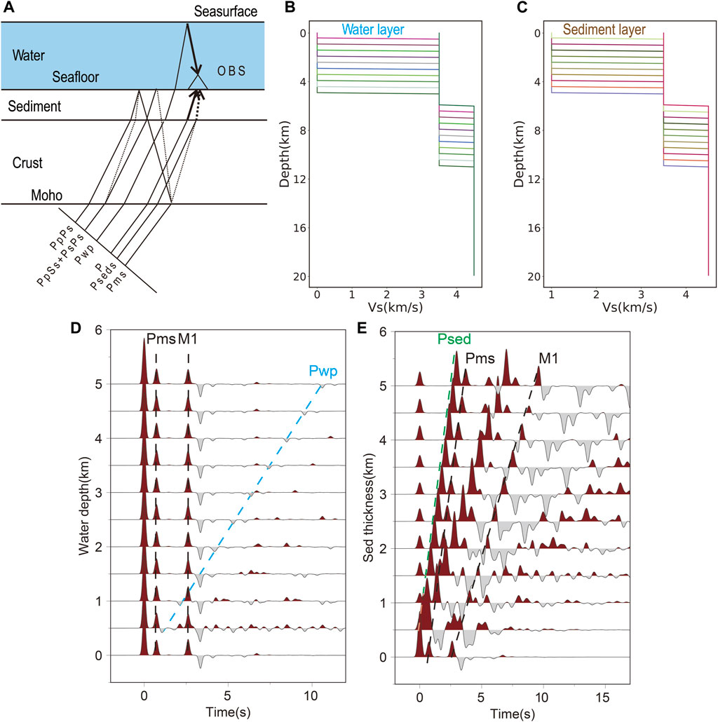
FIGURE 2. (A) The model with sediments and water layer. (B) The models with different water depth. (C) The models with different sediment thicknesses. (D) Synthetic receiver function of water model. (E) Synthetic receiver function of sediment model.
We have designed an ocean crust model containing a water layer or a sedimentary layer (Figures 2B, C) and synthesized theoretical seismograms based on the reflectivity method (Levin and Park, 1997a; Levin and Park, 1997b); then, the time-domain iterative deconvolution method is applied to the horizontal and vertical components to obtain the receiver function of these OBSs. Furthermore, according to the analysis of the influence of the seismic response of the sedimentary layer and the seawater layer on the OBS receiver function, a method suitable for obtaining the crustal structure of the sea area will be designed.
Figure 2B shows a series of models with different thicknesses of the water layer. The first layer is the mantle layer, where the S-wave velocity is 4.5 km/s, the P-wave velocity is 7.9 km/s, and the density is 4.0 g/cm3, and this layer is set as semi-infinite space. The second layer is the crust, where the S-wave velocity is 3.5 km/s, the P-wave velocity is 6.0 km/s, the density is 2.8 g/cm3, and the crustal thickness is set at 6 km (close to the average thickness of the global oceanic crust). The third layer is the water layer, where the P-wave velocity is 1.0 km/s, the S-wave velocity is 0 km/s, and the density is 1.1 g/cm3. The depth of the water layer is gradually stratified from 0 km to 5 km at intervals of 0.5 km for further synthetic tests. Figure 2C shows a series of velocity models with different sediment thicknesses. Similarly, the S-wave velocity, P-wave velocity, and density in the mantle are set as 4.5 km/s, 7.9 km/s, and 4.0 g/cm3, respectively, and the layer thickness is set as semi-infinite space. The S-wave velocity, P-wave velocity, and density in the crust are set as 3.5 km/s, 6.0 km/s, and 2.8 g/cm3, and the layer thickness is set as 6 km. The third layer is the sedimentary layer, with a P-wave velocity of 2.0 km/s, an S-wave velocity of 1.0 km/s, and a density of 2.5 g/cm3. The thickness of the sedimentary layer is gradually layered from 0 km to 5 km at intervals of 0.5 km.
Figure 2D shows that the synthetic receiver functions for different water depths and the Moho-converted waves and multiples in the receiver function are visible. Although there is the air–water interface surface reflection Pwp with negative amplitude (The ray path of this phase is shown in Figure 2A), the Pwp phase does not affect the arrival time of the relevant phase of the Moho. With the increase of water layer thickness, the arrival time of Pwp is regularly delayed. When the water depth is more than 2,000 m and the crustal thickness is more than 6 km, the main phases of the Moho in the receiver function will not directly interfere with Pwp (Figure 2D). Figure 2E shows the variation of the synthetic receiver function with the thickness of the sediment layer. When the seafloor sediment layer exists, a converted wave seismic phase P (sed) will be generated by the discontinuity at the bottom of the sediment layer (The ray path of this seismic phase is shown in Figure 2A). The amplitude and arrival time of Ps (Moho) and PpPs (Moho), PsPs, and PpSs (Moho) in the receiver function is affected by the Ps (Sed) and PpPs (Sed), PsPs, and PpSs (Sed). The arrival time of Ps (Moho) and Ps (Sed) is regularly delayed with the increase of the thickness of the seafloor sediment layer.
3.2 Sequential H-κ stacking method
The receiver function H-κ stacking method is one of the most commonly used methods to obtain the crustal thickness and Vp/Vs ratio beneath the station (Zhu and Kanamori, 2000). This method specifically uses the converted waves Ps and multiples waves PpPs, PsPs, and PpSs generated by the velocity discontinuity (Moho) in different receiver functions. By calculating the stacking amplitudes corresponding to the different crustal thickness and Vp/Vs ratio pairs, the crustal thickness and Vp/Vs ratio can be estimated by finding the parameters related to the maximum stacking amplitude.
The oceanic crust is generally thinner than the continental crust. To verify that the H-κ stacking method is applicable to estimate the thickness of the oceanic crust, we conducted a synthetic test. The crustal model and model parameters are shown in Figure 3A. We simulated 20 receiver functions with ray parameters ranging from 0.040 to 0.080 s/km (Figure 3B) (Generally, we could obtain high-quality receiver functions within this range for observed data) (Li et al., 2010). The results show that the crustal thickness is 6.01 km, and the Vp/Vs ratio is 1.71, which are consistent with the model values, indicating that the traditional H-κ stacking method can be used to accurately estimate the crustal thickness and Vp/Vs ratios of the oceanic crust (Figure 3C).
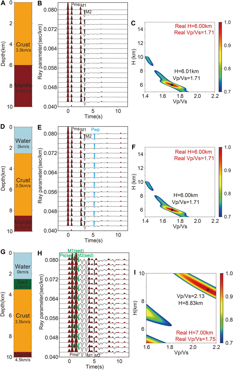
FIGURE 3. (A), (D), and (G) Crustal model. (B), (E), and (H) Synthetic receiver functions. (C), (F), and (I) H-κ stacking result.
The major difference between the receiver function observed by OBSs and land stations is that there is a water layer above the observation station. Therefore, we designed a crustal model with water to verify the H-κ stacking method can correctly calculate the crustal thickness (The parameters of the model are shown in Figure 3D). It can be seen that the Pwp will not interfere with the Ps (Moho) and PpPs (Moho), PsPs, and PpSs (Moho). The H-κ stacking results are consistent with the true values, indicating that the Pwp will not significantly affect the H-κ stacking results (Figure 3).
In addition, sedimentary layers are widespread in the ocean. As mentioned in Section 3.1, the multiples from the sedimentary layer will be mixed with the Moho-related phases, which leads to a cycle-skipping effect in the H-κ analysis. To test the sedimentary layer effects for H-κ stacking, we conducted a synthetic test with the model parameters presented in Figure 3G. The H-κ stacking result shows that the crustal thickness is 8.83 km, different from the true value (7.00 km), indicating that the estimated thickness due to the existence of a sedimentary layer in the traditional H- κ stacking method is not negligible.
To eliminate the influence of the sedimentary layer in H-κ stacking, we attempt to use the sequential H-κ stacking method. Specifically, the strategy of two-step stacking is adopted:
For the first stacking, we seek to estimate the thickness and the Vp/Vs ratio of the sedimentary layer. The P-wave velocity in the stack is assumed to be the sedimentary layer velocity Vp (sed), and the thickness H (sed) and Vp/Vs ratio of the sedimentary layer κ (sed) are estimated by the arrival time difference of the three seismic phases with respect to the direct P-wave (Formulas 1–3). The arrival time difference for each H-κ pair is substituted into Formula 7 to compute the first stacking function (Zhu And Kanamori, 2000).
where
where
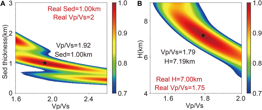
FIGURE 4. Sequential H-κ stacking of synthetic receiver functions of the crustal model with a sedimentary layer. (A) Sedimentary thickness and (B) Moho depth.
3.3 Gravity inversion constrained by receiver function
Thus far, the above sequential H-κ stacking method has been able to avoid the effect of sediments and to accurately obtain the Moho depth beneath the OBS. However, the deployment cost of an OBS is relatively high compared with that of land stations, and the deployment conditions are more stringent, resulting in limited data coverage. Therefore, the limited sampling of the Moho undulation obtained by sequential H-κ stacking brings difficulties to the subsequent geological interpretation. The gravity anomaly data have the characteristics of high coverage, but due to the superimposition of gravity anomalies, the gravity inversion is non-unique. Therefore, to solve the problem of insufficient OBS coverage and multiple solutions of traditional gravity inversion, a gravity inversion method based on the Moho surface constrained by high-precision Moho depth points under the OBS is proposed in this study. The inversion objective function
where
where
Figure 5A shows that reference Moho and Moho together form the integral interval of gravity anomaly, so the selection of reference Moho depth is very important to gravity Moho inversion. However, the reference Moho depth cannot be directly obtained from gravity data. In this study, we use tesseroids structures to model the Moho and compute numerically the effects of the Moho anomalies (Figure 5B) (Uieda et al., 2016). The integral formula of the theoretical gravity anomaly in observation point based on geocentric coordinate system is as follows (Formula 10) (Uieda and Barbosa, 2017).
where
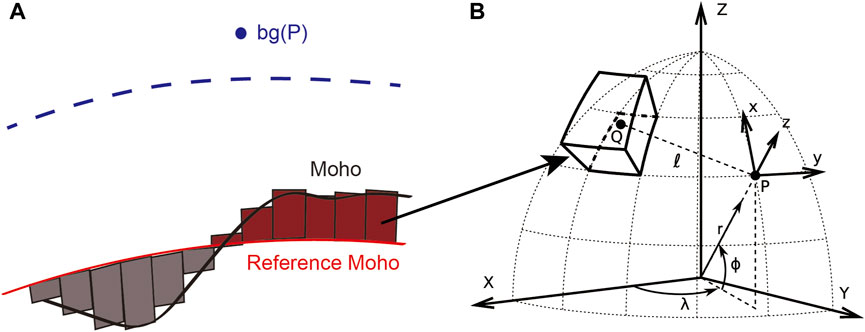
FIGURE 5. The calculation of theoretical gravity anomaly. (A) The discretization of the anomalous Moho (The grey block represents a negative density; The red block represents a positive density; The black line represents Moho; The red line represents the reference Moho); (B) The geocentric coordinate system [The P is the observation point and the Q is the integration point (Uieda et al., 2016)].
Since the reference Moho depth is unknown, we usually use prior information to set an approximate range. We then use the Moho depth obtained from sequential H-κ stacking to estimate the depth of reference Moho. The cross-validations are conducted to select the reference Moho depth. In synthetic test, we set the
where
i) Giving the variation range of the possible of
ii) Traversing each reference value (
For
For
Perform gravity inversion;
Calculate MSE (Formula 11); Done; Done;
iii) Returning the reference value (
Through the search of the above processes, we can obtain the optimal reference Moho depth. Based on the value of these optimal super-parameters, we conduct the gravity inversion to obtain the Moho depth. To verify the effectiveness of the above method, we designed a Moho model that fluctuates sinusoidally for synthetic tests (Figure 6A). Compared with the traditional gravity inversion method, our method can recover the Moho closer to the real model (Figures 6B, C). In addition, the distribution of the standard deviation and mean value of gravity anomaly residual data are both the same (Figure 7A), which also shows that gravity inversion has strong non-uniqueness. The unconstrained errors are concentrated at around 4 km–6 km, indicating that the inversion results are generally biased (Figure 7B). However, the inversion results based on control points are closer to the real model, which further shows that the gravity inversion with control points with high accuracy can effectively improve the accuracy of Moho inversion (Figure 7B).
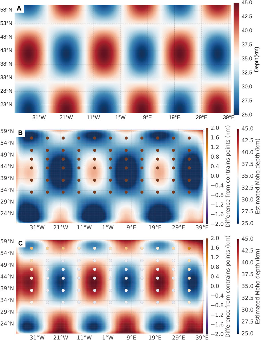
FIGURE 6. Checkboard resolution tests for gravity inversion. (A) Moho depth model. (B) Result of gravity inversion. (C) Result of gravity inversion based on control point constraint (The dots indicate the location of the OBS. The color of the dots indicates the difference between the constrained points value and the inversion result).
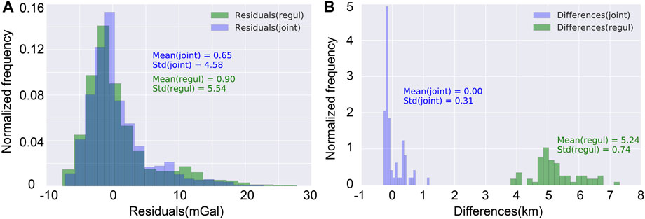
FIGURE 7. Comparison of inversion residuals. (A) Statistical comparison of residual error of gravity anomaly data recovered by inversion model. (B) Statistical comparison of Moho depth error of inversion model.
4 Gravity inversion constrained by OBS RFs in the Ryukyu Trench
We applied seismic data recorded by 30 OBSs near the Ryukyu Trench on the JAMSTEC (www.jamstec.go.jp), including continuous seismic records from 23 November 2013, to 18 February 2014 (Because of some errors in L02 and L16, we ultimately succeeded in obtaining seismic data recorded by 28 OBSs). We organized 44 earthquakes in the catalog with a magnitude above 5.5 and epicenter distances between 30°C and 90°C (https://www.usgs.gov). Before the receiver function calculation, we perform some preprocessing on the original seismic data, including removing the mean, removing the linear trend and filtering. By analyzing the frequency bands affected by the interference noise of the OBS on the seafloor, band-pass filtering with different frequency bands is applied to the raw seismic data. Specifically, the first group of seismic data uses a filtering frequency band of 0.1 Hz–2.0 Hz, which is selected because of the main frequency of the P-wave in the range of 0.3 Hz–2.0 Hz. Through this frequency band, more complete frequency information can be retained, which is very helpful to study the crustal interface by using the Moho Ps transform seismic facies, and the high-frequency component will be more detailed in describing the structure of shallow sedimentary layers. The second group uses a frequency band of 0.03 Hz–1.0 Hz. As the seafloor noise of the original data is mainly concentrated within 1.0 Hz–3.0 Hz, the noise can be removed through filtering in this frequency band to improve the signal-to-noise ratio.
Then, we use the time domain iterative deconvolution method to calculate the receiver function (Ligorría and Ammon, 1999). A Gaussian filter with a coefficient of 2.5 was used to filter receiver functions. Taking YA.L01 as an example, we calculate the receiver functions based on manually selecting the receiver functions with high signal-to-noise ratio and clear seismic phase. We set the Sedimentary thickness search range of 0–3 km and step size of 0.1. The κ search range of 1.5–3.0 used a step size of 0.01 (Crustal thickness range of 15 km–30 km and κ search range of 1.6–2.0). For the first stacking weights of three seismic phases [Ps (Sed) and PpPs (Sed), PsPs, and PpSs (Sed)] were 0.4, 0.4, and 0.2 respectively. For the second stacking weights [Ps (Moho) and PpPs (Moho), PsPs, and PpSs (Moho)] were 0.5, 0.3, and 0.2 respectively. The result of sequential H-κ stacking at YA.L01 shows in Figure 8.
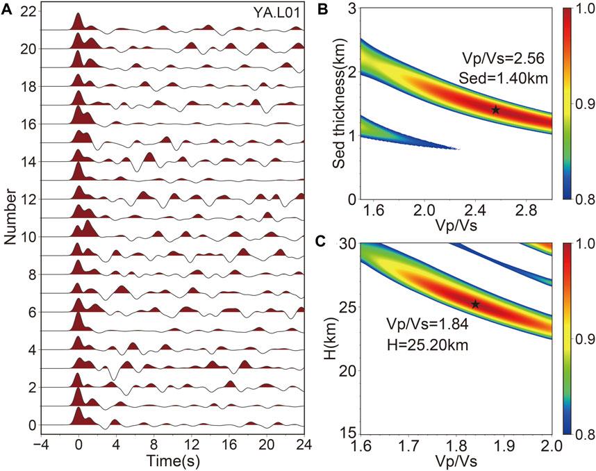
FIGURE 8. (A) OBS receiver functions, (B) sedimentary thickness, and (C) and Moho depth of sequential H-κ stacking at OBS site L01.
Based on teleseismic data recorded by the 28 OBSs near the Ryukyu Trench, we obtained reasonable values of sedimentary layer and crustal thicknesses by sequential H-κ stacking (Figure 9). At the same time, to verify the results, we also downloaded the sedimentary layer and crustal thicknesses in the Ryukyu Trench in the CRUST1.0 model (Laske et al., 2012). It can be seen from the comparison that the thickness distribution of the sedimentary layer obtained by sequential H-κ stacking is consistent with that of the CRUST1.0 model (Figures 9A, C). The thickness of the sedimentary layer decreases gradually from north to south, and that in overall study area is about 1 km. The study area’s thickest and thinnest sedimentary layers exist at stations L07 at the northernmost region and L28 at the southernmost region. Because the two stations are located at island arcs and trenches, they are consistent with the geological structure of the corresponding areas of the stations. Because the resolution of the CRUST1.0 model is 1°C × 1°C, its resolution is still low relative to the distribution density of OBSs in the study area. Therefore, by using the thickness distribution of the sedimentary layer obtained by sequential H-κ stacking, we can depict more detailed thickness change and spatial distribution of the sedimentary layer in the study area. The crustal thickness distribution of sequential H-κ stacking and the CRUST1.0 model show a decreasing trend from north to south, which is also obviously divided into three steps (compared with Figures 9B, D). Due to the higher resolution, the thickness distribution of the sedimentary layer and crustal thickness obtained by superposition can more carefully depict the crustal structure changes in the study area while maintaining accuracy and precision.
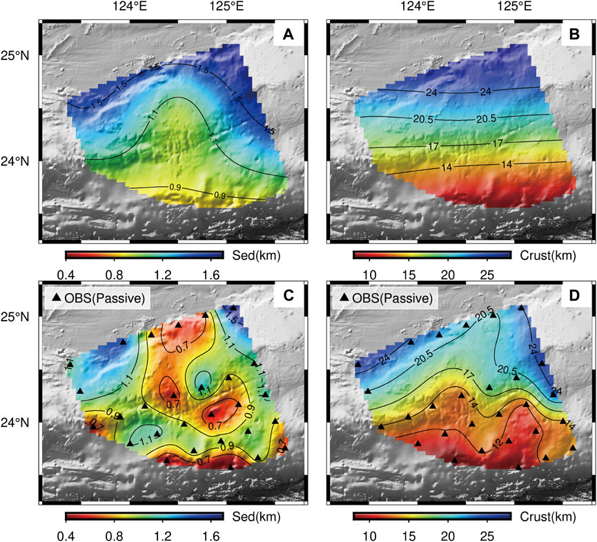
FIGURE 9. (A) and (B) Distribution map of sedimentary layer and crustal thickness with CRUST1.0 model (Laske et al., 2012), respectively. (C) and (D) Distribution map of sedimentary layer and crustal thickness obtained by sequential H-κ stacking.
The Moho is also one of the main density difference interfaces within Earth, so we can also use gravity inversion to obtain Moho undulations. Gravity anomaly data is the summed gravitational response of all anomalous bodies’ densities below the Earth’s surface. In general, the anomalous responses from small-scale or shallow-density anomalous bodies and large-scale or deep-density anomalous bodies exhibit significant differences in the frequency spectrum. We can be separated using frequency analysis to distinguish gravity anomaly sources at different depths. We filter the original gravity data, eliminate and suppress the noise interference, and also eliminate the gravity response of shallow non-uniform anomalies, to separate the overlapping local anomalies. Before the inversion of Moho undulation characteristics by gravity anomaly, it is necessary to separate the original gravity anomaly data to obtain the gravity anomaly response reflecting Moho undulation characteristics (Chu et al., 2022).
We use the Bouguer gravity anomaly in the Ryukyu Trench area from WGM 2012 (data accuracy is 2′×2′) (Bostock and Trehu, 2012). Filtering can suppress noise and unrelated anomalies in the raw gravity data (Van der Meijde et al., 2013). We filter the gravity anomaly before inversion and the low-pass filtering wavelength is selected to be 20 km. After filtering, most of the high-frequency noise is removed, and the gravity anomaly data that only reflect the undulating characteristics of Moho are extracted (Figure 10A). Based on the above gravity anomaly, the Moho undulation characteristics in the Ryukyu Trench area are obtained by gravity inversion (Figure 10B).

FIGURE 10. (A) Bouguer gravity data after filtering. (B) Moho depth calculated by gravity inversion (only) in the Ryukyu Trench.
We take the result of sequential H-κ stacking as the constraint to gravity inversion and obtained the overall Moho undulation characteristics near the Ryukyu Trench (Figure 11A). We set the
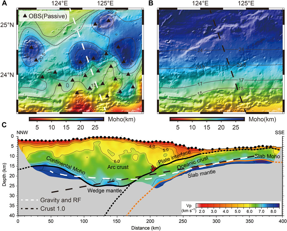
FIGURE 11. (A) Moho depth calculated by gravity inversion constrained by receiver function in the Ryukyu Trench. (B) Distribution map of crustal thickness with CRUST1.0 model (Laske et al., 2012). (C) Seismic reflection profile of active source line [Arai et al. (2016), modified] [The white dotted line represents Moho depth obtained by gravity inversion constrained by receiver function; The black dotted line represents Moho depth from CRUST1.0 (Laske et al., 2012)].
The Moho depth distribution of gravity inversion constrained by the receiver function shows the overall characteristics of thick crust in the north and thin crust in the south of the Ryukyu Trench subduction zone. The overall characteristics are basically similar to CRUST1.0 model (Figures 11A, B). The average depth of the Moho is about 17 km. The Moho near the subduction zone shows an obvious deepening trend (Figure 11A). Figure 11C shows that the depth of Moho surface gradually deepens from Slab mantle to Wedge mantle, and then shallow again at Continental Moho. The result of gravity inversion constrained by the receiver function shows overall characteristics of Moho surface affected by subduction zone. Due to the dense layout of active source OBS lines and high data signal-to-noise ratio, its results have high resolution. The undulating pattern of the Moho is consistent with that of the seismic reflection profile in the corresponding region (Audet, 2016), which verifies the rationality of the results (Figure 11C).
5 Discussion
In comparison with the previous crustal structure developed by Wang et al. (2004), who performed layer-stripping Monte Carlo inversion of P velocity model from OBS/MCS profiles, they showed an 8 km–15 km thickness beneath the forearc basins, in excellent agreement with our results (Southeast of the study area in Figure 11A). The Ryukyu arc basement is 20 km–25 km thick north of the forearc basins, which is also generally consistent with our results (Middle of the study area in Figure 11A). Arai et al. (2016) presented reflection data from MCS and refraction/wide-angle reflection data from OBS records, providing a consistent and distinct image of the Philippine Sea slab subducting from the trench to a depth of ∼25 km, which is similar to our results (The white dotted line in Figure 11C indicates the Moho depth of our results). Along the Manila Trench, the Eurasian Plate subducts and accretes beneath the Philippine Plate (Chen et al., 2014). In the Ryukyu Trench, the subduction is in the opposite direction, where the Philippine Plate subducts beneath the Eurasian Plate (Kodaira et al., 1996). We believe that the subduction accretion and collision between plates control the deformation characteristics of the Moho surface in the Ryukyu Trench.
Due to the higher resolution of the active seismic profile, we can find that there is a thicker sedimentary thickness in fore-arc. And the sedimentary layer structure of the active seismic profile exhibits significant fluctuations from southeast to northwest. Although there are significant differences in absolute depth, the fluctuation trend is basically consistent with the active source, and it also has better resolution compared to CRUST1.0 model. It can be seen from the distribution of the thickness of the sedimentary layer (Figure 9C) that during the transition from the Ryukyu Trench to the island arc, the thickness of the sedimentary layer and the crust increased along the NNW subduction direction (Suenaga et al., 2021). This thickening phenomenon may be due to the accumulation of some sedimentary structures caused by subduction. The bottom interface of the sedimentary layer in the arc shell area presents a strong undulating structure, which also shows that the thickness of the sedimentary layer increases and decreases alternately from southeast to northwest. We believe that this region underwent intense compression and deformation in the Paleogene period showing folding mode from the bottom of the trench to the top of the arc shell (Iwasaki et al., 1990).
In this study, the Moho undulations with higher resolution and wider coverage are obtained by using sequential H-κ stacking results to constrain gravity inversion, which shows that the Moho on the southern edge of the Ryukyu Trench subduction zone is shallow and belongs to an oceanic crust nature; the Moho in the north edge is deep and belongs to a continental crust (Arai et al., 2016) (Figure 11C). The main feature of the Moho along the subduction zone from SE to NW is first thickening and thinning, which verifies the subduction direction of the Philippine Sea Plate to the Eurasian Plate (NNW) (Figures 11A, C). Moreover, this strongly undulating Moho surface and sedimentary layer structure may be the comprehensive result of multiple complex tectonic evolutions.
6 Conclusion
Aiming at investigating the influence of the water layer and sediment layer on the OBS receiver function, this study designed sequential H-κ stacking, and high precision Moho depth points under the OBSs are obtained. On this basis, the depth information of the Moho below the OBSs is taken as the control point, and a gravity Moho inversion method constrained by the OBS receiver function is proposed. Based on OBS observation data of 28 stations and Bouguer gravity anomaly data, we obtained the characteristics of Moho fluctuation near the Ryukyu Trench. The main conclusions are as follows:
(1) Compared with the receiver function method, our method has better constraints in areas lacking station coverage and avoids the uncertainty caused by interpolation between stations. Compared with gravity inversion, the constraint of seismic data can reduce the non-uniqueness of gravity inversion—the undulation characteristics of Moho inversion results are more refined, local anomalies are better reflected, and the horizontal spatial coverage and vertical spatial resolution requirements are satisfied.
(2) Using the gravity inversion method constrained by the OBS receiver function, we determined that the Moho depth of the Ryukyu Trench varies from 15 km to 20 km, and the Philippine Sea Plate subduction area shows an obvious Moho deep anomaly, showing that the southern edge of the Ryukyu Trench belongs to oceanic crust, whereas the northern edge belongs to continental crust, revealing that the crustal thickness of the Ryukyu Trench area thickens along the NNW subduction direction and that the subduction direction of the Philippine Sea Plate is from SE to NW.
Data availability statement
The original contributions presented in the study are included in the article/supplementary material, further inquiries can be directed to the corresponding authors.
Author contributions
TY wrote the first draft of the manuscript. YX and TX contributed to the conception and design of the study. ND, FN, WC, DC, CL, and TH wrote sections of the manuscript. All authors contributed to the manuscript revision and read and approved the submitted version.
Funding
This work was supported by the National Natural Science Foundation of China under grant numbers 91858212, 42074092, 42130807, and 42006062.
Acknowledgments
We would like to express our sincere appreciation and deep-felt memory to our former group leader and good friend, Prof. Zhongjie Zhang, who suddenly passed away ten year ago (September 6, 2013). Thanks to Japan Agency for Marine Earth Science and Technology for providing seismic data for this study (www.jamstec.go.jp). All Figures in this study are plotted by the GMT and Matplotlib: Visualization with Python (http://gmt.soest.hawaii.edu/home/ and https://matplotlib.org/).
Conflict of interest
The authors declare that the research was conducted in the absence of any commercial or financial relationships that could be construed as a potential conflict of interest.
Publisher’s note
All claims expressed in this article are solely those of the authors and do not necessarily represent those of their affiliated organizations, or those of the publisher, the editors and the reviewers. Any product that may be evaluated in this article, or claim that may be made by its manufacturer, is not guaranteed or endorsed by the publisher.
References
Ammon, C. J., Randall, G. E., and Zandt, G. (1990). On the nonuniqueness of receiver function inversions. J. Geophys. Res. Solid Earth 95, 15303–15318. doi:10.1029/JB095iB10p15303
Arai, R., Kodaira, S., Yamada, T., Takahashi, T., Miura, S., Kaneda, Y., et al. (2017). Subduction of thick oceanic plateau and high-angle normal-fault earthquakes intersecting the slab. Geophys. Res. Lett. 44, 6109–6115. doi:10.1002/2017GL073789
Arai, R., Takahashi, T., Kodaira, S., Kaiho, Y., Nakanishi, A., Fujie, G., et al. (2016). Structure of the tsunamigenic plate boundary and low-frequency earthquakes in the southern Ryukyu Trench. Nat. Commun. 7, 12255–12257. doi:10.1038/ncomms12255
Audet, P. (2016). Receiver functions using OBS data: Promises and limitations from numerical modelling and examples from the cascadia initiative. Geophys. J. Int. 205, 1740–1755. doi:10.1093/gji/ggw111
Bostock, M., and Trehu, A. (2012). Wave-field decomposition of ocean bottom seismograms. Bull. Seismol. Soc. Am. 102, 1681–1692. doi:10.1785/0120110162
Carlson, R., and Wilkens, R. (1983). Seismic crustal structure and the elastic properties of rocks recovered by drilling in the Philippine Sea. Geodyn. West. Pacific-Indonesian Region 11, 127–136. doi:10.1029/GD011p0127
Chen, C. X., Wu, S. G., and Zhao, C. L. (2014). Incoming plate variation along the northern Manila Trench. Chin. J. Geophys. (in Chinese) 57 (12), 4063–4073. doi:10.6038/cjg20141218
Chu, W., Xu, Y., and Hao, T. Y. (2022). Moho structure in Sulawesi area based on spherical gravity inversion. Chinese Journal of Geophysics (in Chinese) 65, 2198–2209. doi:10.6038/cjg2022P0148
Deschamps, A., and Lallemand, S. (2003). Geodynamic setting of Izu-Bonin-Mariana boninites. Geological Society, London, Special Publications 219 (1), 163–185. doi:10.1144/GSL.SP.2003.219.01.08
Gao, X. L. (2003). Tectonics and motion of the Ryukyu trench. Progress in Geophysics 18 (2), 293–301. doi:10.3969/j.issn.1004-2903.2003.02.018
Geissler, W. H., Jokat, W., Jegen, M., and Baba, K. (2017). Thickness of the oceanic crust, the lithosphere, and the mantle transition zone in the vicinity of the Tristan da Cunha hot spot estimated from ocean-bottom and ocean-island seismometer receiver functions. Tectonophysics 716, 33–51. doi:10.1016/j.tecto.2016.12.013
Guo, Y. L., Hu, H., Ruan, A. G., and Wei, X. D. (2016). The significance and methods of OBS receiver function. South China of Journal of Seismology (in Chinese) 36 (4), 20–26. doi:10.13512/j.hndz.2016.04.004
Henry, M., Karig, D., and Shor, G. (1975). Two seismic refraction profiles in the west Philippine Sea. DSDP 31, 611–614. doi:10.2973/dsdp.proc.31.128.1975
Hong, W. T., Yu, M. G., Yang, Z. L., and Xing, G. F. (2020). Cenozoic tectonic units and their stratigraphic characteristics of southern west Pacific region: Implication for Himalayan orogeny. Geological Bulletin of China 39 (6), 839–860. doi:10.12097/j.issn.1671-2552.2020.06.005
Hu, H., Ruan, A. G., You, Q. Y., Li, J. B., Hao, T. Y., and Long, J,P. (2016). Using OBS teleseismic receiver functions to invert lithospheric structure —a case study of the southwestern subbasin in the South China sea. Chinese Journal of Geophysics (in Chinese) 59 (4), 1426–1434. doi:10.6038/cjg20160423
Iwasaki, T., Hirata, N., Kanazawa, T., Melles, J., Suyehiro, K., Urabe, T., et al. (1990). Crustal and upper mantle structure in the Ryukyu island arc deduced from deep seismic sounding. Geophysical Journal International 102 (3), 631–651. doi:10.1111/j.1365-246X.1990.tb04587.x
Kodaira, S., Iwasaki, T., Urabe, T., Kanazawa, T., Egloff, F., Makris, J., et al. (1996). Crustal structure across the middle Ryukyu trench obtained from ocean bottom seismographic data. Tectonophysics 263, 39–60. doi:10.1016/S0040-1951(96)00025-X
Langston, C. A. (1977). Corvallis, Oregon, crustal and upper mantle receiver structure from teleseismic P and S waves. Bulletin of the Seismological Society of America 67, 713–724. doi:10.1785/BSSA0670030713
Laske, G., Masters, G., Ma, Z., and Pasyanos, M. E. (2012). “CRUST1.0: An updated global model of Earth's crust,” in EGU General Assembly Conference Abstracts, Vienna, Austria, 7-12 April, 2013.
Letouzey, J., and Kimura, M. (1985). Okinawa Trough Genesis: Structure and evolution of a backarc basin developed in a continent. Marine and Petroleum Geology 2 (2), 111–130. doi:10.1016/0264-8172(85)90002-9
Levin, V., and Park, J. (1997a). Crustal anisotropy in the Ural Mountains foredeep fromteleseismic receiver functions. Geophysical Research Letters 24, 1283–1286. doi:10.1029/97GL51321
Levin, V., and Park, J. (1997b). P-SH conversions in a flat-layered medium withanisotropy of arbitrary orientation. Geophysical Journal International 131, 253–266. doi:10.1111/j.1365-246X.1997.tb01220.x
Li, X., and Götze, H.-J. (2001). Ellipsoid, geoid, gravity, geodesy, and geophysics. Geophysics 66, 1660–1668. doi:10.1190/1.1487109
Li, Z., Hao, T., Xu, Y., Xu, Y., and Roecker, S. (2010). A global optimizing approach for waveform inversion of receiver functions. Computers & geosciences 36, 871–880. doi:10.1016/j.cageo.2009.11.007
Ligorría, J. P., and Ammon, C. J. (1999). Iterative deconvolution and receiver-function estimation. Bulletin of the seismological Society of America 89 (5), 1395–1400. doi:10.1785/BSSA0890051395
Liu, Y., Liu, B., Liu, C., and Hua, Q. (2020). The crustal structure of the eastern subbasin of the South China sea: Constraints from receiver functions. Geophysical Journal International 222, 1003–1012. doi:10.1093/gji/ggaa246
Lowry, A. R., and Pérez-Gussinyé, M. (2011). The role of crustal quartz in controlling Cordilleran deformation. Nature 471, 353–357. doi:10.1038/nature09912
Murauchi, S., Den, N., Asano, S., Hotta, H., Yoshii, T., Asanuma, T., et al. (1968). Crustal structure of the Philippine Sea. Journal of Geophysical Research 73, 3143–3171. doi:10.1029/JB073i010p03143
Nishizawa, A. (2009). Fault model of the 1771 Yaeyama earthquake along the Ryukyu Trench estimated from the devastating tsunami. Geophysical Research Letters 36, L19307. doi:10.1029/2009GL039730
Nishizawa, A., Kaneda, K., Katagiri, Y., and Oikawa, M. (2014). Wide-angle refraction experiments in the Daito Ridges region at the northwestern end of the Philippine Sea plate. Earth, Planets and Space 66, 25–16. doi:10.1186/1880-5981-66-25
Nishizawa, A., Kaneda, K., and Oikawa, M. (2009). Seismic structure of the northern end of the Ryukyu Trench subduction zone, southeast of Kyushu, Japan. Earth, Planets and Space 61, e37–e40. doi:10.1186/BF03352942
Qin, J. X., Hao, T. Y., Xu, Y., Huang, S., Lv, C. C., and Hu, W. J. (2011). The distribution characteristics and the relationship between the tectonic units of the Moho depth in south China Sea and adjacent areas[J]. Chinese Journal of Geophysics (in Chinese) 54 (12), 3171–3183. doi:10.3969/j.issn.0001-5733.2011.12.017
Roy, L., Sen, M. K., McIntosh, K., Stoffa, P. L., and Nakamura, Y. (2005). Joint inversion of first arrival seismic travel-time and gravity data. Journal of Geophysics and Engineering 2, 277–289. doi:10.1088/1742-2132/2/3/011
Seno, T., Stein, S., and Gripp, A. E. (1993). A model for the motion of the Philippine Sea plate consistent with NUVEL-1 and geological data. Journal of Geophysical Research Solid Earth 98, 17941–17948. doi:10.1029/93jb00782
Shen, Z. K., Zhao, C., Yin, A., Li, Y., Jackson, D. D., Fang, P., et al. (2000). Contemporary crustal deformation in East Asia constrained by Global Positioning System measurements. Journal of Geophysical Research Solid Earth 105, 5721–5734. doi:10.1029/1999JB900391
Shi, L., Guo, L., Ma, Y., Li, Y., and Wang, W. (2018). Estimating crustal thickness and Vp/Vs ratio with joint constraints of receiver function and gravity data. Geophysical Journal International 213, 1334–1344. doi:10.1093/gji/ggy062
Silva, J. B., Medeiros, W. E., and Barbosa, V. C. (2001). Potential-field inversion: Choosing the appropriate technique to solve a geologic problem. Geophysics 66, 511–520. doi:10.1190/1.1444941
Suenaga, N., Yoshioka, S., and Ji, Y. F. (2021). 3-D thermal regime and dehydration processes around the regions of slow earthquakes along the Ryukyu Trench. Scientifc Reports 11, 11251. doi:10.1038/s41598-021-90199-2
Uieda, L., and Barbosa, V. C. (2017). Fast nonlinear gravity inversion in spherical coordinates with application to the South American Moho. Geophysical Journal International 208, 162–176. doi:10.1093/gji/ggw390
Uieda, L., Barbosa, V. C. F., and Braitenberg, C. (2016). Tesseroids: Forward-modeling gravitational fields in spherical coordinates. Geophysics 81, F41–F48. doi:10.1190/geo2015-0204.1
Van der Meijde, M., Julià, J., and Assumpção, M. (2013). Gravity derived Moho for south America. Tectonophysics 609, 456–467. doi:10.1016/j.tecto.2013.03.023
Wang, T. K., Lin, S. F., Liu, C. S., and Wang, C. S. (2004). Crustal structure of the southernmost Ryukyu subduction zone: OBS, MCS and gravity modelling. Geophysical Journal International 157, 147–163. doi:10.1111/j.1365-246X.2004.02147.x
Yeck, W. L., Sheehan, A. F., and Schulte-Pelkum, V. (2013). Sequential H- stacking to obtain accurate crustal thicknesses beneath sedimentary basins. Bulletin of the Seismological Society of America 103, 2142–2150. doi:10.1785/0120120290
Yu, S. B., Chen, H. Y., and Kuo, L. C. (1997). Velocity field of GPS stations in the Taiwan area. Tectonophysics 274, 41–59. doi:10.1016/S0040-1951(96)00297-1
Zhang, Y., Yao, Y. J., Li, X. J., Shang, L. N., Yang, C. P., Wang, Z. B., et al. (2020). Tectonic evolution and resource-environmental effect of China Seas and adjacent areas under the multisphere geodynamic system of the East Asia ocean-continent convergent belt since Mesozoic. Geology in China 47 (5), 1271–1309.
Keywords: gravity inversion, ocean bottom seismometer, receiver function, Ryukyu Trench, H-κ stacking
Citation: Yang T, Xu Y, Du N, Xu T, Cao D, Nan F, Chu W, Liang C and Hao T (2023) Gravity inversion constrained by OBS receiver function reveals crustal structure in Ryukyu Trench. Front. Earth Sci. 11:1187683. doi: 10.3389/feart.2023.1187683
Received: 16 March 2023; Accepted: 11 April 2023;
Published: 20 April 2023.
Edited by:
Xiaoyu Guo, Sun Yat-sen University, ChinaReviewed by:
Yongqian Zhang, Chinese Academy of Geologi-cal Sciences (CAGS), ChinaYonghua Li, China Earthquake Administration, China
Copyright © 2023 Yang, Xu, Du, Xu, Cao, Nan, Chu, Liang and Hao. This is an open-access article distributed under the terms of the Creative Commons Attribution License (CC BY). The use, distribution or reproduction in other forums is permitted, provided the original author(s) and the copyright owner(s) are credited and that the original publication in this journal is cited, in accordance with accepted academic practice. No use, distribution or reproduction is permitted which does not comply with these terms.
*Correspondence: Tingwei Yang, dHd5YW5nQG1haWwuaWdnY2FzLmFjLmNu