Data processing method for magnetotelluric sounding based on cepstral analysis

Magnetotelluric (MT) signals exhibit the characteristics of being weak and having a wide frequency band. The acquired field data are susceptible to various types of noise, which poses challenges in accurate identification and processing. Currently, there exist numerous MT data processing methods; however, they lack efficiency and physical meaning. To address this issue and improve the signal-to-noise ratio of the acquired data, this study proposes a MT data processing method based on cepstral analysis. By employing cepstral analysis on the MT data, the cepstrum is obtained, and an appropriate truncation position is selected for processing. The experimental results demonstrate that this method obtains smoother and more continuous apparent resistivity curves with fewer errors. Compared with other methods, the cepstral analysis method can effectively suppress different types of MT noise, and the method is simple and efficient with clear physical significance.

1 Introduction

The magnetotelluric (MT) method is an electromagnetic exploration method that was first proposed in the 1950s (Tikhonov 1950; Cagniard, 1953). Due to its advantages of low cost, simple construction, large detection depth, and high resolution of low-resistivity layers, the method is widely used in exploration geophysics. However, the natural MT signal is extremely weak, and its frequency band is extremely wide; this makes such signals with nonlinear and nonstationary characteristics more susceptible to interference by various noises (Wang and Wang, 2004a; Wang, 2004b). With the continuous advancement of human civilization, electromagnetic interference caused by human and industrial activities has become increasingly severe, resulting in a typical near-source effect in the collection of MT data in the field (Wei, 2002). Whether studying deep geological formations or exploring mineral resources, it is impossible to completely avoid the complex electromagnetic interference environment (Dong et al., 2012). Noise suppression is always an research hot spot in MT studies. To address this problem, geophysicists have proposed a series of techniques to obtain unbiased MT impedance data.

The traditional least squares method assumes that the input is not affected by noise and that the noise at the output follows a Gaussian distribution. The time series of MT data are assumed to be stationary. However, MT signals are actually nonstationary due to various factors, such as geomagnetic storms and anthropogenic noise. Due to the presence of measurement errors and non-unique sources, the data may contain large outliers, resulting in lower fitting accuracy (Gangi and Shapiro, 1979). In this regard, Gamble et al. (1979) proposed the remote reference method for the first time, which involves adding remote reference points and utilizing cross-power spectra instead of auto-power spectra to suppress unrelated noise in MT data. However, its effectiveness in the low-frequency range is not optimal. Ritter et al.(1998) utilized indicators such as the transfer function between the magnetic field at measurement and reference points to determine the presence of noise in each data segment. They removed the segments with noise before the subsequent impedance estimation to eliminate their impact. To suppress non-Gaussian noise, the robust method has been widely applied for transfer function (TF) correction (Egbert and Booker, 1986; Chave et al., 1987; Chave and Thomson, 1989), where coefficients are weighted to eliminate the influence of outliers. Although this method can achieve smooth apparent resistivity and phase curves within a certain frequency band, its effectiveness is mainly limited to the high-frequency range. Satisfactory results are often challenging to obtain in the low-frequency range due to the limited sampling rate. Therefore, neither the remote reference method nor the robust estimation method can fully solve the challenges associated with processing MT data.

Consequently, several signal processing and inversion methods have been introduced into the field of MT data processing. Interpolation, filtering, and regularization techniques such as smoothing constraints have played crucial roles as preprocessing algorithms. Among these techniques, time- and frequency-domain filtering, such as the wavelet transform, provide a better description of signal time–frequency distribution and different scales. However, these methods heavily rely on wavelet basis functions and are unable to capture local signal features (Trad and Jandyr, 2000; Garcia and Jones, 2008; Carbonari et al., 2017). Other methods include the Hilbert–Huang transform (Cai et al., 2009; Cai, 2014), the generalized S-transform (Jing et al., 2012), and mathematical morphological filtering (Tang et al., 2012). Furthermore, an effective estimation process is indispensable for obtaining the transfer function. Some researchers have applied artificial intelligence (Manoj and Nagarajan 2003), regularization optimization (Kim et al., 2018), nonparametric statistics (Constable et al. 1987; Chave and Thomson, 1989), and maximum likelihood estimation (Chave, 2017) as alternatives to robust estimation, achieving significant results. All these efforts aim to obtain high-quality transfer functions, which are essential for electromagnetic inversion, as the curves are expected to exhibit smooth trends due to the diffusive nature of the MT field (Weidelt, 1972). Therefore, regardless of the method used, the smoothness of the apparent resistivity and phase curves serves as an important criterion for evaluating the quality of processed data. By observing the acquired MT data, it is evident that the signals contain many periodic abnormal waveforms, such as square wave noise, triangular wave noise, and impulse noise. This leads to a degradation in the quality of the acquired data in the low-frequency range, resulting in non-smooth apparent resistivity curves. However, applying the aforementioned methods may result in excessive data loss of useful signals or the inability to remove a large amount of abnormal data in the low-frequency range. The cepstral analysis method proposed in this study utilizes homomorphic linear filtering to separate convolution signals. It can effectively suppress non-earth electromagnetic signals in the low-frequency range while preserving the genuine MT signals, thereby enhancing the signal-to-noise ratio of magnetotelluric soundings. Compared to methods such as empirical mode decomposition (EMD), it possesses clear physical significance and simple operation, which are particularly important for improving the inversion accuracy of MT data. This method essentially performs secondary spectrum analysis of the signal spectrum, providing a powerful tool for identifying complex periodic components in the signal spectrum (Li et al., 2006a). The term “cepstrum” was first introduced by Bogert (1963), along with various definitions emerging with the advent of the fast Fourier-transform (FFT) algorithm (Randall and Sawalhi, 2011). Currently, it has been widely applied in fields such as speech (Li et al., 2006b), acoustics (Zeng et al., 2011), mechanical fault diagnosis (Choi and Kim, 2007), and sound detection and classification (Li, 2012). In the field of geophysics, Wei and Li (2003) applied cepstral analysis to identify the characteristics of seismic sources and have effectively analyzed seismic and explosion events in recent years. By examining the differences in the unique morphology of explosion cepstral and the diversity of seismic cepstral, an effective approach was established for identifying the nature of seismic sources. This has opened up a new and effective method to identify seismic source types. Linear prediction cepstral coefficient feature extraction has also been used to decompose seismic data, obtaining seismic feature parameters that separate wavelets and reflection coefficients and providing a good description of geological boundary phenomena. This allows for a more detailed observation of geological features hidden in seismic data in different dimensions (Xie and Zheng, 2016). Previous studies indicate that cepstral analysis can be employed to separate convolution signals using linear filtering methods, thus identifying the desired characteristic information. However, its application in MT soundings is currently limited.

This study utilizes cepstral analysis to investigate denoising techniques for the time-series sequences of MT data. The experimental results demonstrate that this method is direct and straightforward. It improves not only the overall smoothness and continuity of the apparent resistivity curve but also significantly the data quality in the low-frequency range. Additionally, it provides clear physical significance, offering a more precise data foundation for subsequent inversion work, and the corresponding method can easily be extended to smoothing phase curves.

2 Principle of the algorithm

Further research on spectrum smoothing methods and signal denoising is presented in this study, especially by introducing a new method based on cepstral analysis. To address the multitude of noise types currently faced by MT, accurate identification proves challenging and the variety of processing methods lack an efficient and unified pipeline.

The processing flow is shown in Figure 1. The cepstrum based on the Fourier spectrum is defined as the inverse Fourier transform of the logarithmic spectrum. The specific step is to first apply the Fourier transform to signal (a) in Figure 2 to obtain signal (b). In Figure 2B, the red line forms an envelope representing the slow-varying signal, while the blue line represents the fast-varying signal. Mathematically, a slow signal and a fast signal can be expressed as the product of a low-frequency signal and a high-frequency signal. Then, the logarithm of the spectrum is taken. As we know from the previous step, the slow variable signal and the fast variable signal are coupled in the way of product, so after the logarithm is taken, the slow variable signal and the fast variable signal are coupled in the way of addition, as shown in Figure 2C. Finally, the inverse Fourier transform is taken so that the coupling of the high- and low-frequency signals after product variation addition can be separately analyzed. Next, the cepstrum (d) is processed in segments, and the required data are extracted by selecting the segment position, as shown in Figure 2.

FIGURE 1

FIGURE 1. Cepstral analysis and processing flow.

FIGURE 2

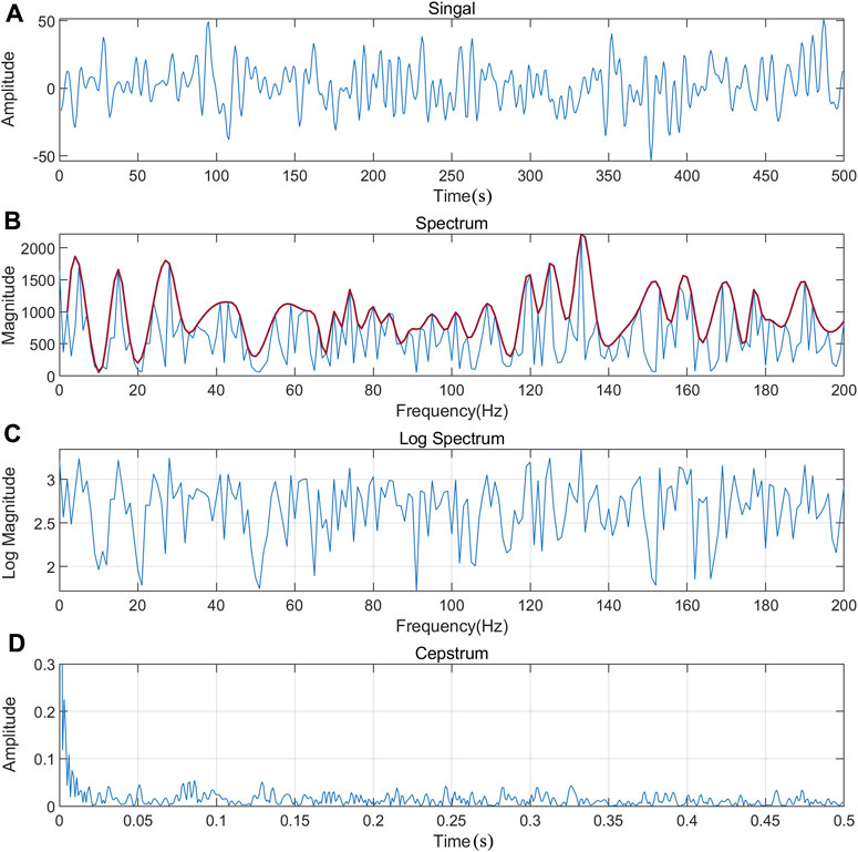
FIGURE 2. Schematic diagram of cepstral analysis. (A) signal and (B) spectrum. The red line is the envelope. (C) Log spectrum and (D) cepstrum.

The mathematical expression is

$\mathit{Z}\left(\mathbf{n}\right)={\mathit{F}}^{-\mathbf{1}}\left[\mathit{log}\left(\mathit{X}\left(\mathit{n}\right)\right)\right],(1)$

where $Z\left(n\right)$ represents the cepstrum and $X\left(n\right)$ is the spectrum. $X\left(n\right)$ after Fourier change in the $X\left(t\right)$ signal can be expressed as

$\mathit{X}\left(\mathit{n}\right)={\int }_{-\mathit{\infty }}^{+\mathit{\infty }}\mathit{x}\left(\mathit{t}\right){\mathit{exp}}^{-\mathit{j}\mathbf{2}\mathit{\pi }\mathit{n}\mathit{t}}\mathit{d}\mathit{t}.(2)$

From the aforementioned equation, it can be seen that the signal retains the amplitude and phase information after the Fourier variation. The cepstrum defined by the Fourier spectrum is further divided into real cepstrum and complex cepstrum.

Then, the signal, through Fourier variation, can be expressed as

$\mathit{X}\left(\mathit{n}\right)=\mathit{A}\left(\mathit{n}\right)\mathit{exp}\left(\mathit{j}\varnothing \left(\mathit{n}\right)\right).(3)$

So there is

$\mathit{ln}\left(\mathit{X}\left(\mathit{n}\right)\right)=\mathit{ln}\left(\mathit{A}\left(\mathit{n}\right)\right)+\mathit{j}\varnothing \left(\mathit{n}\right),(4)$

where $A\left(n\right)$ is the continuous amplitude spectrum of the analysis signal and $\varnothing \left(\mathit{n}\right)$ is the continuous phase spectrum.

When $X\left(n\right)$ retains only the real part, the real cepstrum is defined as

$\mathit{Z}\left(\mathbf{n}\right)={\mathit{F}}^{-\mathbf{1}}\left[\mathit{ln}\left(\mathit{A}\left(\mathit{n}\right)\right)\right].(5)$

It can be found that in the calculation of the cepstrum, real cepstral analysis actually involves zeroing the phase spectrum, which is the “inverse Fourier transform of the logarithmic amplitude spectrum.” Therefore, we need to add back the lost phase when rebuilding the signal after segmental cepstrum; this restoration is crucial for the calculation of the apparent resistivity.

3 Simulation

To demonstrate the effect of the cepstral analysis method, we selected high-quality spectral curves from the measured MT data for easy addition of various types of noise for comparison. First, we verified the impact of different selections of the cepstral cutoff point on the smoothness of the amplitude spectrum. The selected data were processed, and Figures 3A–C depicts the partial amplitude spectrum before and after processing with different cepstral segment positions, with the post-processing amplitude spectrum in blue and the pre-processing amplitude spectrum in yellow. The amplitude spectrum becomes smoother than before the processing by truncating the cepstrum. The change in the truncation position directly affects the smoothness of the amplitude spectrum. However, determining an appropriate truncation point still relies on other parameters. In this study, we have acquired different spectrum smoothness levels and correlations by adjusting the cepstral truncation position. Figure 4 displays the results derived from these two parameters, where the y-axis represents the correlation coefficient of the spectrum before and after processing and the x-axis signifies the roughness of the spectrum. We seek points with a lower degree of roughness on the curve with a high auto-correlation coefficient to serve as truncation points for the processing, as indicated by the range within the red circle in the figure. This provides a basis for the subsequent selection of the cutoff location.

FIGURE 3

FIGURE 3. Comparison chart of amplitude spectrum before and after processing. (A)1/8 truncation: The red line is the original spectrum, and the blue line is the processed spectrum. (B) 2/8 truncation: The red line is the original spectrum, and the blue line is the processed spectrum. (C) 3/8 truncation: The red line is the original spectrum, and the blue line is the processed spectrum.

FIGURE 4

FIGURE 4. Correlation coefficient and roughness curves.

To demonstrate the denoising effect of the cepstral analysis, we add square waves, triangular waves, and impulse noise to the simulation data from 400 to 600 sampling points. We processed the simulation data using the cepstral analysis method. During the procedure, we truncated the latter half of the cepstrum, retaining only the preceding half. By reconstructing the signal, we obtained the processed spectral curves for comparison and further analysis.

Figure 5 shows the comparative analysis of the simulated signal before and after adding triangular wave noise. Figure 5A depicts a segment of the original signal without noise, while Figure 5B portrays the signal with triangular wave-like noise. Figures 5C, D depict the signals processed using the methodology proposed in this study and the EMD method, respectively. Figures 5E–H represent the corresponding spectrum. In Figure 5B, it is evident that the triangular wave-like noise is effectively suppressed using the cepstral analysis and EMD methods. The spectrum on the right further shows that the frequency-domain characteristics of the triangular wave, as shown in Figure 5F, have been substantially eliminated in Figures 5G, H. To further compare the effectiveness of the two methods, we introduce parameters such as signal-to-noise ratio (SNR), mean square error (MSE), and normalized cross-correlation (NCC) (Table 1). The results indicate that the data processed using the cepstral analysis method display a higher SNR and cross-correlation and lower error, underscoring the superior performance of this method. To facilitate the calculation of apparent resistivity and phase, the simulation data were extended to 54,000 points for computation. Figure 6A shows the apparent resistivity curves derived from the noise-added data using two different methods, while Figure 6B shows the phase curves. In Figure 6, the yellow curve represents the apparent resistivity and phase curves obtained through the cepstral method, while the green curve is derived from the EMD method. Upon comparison, it is evident that within the 0.005–0.01 Hz range, the yellow curve is smoother and has fewer errors. Comparing Figures 6C, D it can be seen that the residual map after denoising is closer to 0, effectively removing the noise. This further validates the effectiveness of the methodology presented in this study.

FIGURE 5

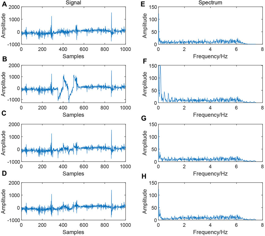
FIGURE 5. Comparison of simulated triangle wave denoising effects. (A) Original signal; (B) signal with triangular wave noise; (C) signal processed using the cepstrum method; (D) signal processed using the EMD method; (E) spectrum of the original signal; (F) spectrum of the signal with triangular wave noise; (G) signal spectrum processed using the cepstrum method; and (H) signal spectrum processed using the EMD method.

TABLE 1

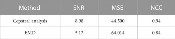
TABLE 1. Signal parameters.

FIGURE 6

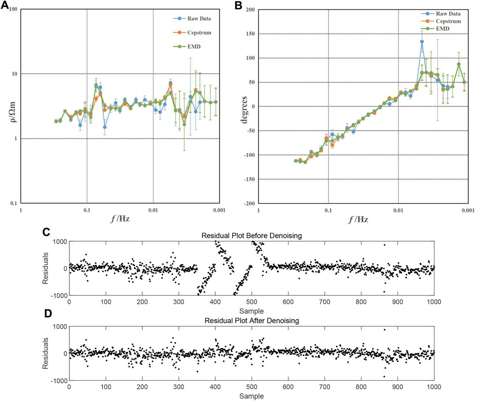
FIGURE 6. Apparent resistivity and phase curves and residual plots. (A) Apparent resistivity curve; (B) phase curve; (C) residual plot before denoising; and (D) residual plot after denoising.

Figure 7 shows the comparison of signal processing before and after adding square wave noise. Figure 7A shows a segment of the original signal without noise, while Figure 6B shows the signal with square wave-like noise. Figures 7C, D demonstrate the signal processed using the cepstral analysis and EMD methods, repectively. Figures 7E–H each depict the corresponding spectrum. From Figure 7B, it can be observed that the square wave-like noise was effectively eliminated using the cepstral analysis and EMD methods. From the spectrum on the right, Figures 6H, 7G show that the spectral characteristics of the square wave in Figure 7F have been essentially eliminated. The results in Table 2 indicate that the data processed using the cepstral analysis method display a higher SNR and NCC and a lower MSE, underscoring the superior performance of this method.

FIGURE 7

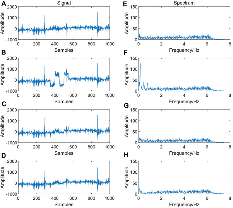
FIGURE 7. Comparison of simulated square wave denoising effects. (A) Original signal; (B) signal with square wave noise; (C) signal processed using the cepstrum method; (D) signal processed using the EMD method; (E) spectrum of the original signal; (F) spectrum of the square wave noise signal; (G) signal spectrum processed using the cepstrum method; and (H) signal spectrum processed using the EMD method.

TABLE 2

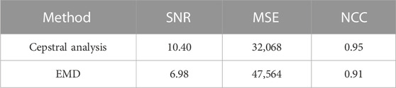
TABLE 2. Signal parameters.

Figure 8A shows the apparent resistivity curves derived from the noise-added data using two different methods, while Figure 8B shows the phase curves. In Figure 8, both methods have effectively suppressed noise, resulting in smoother apparent resistivity curves. However, at the 0.1 Hz mark in Figure 8A, the two increasing frequency points are more prominently addressed using the method proposed in this study, showing a more significant decline. Comparing Figures 8C, D, it can be seen that the residual map after denoising is closer to 0, effectively removing the noise.

FIGURE 8

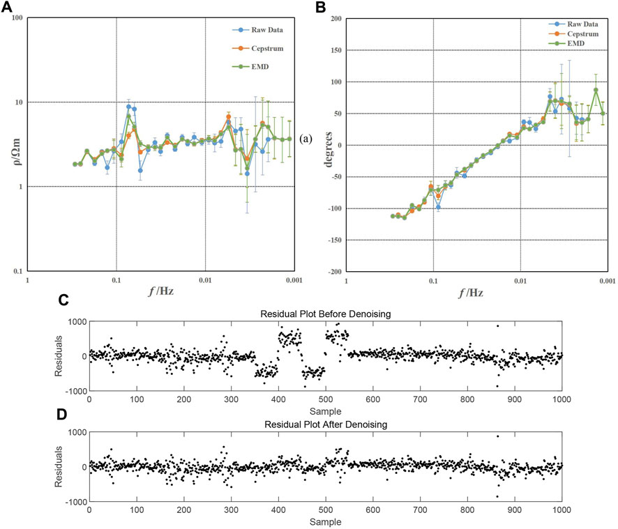
FIGURE 8. Apparent resistivity and phase curves and residual plots. (A) Apparent resistivity curve; (B) phase curve; (C) residual plot before denoising; and (D) residual plot after denoising.

Figure 9 shows the comparison of signal processing before and after adding Gaussian noise. Figure 9A shows a segment of the original signal without noise, while Figure 9B shows the signal with Gaussian noise. Figures 9C, D represent the signals processed using the cepstral analysis and EMD methods, respectively. Figures 9E–H show the corresponding spectrum. By comparing Figure 9B, the Gaussian noise was effectively suppressed using the cepstral analysis and EMD methods. Although we cannot observe the spectral characteristics of the noise being eliminated from the spectrum as in Figures 5, 7, we can still compare the results using parameters such as signal-to-noise ratio, mean square error, and normalized cross-correlation (Table 3). The results indicate that the data processed using the cepstral analysis method display a higher SNR and NCC and a lower MSE, indicating the superior performance of the cepstral analysis method.

FIGURE 9

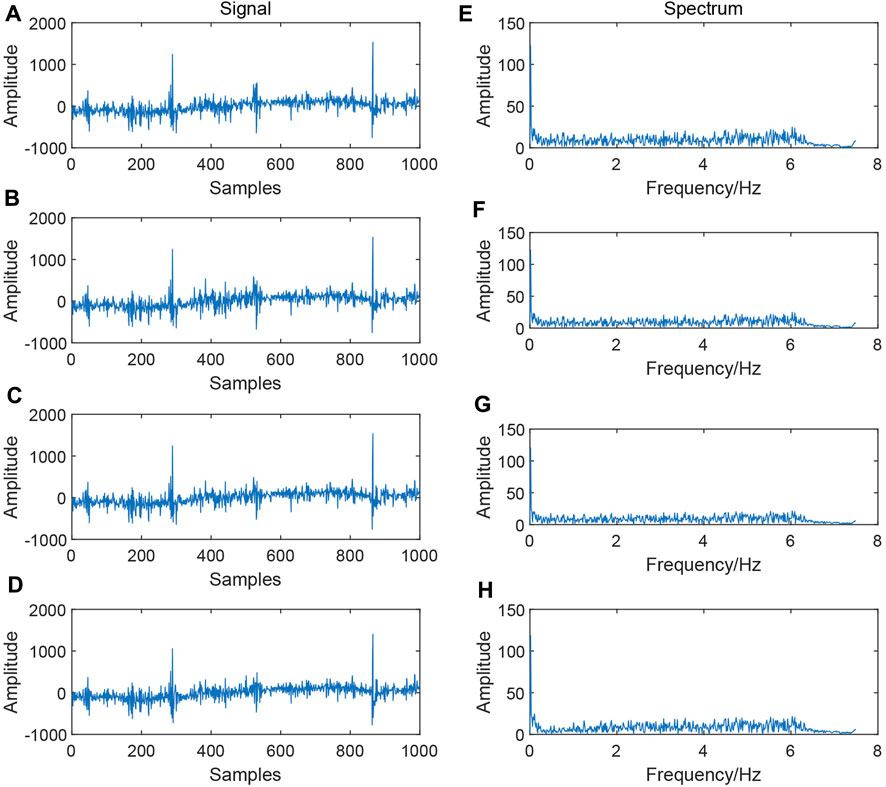
FIGURE 9. Comparison of denoising effects of simulated Gaussian noise. (A) Original signal; (B) signal with Gaussian noise; (C) signal processed using the cepstrum method; (D) signal processed using the EMD method; (E) spectrum of the original signal; (F) spectrum of the Gaussian sound signal; (G) signal spectrum processed using the cepstrum method; and (H) signal spectrum processed using the EMD method.

TABLE 3

TABLE 3. Signal parameters.

Figure 10A shows the apparent resistivity curves derived from the noise-added data using two different methods, while Figure 10B shows the phase curves. In Figure 10, it is challenging to determine whether the noise has been effectively suppressed, both from the waveform and apparent resistivity and phase curves. The residual plots of Figures 10C, D also fail to observe the difference. Compared to the noise of triangular and square waves, the method proposed in this study does not perform well when addressing noise whose waveform and spectrum closely resemble the signal.

FIGURE 10

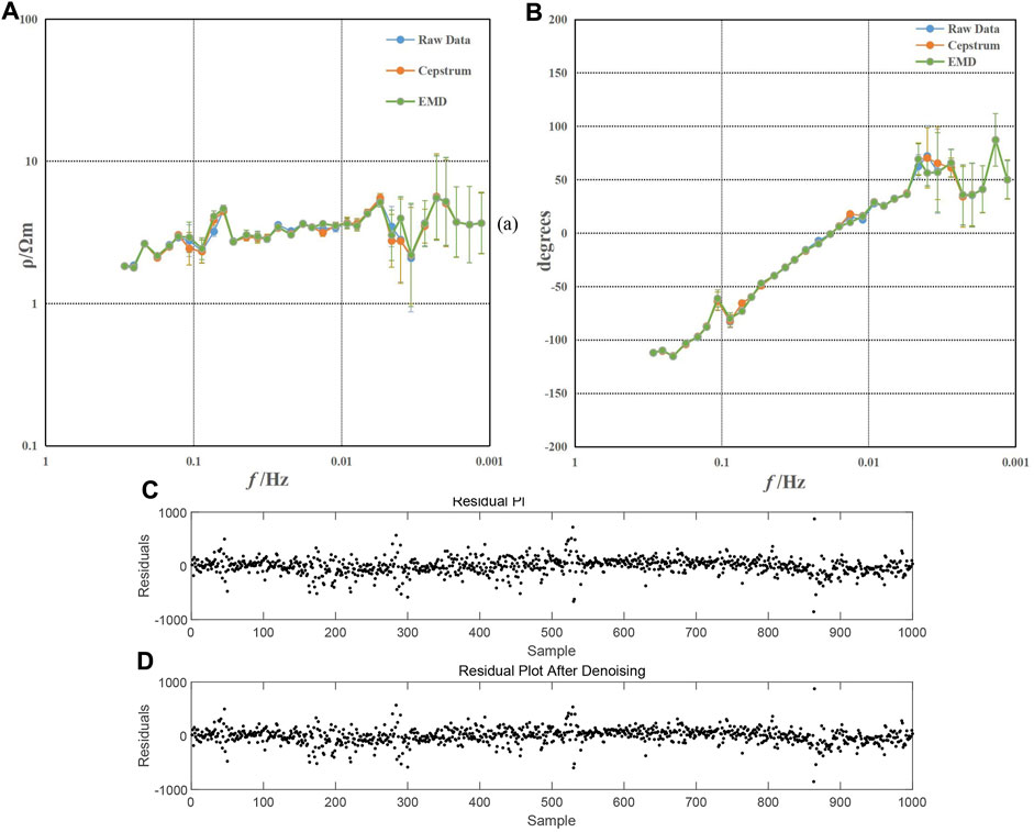
FIGURE 10. Apparent resistivity and phase curves and residual plots. (A) Apparent resistivity curve; (B) phase curve; (C) residual plot before denoising; and (D) Residual plot after denoising.

Based on the analysis and discussion in this section, it becomes evident that the cepstral analysis method proposed in this study outperforms the EMD method in effectively suppressing various types of noise present in the signals. The application of cepstral analysis leads to enhanced smoothness in the spectrum, resulting in improved overall performance.

4 Data processing

To further verify the validity of the proposed method, we selected three measuring points for detailed analysis and discussion. The high-frequency portion of these data is of good quality, while the low-frequency band has noise interference and poor-quality apparent resistivity curves. These characteristics facilitate our subsequent analysis and validation. We used V5-2000 for data acquisition and SSMT-2000 software for apparent resistivity and phase calculations, and we employed the robust method produced by Phoenix Geophysics Limited, Toronto, Canada.

The MT site BH16 is located near the Hepu Industrial Zone, where industrial noise may have an impact on the quality of the signals. The location of the site BH16 is shown in Figure 11. Figures 12A, B depict the apparent resistivity curves in the Rxy and Ryx directions for the site BH16 obtained using three different methods. Given the lower quality of data in the low-frequency range, Figures 12C, D provide a clearer comparison by showcasing the apparent resistivity curves for frequencies less than 0.01 Hz.

FIGURE 11

FIGURE 11. Map showing the location of site B16.

FIGURE 12

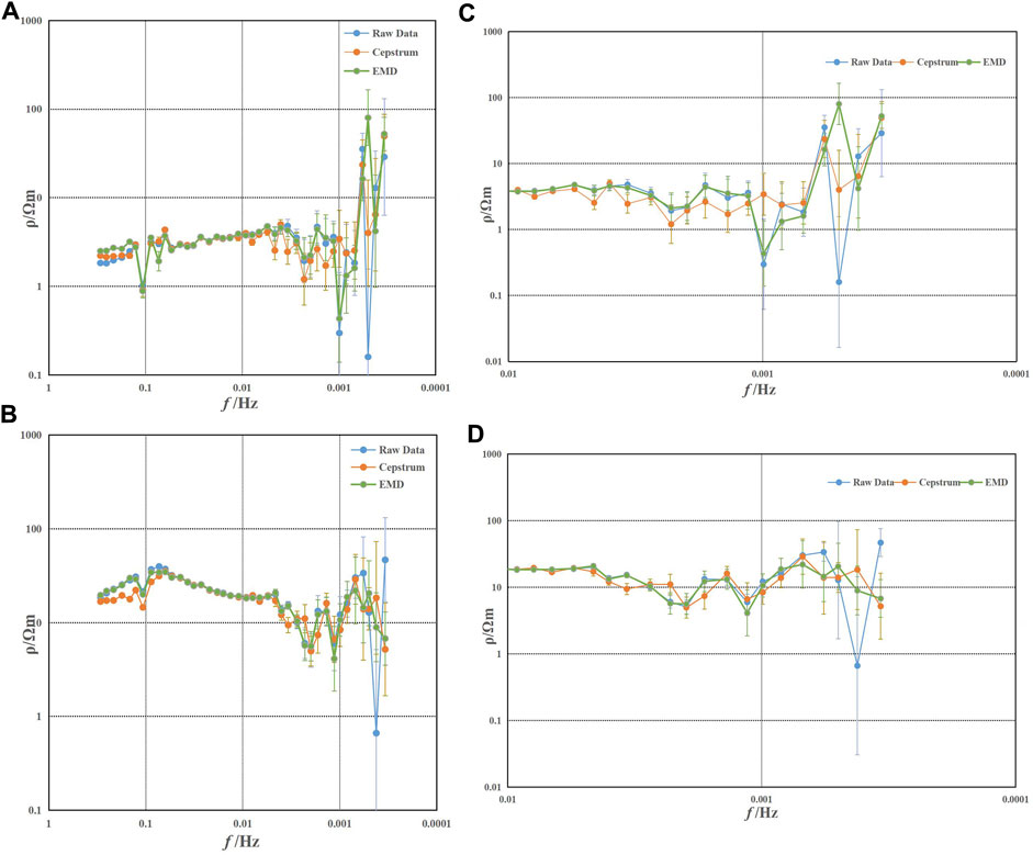
FIGURE 12. Apparent resistivity curve of site BH16. (A) Rxy; (B) Ryx; (C) part of Rxy; and (D) part of Ryx.

Figure 12 shows the apparent resistivity curves of the MT site BH16 obtained from the original data, the EMD method, and the proposed method. Figures 12A, C represent the Rxy direction, while Figures 12B, D represent the Ryx direction. The blue curve has poor continuity and smoothing of apparent resistivity, which represents the original data. Within the frequency range of 0.1–0.008 Hz, the apparent resistivity curve appears relatively smooth with a small range of errors. However, in the frequency range of 0.008–0.0005 Hz, the data of approximately 12 frequency points are completely distorted. At approximately 0.0005 Hz, the apparent resistivity curve shows significant fluctuations with large errors. In Figure 12C, the apparent resistivity in the Rxy direction reaches a minimum value close to 0.1 Ω·m and a maximum value close to 60 Ω·m. In Figure 12D, the apparent resistivity in the Ryx direction reaches a minimum value close to 0.9 Ω·m and a maximum value close to 70 Ω·m. Because of noise interference, the time–frequency characteristics cannot reflect the true typical features of the subsurface.

The yellow curve in Figure 12 represents the apparent resistivity curve of the MT site BH16 processed using the proposed cepstral method. The green curve demonstrates the process of decomposing the original signal into various scale components using the EMD method, extracting the approximate single component of each intrinsic mode function from high to low frequencies, and then reconstructing the signal by removing the high-frequency IMF component. Comparing the three curves in the low-frequency range, it can be observed that both methods effectively suppress noise interference to some extent. However, the proposed method obtains more significant results with relatively smoother apparent resistivity curves. Particularly in the Rxy direction, the sudden frequency drops near 0.001 Hz and 0.0008 Hz tend to approach normal levels, and the errors in the low-frequency range are reduced, resulting in relatively stable numerical values.

Figures 14, 15 show data obtained from Xiwuqi, Inner Mongolia, in close proximity to Gaorihan Town, with surrounding agricultural households and frequent livestock passing through, generating anthropogenic noise that may impact signal quality. The location of the point is shown in Figure 13.

FIGURE 13

FIGURE 13. Map showing the locations of sites 025 and 086.

Figures 14A, B depict the apparent resistivity curves in the Rxy and Ryx directions for the site MT086, obtained using three different methods. In the high-frequency range, the signal strength is relatively weak. The proposed method in this paper tends to de-truncate the high-frequency noise and retain the low-frequency trend when dealing with the cepstrum of the signal. Therefore, it is easy to increase the errors in the high-frequency band if it is processed too much, so in case of poor quality of this band, manual adjustments are usually needed. For the low-frequency band, the cepstrum analysis method is used. Figures 14C, D provide a clearer comparison by showcasing the apparent resistivity curves for frequencies less than 0.01 Hz.

FIGURE 14

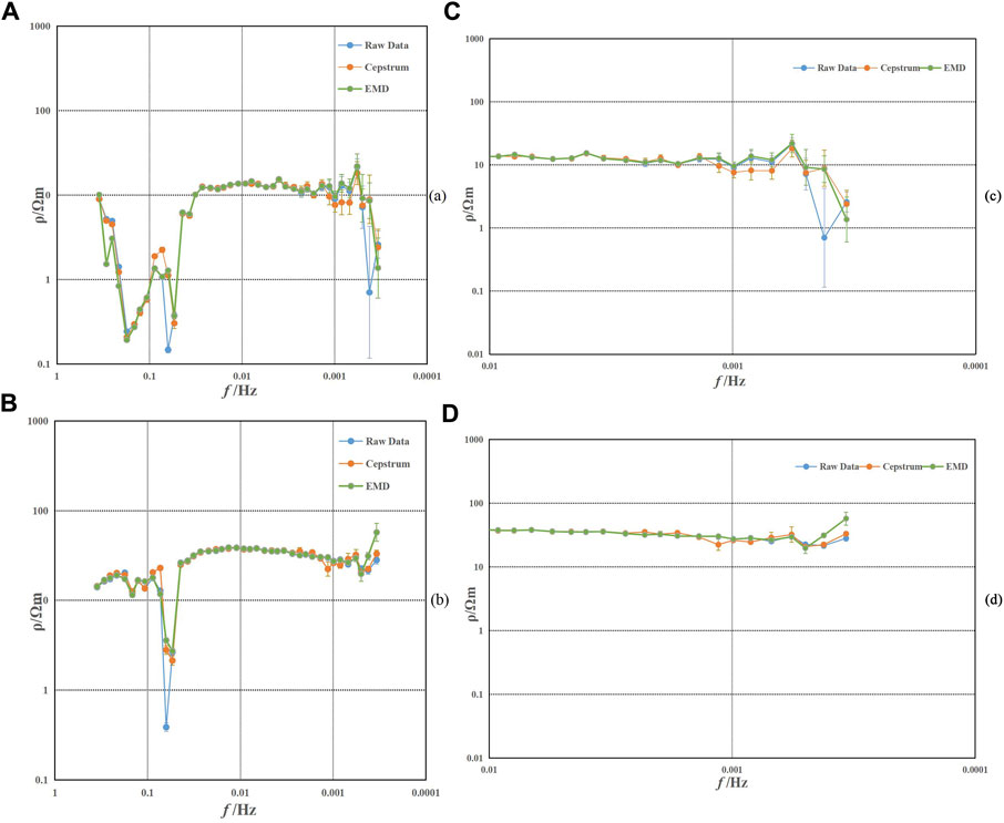
FIGURE 14. Apparent resistivity curve of site MT086. (A) Rxy; (B) Ryx; (C) part of Rxy; and (D) part of Ryx.

Figure 14 shows the apparent resistivity curves of the MT site MT086 obtained from the original data, processed using EMD, and processed using the cepstral method. Figures 14A, C represent the Rxy direction, while Figures 14B, D represent the Ryx direction. In Figure 14C, the overall smoothness of the blue apparent resistivity curve is poor, which represents the original data, and there are significant variations in the low-frequency range. Within the frequency range of 0.08 Hz–0.001 Hz, the curve appears smooth with small errors. However, in the frequency range of 0.001 Hz–0.0005 Hz, the data from approximately four frequency points are completely distorted. At approximately 0.0008 Hz, the resistivity rapidly drops to approximately 0.9 Ω·m, followed by significant fluctuations in the resistivity curve. At 0.0008 Hz, the resistivity sharply decreases to 0.1 Ω·m. Due to noise interference, the time–frequency characteristics of this MT site fail to reflect the true typical subsurface features.

The yellow curve in Figure 14 represents the apparent resistivity curve obtained using the cepstral analysis method, while the green curve represents the apparent resistivity curve obtained using the EMD method. In the low-frequency range, the EMD method does not obtain significant improvement around the distorted frequency point near 0.0006 Hz, but it reduces the magnitude of the drop to some extent (Figure 14C). However, in the Ryx direction, the EMD method shows inferior results (Figure 14D). In contrast, the proposed method in this study demonstrates more significant effects, thus successfully suppressing noise interference in the low-frequency range (approximately 0.0006 Hz). Overall, the resulting apparent resistivity curve appears smooth, with a reduction in error values for several high fluctuation frequency points, resulting in relatively stable numerical values.

Figures 15A, B depict the apparent resistivity curves in the Rxy and Ryx directions for the site MT025 obtained using three different methods. In the high-frequency range, the signal strength is relatively weak, and adjustments are typically made manually. Figures 15C, D provide a clearer comparison by showcasing the apparent resistivity curves for frequencies less than 0.01 Hz.

FIGURE 15

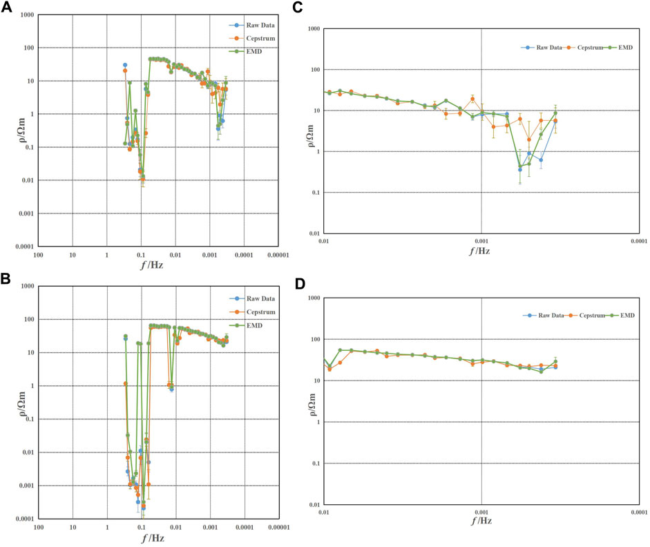
FIGURE 15. Apparent resistivity curve of site MT025. (A) Rxy; (B) Ryx; (C) part of Rxy; and (D) part of Ryx.

Figure 15 shows the apparent resistivity curves of the MT site MT025 obtained from the original data and processed using the EMD cepstral methods. Figures 15A, C represent the Rxy direction, while Figures 15B, D represent the Ryx direction. In Figure 15C, the overall smoothness of the blue apparent resistivity curve is poor, which represents the original data, and the overall continuity of the resistivity curve shape is also poor. There are significant variations in resistivity in the low-frequency range. The resistivity curve appears relatively smooth within the frequency range of 0.01–0.001 Hz. However, in the frequency range of 0.001–0.0005 Hz, data from approximately four frequency points are completely distorted. At approximately 0.0008 Hz, there is a rapid drop followed by an increase at approximately 0.0005 Hz. Because of noise interference, the time–frequency characteristics of this MT site fail to reflect the true typical subsurface features.

The yellow curve in Figure 15 represents the apparent resistivity curve obtained using the cepstral analysis method. The green curve represents the apparent resistivity curve obtained using the EMD method. Comparing the low-frequency range in Figure 15C, the EMD method shows little improvement at a few distorted frequency points. In contrast, the proposed method in this study shows more significant effects in the low-frequency range. It improves all four distorted frequency points at approximately 0.0006 Hz, although there is a slight performance decrease in the front part of the curve. Overall, the resulting apparent resistivity curve appears relatively smooth, with a reduction in error values at several significant fluctuation frequency points, resulting in relatively stable numerical values.

5 Conclusion and discussion

To apply cepstral analysis to the processing of MT data, this study selected three sets of field-collected MT data. The process of cepstral analysis involves homomorphic deconvolution of the data, transforming the multiplicative signal into an additive signal, and then separating the noise through filtering in the cepstral domain. The key to denoising is the selection of the truncation position and the choice of filtering. Choosing a truncation position that is too large may result in the loss of useful information, while selecting a position that is too small may not effectively suppress the noise. The selection of an appropriate filter depends on the characteristics of the data. The results of this study demonstrate that, compared to traditional methods such as robust and EMD, the proposed method in this study shows better performance in handling MT data. The processed apparent resistivity curves exhibit smoother and more continuous characteristics, particularly in the low-frequency range, where the quality of the curves is significantly improved with a substantial reduction in errors. Furthermore, this method has been introduced for the first time in the processing of MT data, offering a novel approach with clear physical significance and a simple pipeline, providing a new direction for future MT data processing. However, it also has limitations because the spectral envelope of the signal approaches that of the noise, which is not effective in successfully suppressing the noise. This method calculates the cepstrum based on the amplitude spectrum of the data, and the quality of the phase curve has not been significantly improved, leaving room for further improvement. The determination of the optimal truncation position still requires iterative experiments. Therefore, future research can explore the integration of adaptive algorithms to dynamically select the optimal truncation position based on the quality of the apparent resistivity and amplitude spectrum curves, further enhancing the data quality. Nonetheless, additional experimental validation and verification of this theory are required. It is crucial to process and invert a larger dataset of MT data to gain a more comprehensive understanding of the MT profiles and underground structures, which will be the focus of future work.

Data availability statement

The data analyzed in this study are subjected to the following licenses/restrictions: Group project. Requests to access these datasets should be directed to QZ, 292800073@qq.com.

Author contributions

All authors listed have made a substantial, direct, and intellectual contribution to the work and approved it for publication.

Conflict of interest

The authors declare that the research was conducted in the absence of any commercial or financial relationships that could be construed as a potential conflict of interest.

Publisher’s note

All claims expressed in this article are solely those of the authors and do not necessarily represent those of their affiliated organizations, or those of the publisher, the editors, and the reviewers. Any product that may be evaluated in this article, or claim that may be made by its manufacturer, is not guaranteed or endorsed by the publisher.

References

Bogert, B. P. (1963). “The quefrency alanysis of time series for echoes: cepstrum, pseudoautocovariance, cross-cepstrum and saphe cracking,” in Proc. Symposium time series analysis (Wuhan, China: Scientific Research Publishing), 209–243.

Google Scholar

Cagniard, L. (1953). Basic theory of the magneto-telluric method of geophysical prospecting. Geophysics 18, 605–635. doi:10.1190/1.1437915

CrossRef Full Text | Google Scholar

Cai, J.-H., Tang, J.-T., Hua, X.-R., and Gong, Y.-R. (2009). An analysis method for magnetotelluric data based on the Hilbert–Huang Transform. Explor. Geophys. 40, 197–205. doi:10.1071/eg08124

CrossRef Full Text | Google Scholar

Cai, J. (2014). A combinatorial filtering method for magnetotelluric time-series based on Hilbert–Huang transform. Explor. Geophys. 45, 63–73. doi:10.1071/eg13012

CrossRef Full Text | Google Scholar

Carbonari, R., D'Auria, L., Rosa Di Maio, , and Petrillo, Z. (2017). Denoising of magnetotelluric signals by polarization analysis in the discrete wavelet domain. Comput. Geosciences 100, 135–141. doi:10.1016/j.cageo.2016.12.011

CrossRef Full Text | Google Scholar

Chave, A. D., Thomson, D. J., and Ander, M. E. (1987). On the robust estimation of power spectra, coherences, and transfer functions. J. Geophys. Res. Solid Earth 92, 633–648. doi:10.1029/jb092ib01p00633

CrossRef Full Text | Google Scholar

Chave, A. D., and Thomson, D. J. (1989). Some comments on magnetotelluric response function estimation. J. Geophys. Res. Solid Earth 94, 14215–14225. doi:10.1029/jb094ib10p14215

CrossRef Full Text | Google Scholar

Chave, A. D. (2017). Estimation of the magnetotelluric response function: the path from robust estimation to a stable maximum likelihood estimator. Surv. Geophys. 38, 837–867. doi:10.1007/s10712-017-9422-6

CrossRef Full Text | Google Scholar

Choi, Y.-C., and Kim, Y.-H. (2007). Fault detection in a ball bearing system using minimum variance cepstrum. Meas. Sci. Technol. 18, 1433–1440. doi:10.1088/0957-0233/18/5/031

CrossRef Full Text | Google Scholar

Constable, S. C., Parker, R. L., and Constable, C. G. (1987). Occam’s inversion: a practical algorithm for generating smooth models from electromagnetic sounding data. Geophysics 52, 289–300. doi:10.1190/1.1442303

CrossRef Full Text | Google Scholar

Dong, S., Li, T., Chen, X., Wei, W., Gao, R., Lv, Q., et al. (2012). Progress of deep exploration in mainland China. Chin. J. Geophys. 55, 3884–3901. doi:10.6038/j.issn.0001-5733.2012.12.002

CrossRef Full Text | Google Scholar

Egbert, G. D., and Booker, J. R. (1986). Robust estimation of geomagnetic transfer functions. Geophys. J. Int. 87, 173–194. doi:10.1111/j.1365-246x.1986.tb04552.x

CrossRef Full Text | Google Scholar

Gamble, T. D., Goubau, W. M., and Clarke, J. (1979). Magnetotellurics with a remote magnetic reference. Geophysics 44, 53–68. doi:10.1190/1.1440923

CrossRef Full Text | Google Scholar

Gangi, A. F., and Shapiro, J. N. (1979). A propagating algorithm for determining nth-order polynomial, least-squares fits; discussion and reply. Geophysics 44, 1588–1591.

CrossRef Full Text | Google Scholar

Garcia, X., and Jones, A. G. (2008). Robust processing of magnetotelluric data in the AMT dead band using the continuous wavelet transform. Geophysics 73, F223–F234. doi:10.1190/1.2987375

CrossRef Full Text | Google Scholar

Jing, J.-En, Wei, W.-Bo, Chen, H.-Y., and Jin, S. (2012). Magnetotelluric sounding data processing based on generalized S transformation. Chin. J. Geophys. 55, 4015–4022.

Google Scholar

Kim, G.-S., Cho, G.-R., Jong-Nam, K., Yong-Chol, P., Sung-Hyon, Ri, and Hu, X.-Y. (2018). 'Constrained smoothness optimization of bootstrapped transfer functions for handling noisy MT data. J. Appl. Geophys. 155, 226–231. doi:10.1016/j.jappgeo.2018.05.018

CrossRef Full Text | Google Scholar

Li, H., Zheng, H., and Tang, L. (2006a). Application of order cepstrum to bearing fault diagnosis. J. Data Acquis. Process. 21, 454–458.

Google Scholar

Li, X. (2012). Research on feature extraction and classification of ship noise and whale sound. Harbin, China: Harbin Engineering University.

Google Scholar

Li, Y., Sun, X., and Zhou, T. (2006b). Research on digital audio watermark bsaed on complex cepstrum transform. Comput. Eng. 32, 145–147.

Google Scholar

Manoj, C., and Nagarajan, N. (2003). The application of artificial neural networks to magnetotelluric time-series analysis. Geophys. J. Int. 153, 409–423. doi:10.1046/j.1365-246x.2003.01902.x

CrossRef Full Text | Google Scholar

Randall, R. B., and Sawalhi, N. (2011). A new method for separating discrete components from a signal. Sound Vib. 45, 6.

Google Scholar

Ritter, O., Junge, A., and Dawes, G. J. K. (1998). New equipment and processing for magnetotelluric remote reference observations. Geophys. J. Int. 132, 535–548. doi:10.1046/j.1365-246x.1998.00440.x

CrossRef Full Text | Google Scholar

Tang, J.-T., Jin, Li, Xiao, X., Zhang, L.-C., and Qing-Tian, L. V. (2012). Mathematical morphology filtering and noise suppression of magnetotelluric sounding data. Chin. J. Geophys. 55, 1784–1793.

Google Scholar

Tikhonov, A. N. (1950). On determining electrical characteristics of the deep layers of the Earth's crust. Dokl. Akad. Nauk. SSSR, 295–297.

Google Scholar

Trad, D. O., and Jandyr, M. (2000). Wavelet filtering of magnetotelluric data. Geophysics 65, 482–491. doi:10.1190/1.1444742

CrossRef Full Text | Google Scholar

Wang, J.-ying (2004b). Discussion on the non-minimum phase of magnetotelluric signals. Prog. Geophys. | Prog Geophys 19, 216–221.

Google Scholar

Wang, S., and Wang, J. (2004a). Application of higher-order statistics in magnetotelluric data processing. Chin. J. Geophys. 47, 1046–1053. doi:10.1002/cjg2.584

CrossRef Full Text | Google Scholar

Wei, F., and Li, M. (2003). Cepstrum analysis of source character. Acta Seismol. Sin. 25, 47–54.

Google Scholar

Wei, W.-Bo (2002). New advance and prospect of magnetotelluric sounding (MT) in China. Prog. Geophys. | Prog Geophys 17, 245–254.

Google Scholar

Weidelt, P. (1972). 'The inverse problem of geomagnetic induction. Z. Geophys. 38, 257–289.

Google Scholar

Xie, T., and Zheng, X. (2016). 'Seismic facies analysis based on linear prediction cepstrum coefficients. Chin. J. Geophys. 59, 4266–4277.

Google Scholar

Zeng, Z., Li, Y., and Liu, X. (2011). Study on feature extraction of ship radiated noise based on higher order spectrum and cepstrum. Comput. Simul. 28, 5–9.

Google Scholar