Joint denoising method of seismic velocity signal and acceleration signals based on independent component analysis

The signal-to-noise ratio (SNR) of seismic data is the key to seismic data processing, and it also directly affects interpretation of seismic data results. The conventional denoising method, independent variable analysis, uses adjacent traces for processing. However, this method has problems, such as the destruction of effective signals. The widespread use of velocity and acceleration geophones in seismic exploration makes it possible to obtain different types of signals from the same geological target, which is fundamental to the joint denoising of these two types of signals. In this study, we propose a joint denoising method using seismic velocity and acceleration signals. This method selects the same trace of velocity and acceleration signal for Independent Component Analysis (ICA) to obtain the independent initial effective signal and separation noise. Subsequently, the obtained effective signal and noise are used as the prior information for a Kalman filter, and the final joint denoising results are obtained. This method combines the advantages of low-frequency seismic velocity signals and high-frequency and high-resolution acceleration signals. Simultaneously, this method overcomes the problem of inconsistent stratigraphic reflection caused by the large spacing between adjacent traces, and improves the SNR of the seismic data. In a model data test and in field data from a work area in the Shengli Oilfield, the method increases the dominate frequency of the signal from 20 to 40 Hz. The time resolution was increased from 8.5 to 6.8 ms. The test results showed that the joint denoising method based on seismic velocity and acceleration signals can better improve the dominate frequency and time resolution of actual seismic data.

1 Introduction

With the development of exploration technology, exploration targets have changed from large, thick, and high porosity reservoirs to small, thin, low porosity reservoirs, and from structural reservoirs to stratigraphic, lithological, and other complex reservoirs. Requirements for exploration resolution and accuracy are increasing. Seismic data denoising is a key step in seismic data processing and affects subsequent data interpretation (Han and Van, 2013). Conventional suppression methods for random noise in seismic data are mainly divided into space domain and transform domain methods (Necati, 1986; Joachim, 1997). Noise suppression methods in the space domain can be divided into median filtering (Wang et al., 2012), diffusion filtering (Perona and Malik, 1990), etc.,; The methods in transform domain noise suppression can be divided into frequency domain denoising (Necati, 1986), wavelet transform denoising (Morlet et al., 1982), meander transform denoising (Cao et al., 2015), and empirical mode decomposition-based denoising methods (Mirko and Maiza, 2009). Median filter denoising can easily destroy the continuity of events and lose detail (Chen et al., 2019). Diffusion filtering lacks the use of nonlocal information, which may damage some effective signals (Wang et al., 2021). Although frequency-domain denoising is one of the most commonly-used denoising methods, it cannot suppress noise in the frequency range that coincides with the effective signal (Sergio and Tad, 1988). Wavelet transform denoising can only perform signal transformation in a single direction, and cannot adapt to signals with multi-directional changes (Spanias et al., 1991). Curved transform denoising is a derivative of wavelet transform denoising, which overcomes the above disadvantages; however, it has other problems, such as slow computing efficiency (Cao et al., 2012). The denoising method based on empirical mode decomposition has the problems of low accuracy or instability in the decomposition process due to boundary effects, and mode aliasing occurs during the decomposition process (Damaševičius et al., 2017). In addition, these methods only use one type of data for processing, and so cannot take into consideration the advantages of multiple signals from different geophones.

Velocity and acceleration geophones are widely used in seismic exploration to satisfy the requirements of high-precision exploration (Nicolas and Jérôme, 2017). By comparing the frequency characteristics and waveforms of the velocity and acceleration signals, Hons et al. (2007; 2008) proposed that the two signals were similar after mathematical conversion, and that there was only a slight difference in the main wave. However, the acceleration signal has a wider frequency band than the velocity signal, which improves seismic resolution (Denis, 2004; Zhang et al., 2020). In addition, some researchers have shown that the acceleration signal has little waveform distortion, high signal-to-noise ratio (SNR), and fidelity (Lansley et al., 2008; Liu et al., 2012; Bai et al., 2014). By comparing the frequency band information of different signals in the same domain, Ren (2018) proposed that the velocity signal has more information in the low-frequency region than the acceleration signal, and the acceleration signal has more information in the high-frequency region than the velocity signal. Wei (2018) pointed out that in the filed seismic data, the SNR of the velocity signal is higher than the acceleration signal. But the acceleration signal has a higher dominate frequency. Although in theory the velocity and acceleration signals can be consistent after mathematical transformation, different types of geophones have different advantages in actual acquisition. Therefore, the velocity and acceleration signals can be combined for denoising, and the respective advantages of the two signals can be retained.

Using the observed signal to separate the effective signal and noise is a problem of blind source separation. Blind source separation problem is that only the observed mixed signal is used to recover the source signal when both the source signal and transmission channel are unknown During signal transmission (Zhang et al., 2022). Independent component analysis (ICA) is one of the most effective and widely-used methods for solving this problem. Based on the adjacent seismic traces approximation theory, Meng and Su (Meng et al., 2021) used ICA to separate noise and effective signals to improve the resolution of seismic data. At the same time, ICA requires that the number of observed signals be greater than or equal to the number of source signals. For consistency, conventional ICA approximates the reflection coefficients of adjacent seismic traces. However, when the spacing between adjacent traces is too large, or when there are special geological structures between adjacent traces, there are large differences between the formation reflection coefficients of adjacent seismic traces. Nonetheless, when the formation reflection coefficients of the same trace of the velocity and acceleration signals are consistent, and there is no such problem. Owing to the consistency of the reflection coefficient, the effective signals of the velocity and acceleration signals can be consistent after mathematical transformation, but different types of signals have different noise signals due to different acquisitions. Therefore, the velocity and acceleration signals of the same trace can be considered to have certain differences that satisfy the requirements of ICA.

In this paper, we propose a joint denoising method based on seismic velocity and acceleration signals. First, based on the mathematical relationship between the speed and acceleration signals, ICA is used to obtain approximately independent effective and noise signals. Second, the effective and noise signals obtained by ICA are taken as the prior information for the Kalman filter, which provides the Kalman estimation components more comprehensive prior information. Denoising data can then be obtained after joint processing.

This method is based on the theoretical relationship between seismic velocity and acceleration signals, and uses ICA and Kalman filter for denoising. At the same time, this method takes into account the advantages of velocity and acceleration signals, solves the problem of the inconsistency of adjacent traces data, and thus improves the resolution of seismic signal and is suitable for further application.

2 Materials and methods

2.1 Independent component analysis

As an independent source signal separation method, ICA is one of the most effective and widely-used methods for solving the problem of blind source separation (Saruwatari et al., 2006). The ICA method can realize the separation of effective seismic signal and random noise according to their statistical characteristics (Liu et al., 2007). ICA is a method for determining a set of non-orthogonal coordinate systems in multidimensional data, and obtaining another set of statistically independent data in the original multidimensional data through the projection of coordinates. This method requires that the number of observed signals be greater than the number of source signals, and that the source signals are independent of each other and follow a non-Gaussian distribution (Qin et al., 2018). In seismic data, the required effective signal and noise are independent of each other. In addition, a seismic wavelet can be considered as a non-Gaussian distribution. Therefore, seismic signals meet the preconditions of the ICA method, which can be used to separate seismic signals from noise.

The ICA requirement that the number of observed signals be greater than the number of source signals is generally based on multiple observations of data from the same or similar channels. The actual seismic data have many seismic traces, and each seismic data point can be regarded as an independent one-dimensional signal. If each seismic trace is processed separately, the number of observed data points is less than the number of source signals. The data obtained from separate observations of the velocity and acceleration signals of the same seismic trace satisfy the preconditions of ICA.

In the mathematical model of ICA it is assumed that there are m source signals $\mathit{S}={\left({\mathit{s}}_{\mathbf{1}},{\mathit{s}}_{\mathbf{2}},\dots ,{\mathit{s}}_{\mathit{m}}\right)}^{\mathit{T}}$, n mixed signals $\mathit{X}={\left({\mathit{x}}_{\mathbf{1}},{\mathit{x}}_{\mathbf{2}},\dots ,{\mathit{x}}_{\mathit{n}}\right)}^{\mathit{T}}$. Mixed signals composed of mixed source signals are obtained after passing through an unknown system A, and then m estimated source signals $\mathit{Y}={\left({\mathit{y}}_{\mathbf{1}},{\mathit{y}}_{\mathbf{2}},\dots ,{\mathit{y}}_{\mathit{m}}\right)}^{\mathit{T}}$ are obtained by blind separation system B. When the estimated source signal Y is infinitely close to the real source signal S, source signal S (which cannot be obtained by direct observation) is obtained. Figure 1 shows the system model of ICA.

FIGURE 1

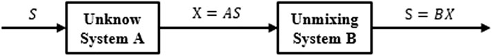
FIGURE 1. Independent component analysis model.

The denoising method based on ICA can be described as follows:

Assume there are m source signals $\mathit{S}={\left({\mathit{s}}_{\mathbf{1}},{\mathit{s}}_{\mathbf{2}},\dots ,{\mathit{s}}_{\mathit{m}}\right)}^{\mathit{T}}$, and n observed signals $\mathit{X}={\left({\mathit{x}}_{\mathbf{1}},{\mathit{x}}_{\mathbf{2}},\dots ,{\mathit{x}}_{\mathit{n}}\right)}^{\mathit{T}}$, which can be expressed as

${\mathit{x}}_{\mathit{i}}={\mathit{a}}_{\mathit{i}\mathbf{1}}{\mathit{s}}_{\mathbf{1}}+{\mathit{a}}_{\mathit{i}\mathbf{2}}{\mathit{s}}_{\mathbf{2}}+\dots +{\mathit{a}}_{\mathit{i}\mathit{m}}{\mathit{s}}_{\mathit{m}}(1)$

where $\mathit{i}=\mathbf{1,2},\dots ,\mathit{n}$.

Rewrite Eq. 1 into vector form,

$\mathit{X}=\mathit{A}\mathit{S}(2)$

where A is the mixed matrix of the unknown system, which can be expressed as

$\mathit{A}=\left(\begin{array}{ccc}{\mathit{a}}_{\mathbf{11}}& \dots & {\mathit{a}}_{\mathbf{1}\mathit{j}}\\ ⋮& \ddots & ⋮\\ {\mathit{a}}_{\mathit{i}\mathbf{1}}& \dots & {\mathit{a}}_{\mathit{i}\mathit{j}}\end{array}\right)(3)$

where ${\mathit{a}}_{\mathit{i}\mathit{j}}$ represents the influencing factor of the jth source signal in the ith observed signal, i=1,2... n, j=1,2... m.

Equation. 2 represents the standard ICA model. In actual seismic data, the observed signal X is known, whereas the source signal S and mixed matrix A are unknown. Assuming that the mixture matrix A is invertible, Eq. 2 can be written as

$\mathit{S}=\mathit{B}\mathit{X}(4)$

where B is the inverse of the mixed matrix A.

The core function of ICA is to obtain the above Eq. 4, obtain matrix B, and then realize the separation of the observed signal X, and finally obtain different source signals S.

Prior to ICA, the data need to be zero-centered and whitened. The purpose of zero-centering is to make the mean value of each data observation zero, and simplify the ICA algorithm. The purpose of whitening is to remove the correlation between observed signals, so that the algorithm convergence speed is faster and the algorithm is more stable during ICA.

Zero-centering can be expressed as:

${\mathit{X}}_{\mathit{i},\mathit{j}}={\mathit{X}}_{\mathit{i},\mathit{j}}-{\mathit{X}\mathit{m}}_{\mathit{j}}(5)$

where X is the observed data, ${\mathit{X}}_{\mathit{i},\mathit{j}}$ is the i-row data of the jth channel, and ${\mathit{X}\mathit{m}}_{\mathit{j}}$ is the mean value of the observed data of the jth channel.

Whitening can be expressed as:

$\mathit{X}\mathit{w}={\mathit{D}}^{-\mathbf{1}}{\mathit{I}}^{-\mathbf{1}}\mathit{X}(6)$

where $\mathit{X}\mathit{w}$ is the data after whitening, D is the eigenvalue of the covariance data of data X after zero-centering, and I is the identity matrix.

When calculating the separation matrix B, negative entropy was adopted in this study as a measure of non-Gaussian signal. The iterative equation of the ICA algorithm can be expressed as (Hajsadeghi et al., 2020):

${\mathit{b}}_{\mathit{k}+\mathbf{1}}=\mathit{E}\left\{{\mathit{X}}_{\mathit{w}}{\mathit{G}}^{\prime }\left({\mathit{b}}_{\mathit{k}}^{\mathit{T}}{\mathit{X}}_{\mathit{w}}\right)\right\}-\mathit{E}\left\{{\mathit{G}}^{″}\left({\mathit{b}}_{\mathit{k}}^{\mathit{T}}{\mathit{X}}_{\mathit{w}}\right)\right\}{\mathit{b}}_{\mathit{k}}(7)$

where b is the row vector of separation matrix B, ${\mathit{X}}_{\mathit{w}}$ is the observed data after whitening, and G can be selected in different expressions according to the type of signal. This method selects (Hajsadeghi et al., 2020):

$\left\{\begin{array}{c}{\mathit{G}}^{\prime }\left({\mathit{X}}_{\mathit{w}}\right)=-\frac{\mathbf{1}}{\mathit{a}}\mathit{exp}\left(-\mathit{a}{\mathit{X}}_{\mathit{w}}^{\mathbf{2}}/\mathbf{2}\right)\\ {\mathit{G}}^{″}\left({\mathit{X}}_{\mathit{w}}\right)={\mathit{X}}_{\mathit{w}}\mathit{exp}\left(-\mathit{a}{\mathit{X}}_{\mathit{w}}^{\mathbf{2}}/\mathbf{2}\right)\end{array}\right.(8)$

where ${\mathit{X}}_{\mathit{w}}$ is the observed data after whitening, the value of a is about 1, ${\mathit{G}}^{\prime }$ represents the first derivative of G, ${\mathit{G}}^{″}$ represents the second derivative of G.

The final separation matrix B can be obtained after satisfying the iteration termination condition. Using the separation matrix B, the observed signal X can be reconstructed to obtain the source signal S.

2.2 Kalman filter method

Although the ICA method has the advantages of fast convergence speed, ease of use, simple calculation, and small memory requirement, the order of the output vectors and the amplitude of the output signal are uncertain. The Kalman filter method has the problem of uncertainty of prior information. The decomposition components obtained by ICA of seismic records can provide Kalman filter components with more comprehensive prior information. Therefore, the Kalman filter method is used to denoise the acceleration and the original acceleration signals by using the information obtained from the ICA as the prior information.

The mathematical model of the Kalman filter method is divided into two types of equations: the state equation and observation equation. These two equations are used to describe the system. The state equation can be written as (Ott and Meder, 1972):

${\mathit{X}}_{\mathit{k}}={\mathit{\Phi }}_{\mathit{k}}{\mathit{X}}_{\mathit{k}-\mathbf{1}}+{\mathit{W}}_{\mathit{k}}(9)$

where ${\mathit{X}}_{\mathit{k}}$ is the n-dimensional column vector and is the state of the system at time k. ${\mathit{\Phi }}_{\mathit{k}}$ is a square matrix of order n × n, which is the state transition square matrix of the system and describes the law of the system from k-1 time to k time. ${\mathit{W}}_{\mathit{k}}$ is the n-dimensional column vector, which is also the system noise. The expression of the observation equation is

${\mathit{Z}}_{\mathit{k}}={\mathit{H}}_{\mathit{k}}{\mathit{X}}_{\mathit{k}}+{\mathit{V}}_{\mathit{k}}(10)$

where ${\mathit{Z}}_{\mathit{k}}$ is the m-dimensional column vector and observation vector. ${\mathit{H}}_{\mathit{k}}$ is a matrix of order m×n. ${\mathit{V}}_{\mathit{k}}$ is the m-dimensional column vector, which is the observation noise.

The state equation and observation equation applied to the seismic system can be rewritten as (Eikrem et al., 2019):

${\mathit{R}}_{\mathit{k}}={\mathit{F}}_{\mathit{k}}{\mathit{R}}_{\mathit{k}-\mathbf{1}}+{\mathit{W}}_{\mathit{k}}(11)$

${\mathit{S}}_{\mathit{k}}={\mathit{B}}_{\mathit{k}}{\mathit{R}}_{\mathit{k}}+{\mathit{V}}_{\mathit{k}}(12)$

where R is the reflection coefficient sequence, B is the seismic wavelet sequence, S is the seismic record obtained by observation, F is the state transition matrix, W and V are the system noise and observation noise, respectively, and their variances are Q and C, respectively.

The core of the Kalman filter method is to obtain the state quantity in the state equation using the observed quantity.

The implementation process of the Kalman filter method is as follows.

First, calculate the initial state estimation and error covariance matrix as follows:

${\mathit{R}}_{\mathit{k}}={\mathit{F}}_{\mathit{k}}{\mathit{R}}_{\mathit{k}-\mathbf{1}}(13)$

${\mathit{P}}_{\mathit{k}}^{\prime }={\mathit{F}}_{\mathit{k}}{\mathit{P}}_{\mathit{k}-\mathbf{1}}{\mathit{F}}_{\mathit{k}}^{\mathit{T}}+{\mathit{Q}}_{\mathit{k}}(14)$

where R is the sequence of reflection coefficients, P is the initial error covariance estimate, k is the number of iterations, and T is the transpose of the matrix in the upper-right corner.

Then, calculate the gain matrix K:

${\mathit{K}}_{\mathit{k}}={\mathit{P}}_{\mathit{k}}^{\prime }{\mathit{B}}_{\mathit{k}}^{\mathit{T}}{\left[{\mathit{B}}_{\mathit{k}}{\mathit{P}}_{\mathit{k}}^{\prime }{\mathit{B}}_{\mathit{k}}^{\mathit{T}}+{\mathit{C}}_{\mathit{k}}\right]}^{-\mathbf{1}}(15)$

According to the gain matrix K, the state prediction and error covariance matrices are updated using the following equation:

${\mathit{R}}_{\mathit{k}}={\mathit{R}}_{\mathit{k}-\mathbf{1}}+{\mathit{K}}_{\mathit{k}}\left[{\mathit{S}}_{\mathit{k}}-{\mathit{B}}_{\mathit{k}}{\mathit{R}}_{\mathit{k}-\mathbf{1}}\right](16)$

${\mathit{P}}_{\mathit{k}}=\left[\mathit{I}-{\mathit{K}}_{\mathit{k}}{\mathit{B}}_{\mathit{k}}\right]{\mathit{P}}_{\mathit{k}}^{\prime }(17)$

where P is the updated error covariance matrix and I is the identity matrix.

The above equation shows that the result obtained from one use of the Kalman filter method becomes the prior information for the next use. Finally, the obtained state prediction R and wavelet can be reconstructed to obtain a denoised result.

2.3 Assessment method

In this study, SNR and time resolution were used to evaluate the merits and practicability of the denoising method.

The equation for calculating SNR is as follows:

$\mathit{S}\mathit{N}\mathit{R}=\mathbf{10}\mathit{lg}\frac{{\mathit{P}}_{\mathit{s}}}{{\mathit{P}}_{\mathit{n}}}(18)$

where ${\mathit{P}}_{\mathit{s}}$ is the power of the signal, ${\mathit{P}}_{\mathit{n}}$ is the power of the noise, and lg is the logarithm of base 10.

The power of discrete signal x(n) can be expressed as:

$\mathit{P}=\frac{{\displaystyle {\sum }_{\mathit{n}=\mathbf{0}}^{\mathit{N}-\mathbf{1}}}{\mathit{x}\left(\mathit{n}\right)}^{\mathbf{2}}}{\mathit{N}}(19)$

where N is the length of discrete signal x(n).

2.4 Joint denoising process

In this method, the initial normalized and whitened data were obtained using the original seismic velocity and acceleration signals. Then, ICA was performed to obtain the independent initial effective signal and separation noise. Finally, the initial processing data, initial effective signal, and noise were taken as the inputs of the Kalman filter, and the final joint denoising results were obtained. Figure 2 shows a flow chart of the denoising using seismic velocity and acceleration signals.

FIGURE 2

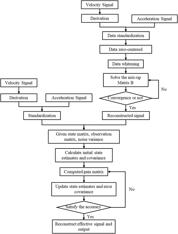
FIGURE 2. Flow chart of seismic velocity and acceleration signal combined denoising.

3 Results

3.1 Model data

A two-dimensional model was established (Figure 3A) to verify the joint denoising processing method for seismic velocity and acceleration signals. The wavelet of the velocity signal was the Riker wavelet with a dominate frequency of 20 Hz, and the wavelet of the acceleration signal was the derivative of the Riker wavelet with a dominate frequency of 20 Hz. Figure 3A shows the theoretical reflection coefficient, Figure 3B shows the synthesized velocity signal, Figure 3C shows the synthesized acceleration signal, and Figure 3D shows the acceleration signal obtained by this method. A comparison between shows that this method can obtain more accurate seismic signals without noise.

FIGURE 3

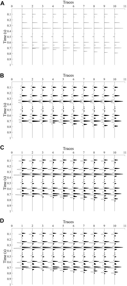
FIGURE 3. Comparison of the processing results of theoretical models (A). Theoretical reflection coefficient; (B). Synthesize velocity signal; (C). Synthetic acceleration signal; (D). Acceleration signal obtained.

The combined denoising method proposed in this paper was used to process the synthesized seismic record by adding Gaussian white noise with a SNR of 5 dB to verify the anti-noise ability of the method. Figures 4A, B show the velocity and acceleration signals, respectively, after adding noise, and Figure 4C shows the seismic acceleration signal obtained by this method. Figure 4D shows the residual difference between the original and processed acceleration signals. The comparison between Figure 3C, Figures 4C, D shows that the joint denoising method proposed in this paper can still separate accurate effective signals with the same Gaussian white noise.

FIGURE 4

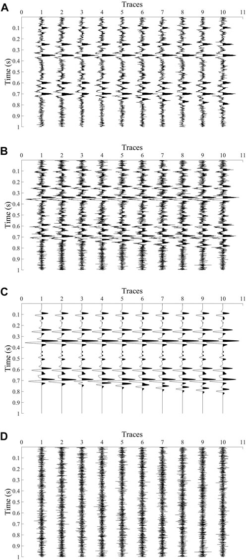
FIGURE 4. Comparison diagram of processing results of noisy data (A). Velocity signal with noise; (B). Acceleration signal containing noise; (C). Acceleration signal obtained; (D). Residual difference between original acceleration signal and processed acceleration signal.

Based on Figure 4, additional Gaussian white noise with a SNR of 15 is added to the synthesized acceleration signal, and the proposed joint denoising processing method was used to verify the anti-noise capability of this method. Figures 5A, B show the velocity signal after noise is added, and the acceleration signal after noise is added twice. Figure 5C shows the seismic acceleration signal obtained using this method. Figure 4D shows the residual difference between the original and processed acceleration signals. From Figure 3C, Figure 4C, Figure 5C, D, it can be seen that the joint denoising method proposed in this study can still separate accurate and effective signals containing mixed noise. Additionally, the SNR of the signals in Figures 5B, C were calculated to be 14.5 dB and 20.5 dB respectively, indicating that the proposed joint denoising method can significantly improve the SNR of the signal.

FIGURE 5

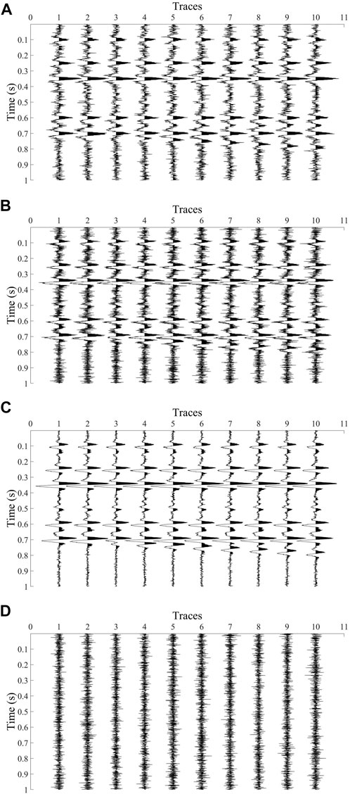
FIGURE 5. Comparison diagram of processing results of additional noisy data (A). Velocity signal with noise; (B). Acceleration signal with additional noise; (C). Acceleration signal obtained; (D). Residual difference between original acceleration signal and processed acceleration signal.

3.2 Field data

To further analyze the accuracy of this method and verify its effectiveness, we applied it to the velocity and acceleration signals of an offshore engineering area belonging to Sinopec Petroleum Engineering Geophysics Co. Figures 6A, B show the seismic velocity and acceleration shot gathers, respectively. Velocity and acceleration shot gathers are the signals received at the same position and time using velocity and acceleration geophones respectively. Figures 7A, B show the effective acceleration signal and filtered noise obtained by denoising using the method proposed in this paper respectively. After denoising, the continuity of the events in the seismic data is better. And there are fewer effective signals in the filtered noise.

FIGURE 6

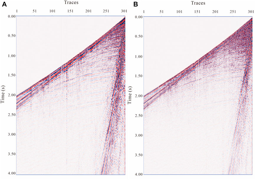
FIGURE 6. Shot gather (A). Velocity shot gather; (B). Acceleration shot gather.

FIGURE 7

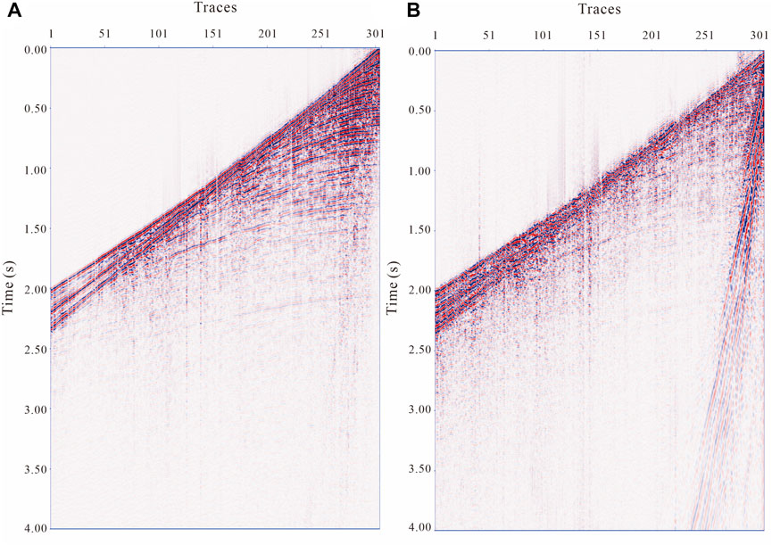
FIGURE 7. De-noising data (A). Processed acceleration shot gather; (B). Noise.

Figures 8A, B show the seismic velocity and acceleration profiles, respectively, while Figure 8C shows the seismic profile processed by the proposed method. Figure 9 shows the original acceleration profile and the noise filtered by the combined treatment. After processing, the continuity of the event in the seismic data is better, the event is compressed, and the structure is easy to recognize. Additionally, the weak seismic signal in the shallow layer of the seismic data was strengthened. The comparison results show the feasibility and practicability of this method for denoising seismic velocity and acceleration data. It can be seen from the filtered noise profile that although there are some effective signals in the noise filtered by this method, their amplitude is small, and their energy is weak, and most of the filtered noise results were incoherent. Figure 10 shows the frequency spectra of the original velocity profile, original acceleration profile, and processed profile. The yellow curve represents the original velocity profile spectrum, the red curve the original acceleration profile spectrum, and the black curve the profile spectrum after combined processing. From the spectrum of the data before and after processing, it can be seen that the proposed joint denoising method has almost no loss at low frequency. The dominate frequency of the signal was increased from 20 Hz to 40 Hz. The results show that the time resolution of the original velocity profile, the original acceleration profile and the processed profile are 10.9 m, 8.5 ms and 6 8ms, respectively. The time resolution was improved by approximately 20%, indicating that this method can significantly improve the time resolution of seismic data.

FIGURE 8

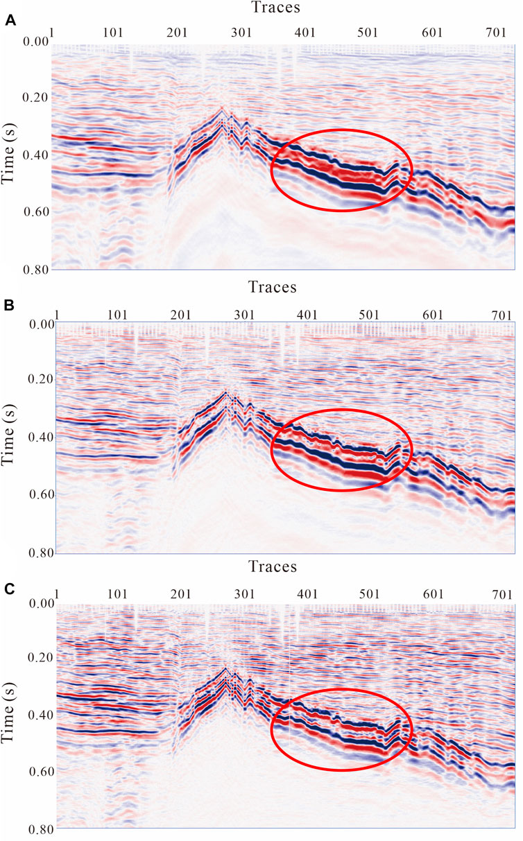
FIGURE 8. Joint processing results (A). Original velocity profile; (B). Original acceleration profile; (C). Processed acceleration profile.

FIGURE 9

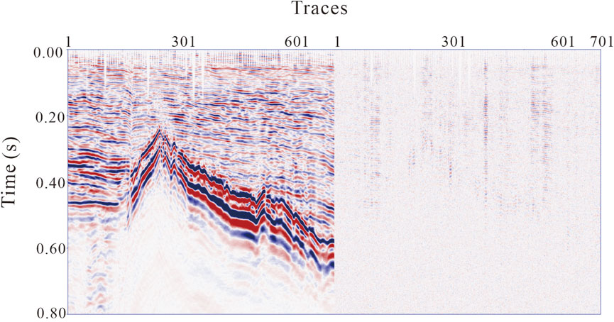
FIGURE 9. Comparison results before and after denoising (Left is the original acceleration signal; Right is noise removal).

FIGURE 10

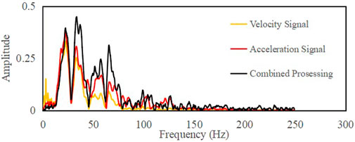
FIGURE 10. Spectrum of joint processing results (Yellow curve, original velocity profile spectrum; Red curve, original acceleration profile spectrum; Black curve, profile spectrum after combined processing).

To compare the advantages of joint processing, only a seismic acceleration signal was used for denoising. Figure 11 shows the seismic profile alone after noise removal; Figure 12 shows the original acceleration profile and filtered noise separately; and Figure 13 shows the spectrum of the seismic profile denoised using only acceleration signals. The time resolution of the seismic profile obtained using a single denoising processing method was 8 ms. This indicates that the effect of single denoising is weaker than that of combined denoising in terms of improving time resolution. Meanwhile, separate processing barely broadens the frequency band of the original data. Also, separate processing loses a part of the high-frequency information of the signal, while it can be observed that there are still many effective signals in the filtered noise profile. Finally, the joint denoising method is more sensitive to the identification of pinch-out points, and the event continuity is better.

FIGURE 11

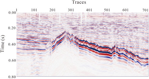
FIGURE 11. Separate processing result.

FIGURE 12

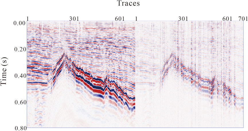
FIGURE 12. Comparison results before and after denoising (Left is the original acceleration signal; Right is noise removal).

FIGURE 13

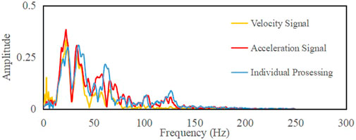
FIGURE 13. Spectrum of separate processing results (Yellow curve, spectrum of the original velocity profile; Red curve, original acceleration profile spectrum; Blue curve, profile spectrum alone after processing).

4 Discussion and conclusion

The joint denoising method presented in this paper relies on the system and observation equations, which are represented by the state transition matrix in the Kalman filter. The state transition matrix can typically be determined using either the average value method or the white noise method. In this study, the white noise method was chosen to determine the state transition matrix, owing to its simplicity and efficiency in calculation. Furthermore, when dealing with significant interference and low-dimensional data, the denoising results obtained using the average-value method may not accurately reflect the true situation, whereas the state-transition matrix determined using the white-noise method provides more reliable results. However, in joint denoising, the effect of Kalman filter is more dependent on the establishment of the observation system, that is, the effect of denoising is affected by the establishment of the state transition matrix.

The test results of model seismic data both with and without noise demonstrate that the method outlined in this paper is capable of effectively separating effective signals and enhancing the SNR. These results are consistent with the expected theoretical values. The processing of actual seismic data indicates that this method increases the signal bandwidth and time resolution. The proposed joint processing technique has numerous advantages over single-signal denoising, including a broadened bandwidth, improved time resolution, and greater continuity of events. Furthermore, this study highlights that combining different signal recording methods leads to a more accurate restoration of seismic wave signals, which will provide valuable insights for improving seismic acquisition techniques in the future.

Data availability statement

The data analyzed in this study is subject to the following licenses/restrictions: The dataset can be used with permission from the corresponding author. Requests to access these datasets should be directed to LY, youli@stu.cdut.edu.cn.

Author contributions

GZ, HbZ, LY, YY, and BZ developed and applied the method. GZ and HlZ supervised the funding for this study. All authors discussed the results and contributed to the final manuscript.

Conflict of interest

Author GZ was employed by the company Sinopec Petroleum Engineering Geophysics Co., Ltd. and Author HZ was employed by the company The Shengli Branch of the Sinopec Petroleum Engineering Geophysics Co., Ltd., and Author WC was employed by the company Sinopec Petroleum Engineering Geophysics Co., Ltd.

The remaining authors declare that the research was conducted in the absence of any commercial or financial relationships that could be construed as a potential conflict of interest.

This study was funded by the Research Project of Sinopec Petroleum Engineering Geophysics Co., Ltd. (“Research on seismic exploration technology based on acceleration signal,” SGC-2021-08; “Research on imaging technology of primary reflection and multiple waves of viscoelastic media based on ocean double geophone data,” SGC-2022-01). The funder was involved in the collection and processing of data.

Publisher’s note

All claims expressed in this article are solely those of the authors and do not necessarily represent those of their affiliated organizations, or those of the publisher, the editors and the reviewers. Any product that may be evaluated in this article, or claim that may be made by its manufacturer, is not guaranteed or endorsed by the publisher.

References

Bai, X. M., Yuan, S. H., Wang, Z. D., Chen, J. G., Wang, X. D., and Hu, Q. (2014). Digital geophones and exploration of tight Oil. A. 2014 SEG Annual Meeting.

Google Scholar

Cao, J. J., Wang, Y. F., and Yang, C. C. (2012). Seismic data restoration based on compressive sensing using regularization and zero-norm sparse optimization. J. Chin. J. Geophys. 55 (2), 239–251. doi:10.1002/cjg2.1718

CrossRef Full Text | Google Scholar

Cao, J. J., Zhao, J. T., and Hu, Z. Y. (2015). 3D seismic denoising based on a low-redundancy curvelet transform. J. J. Geophys. Eng. 12 (4), 566–576. doi:10.1088/1742-2132/12/4/566

CrossRef Full Text | Google Scholar

Chen, Y. K., Zu, S. H., Wang, Y. F., and Chen, X. H. (2019). Deblending of simultaneous source data using a structure-oriented space-varying median filter. J. Geophys. J. Int. 216 (2), 1805–1823. doi:10.1093/gji/ggaa189

CrossRef Full Text | Google Scholar

Damaševičius, R., Napoli, C., Sidekerskienė, T., and Woźniak, M. (2017). IMF mode demixing in EMD for jitter analysis. J. J. Comput. Sci. 22, 240–252. doi:10.1016/j.jocs.2017.04.008

CrossRef Full Text | Google Scholar

Denis, M. (2004). How digital sensors compare to geophones? A. CPS/SEG 2004 international geophysical conference. Berlin, Germany: Springer.

Google Scholar

Eikrem, K., Geir, J., and Morten, S. (2019). Iterated extended Kalman filter method for time-lapse seismic full-waveform inversion. J. Geophys. Prospect. 67 (2), 379–394. doi:10.1111/1365-2478.12730

CrossRef Full Text | Google Scholar

Hajsadeghi, S., Asghari, O., Mirmohammadi, M., and Meshkani, S. A. (2020). Discrimination of mineralized rock types in a copper-rich volcanogenic massive sulfide deposit through fast independent component and factor analysis. J. Nat. Resour. Res. 29 (1), 161–171. doi:10.1007/s11053-019-09499-0

CrossRef Full Text | Google Scholar

Han, J., and Van, D. B. M. (2013). Empirical mode decomposition for seismic time-frequency analysis. J. Geophys. 78 (2), 09–019. doi:10.1190/geo2012-0199.1

CrossRef Full Text | Google Scholar

Hons, M., Stewart, R., Lawton, D., Bertram, M., and Hauer, G. (2008). Field data comparisons of MEMS accelerometers and analog geophones. J. Lead. Edge 27 (7), 896–903. doi:10.1190/1.2954030

CrossRef Full Text | Google Scholar

Hons, M., Stewart, R., Lawton, D., and Malcolm, B. (2007). Ground motion through geophones and MEMS accelerometers: Sensor comparison in theory, modeling and field data. J. SEG Technical Program Expanded Abstracts.

CrossRef Full Text | Google Scholar

Joachim, W. (1997). A review of nonlinear diffusion filtering. J. Lect. Notes Comput. Sci. 1252 (1), 1–28. doi:10.1007/3-540-63167-4_37

CrossRef Full Text | Google Scholar

Lansley, M., Laurin, M., and Ronen, S. (2008). Modern land recording systems: How do they weigh up? J. Lead. Edge 27 (7), 888–894. doi:10.1190/1.2954029

CrossRef Full Text | Google Scholar

Liu, X. W., Gao, W., Zhang, N., and Liu, W. Y. (2007). ICA with banded mixing matrix based seismic blind deconvolution. J. Prog. Geophys. 22 (4), 1153–1163.

Google Scholar

Liu, Z. D., Lu, Q. T., Dong, S. X., and Chen, M. C. (2012). Research on velocity and acceleration geophones and their acquired information. J. Appl. Geophys. Springer. 9 (2), 149–158. doi:10.1007/s11770-012-0324-6

CrossRef Full Text | Google Scholar

Meng, H. J., Su, Q., Zeng, H. H., Xu, X. R., Liu, H., and Zhang, X. M. (2021). Blind source separation of seismic signals based on ICA algorithm and its application. J. Lithol. Reserv. 33 (4), 93–100.

Google Scholar

Mirko, B., and Maiza, B. (2009). Random and coherent noise attenuation by empirical mode decomposition. J. Geophys. 74 (5), 89–98. doi:10.1190/1.3157244

CrossRef Full Text | Google Scholar

Morlet, J., Arens, G., Fourgeau, E., and Giard, D. (1982). Wave propagation and sampling theory—Part II: Sampling theory and complex waves. J. Geophys. 47, 222–236. doi:10.1190/1.1441329

CrossRef Full Text | Google Scholar

Necati, G. (1986). F-X decon and complex wiener prediction filter. A. 1986 SEG Annual Meeting.

Google Scholar

Nicolas, T., and Jérôme, L. (2017). Understanding MEMS based digital seismic sensors. J. First Break. 35 (1), 93–100.

Google Scholar

Ott, N., and Meder, H. G. (1972). The Klaman filter as a prediction error filter. J. Geophys. Prospect. 20 (3), 549–560. doi:10.1111/j.1365-2478.1972.tb00654.x

CrossRef Full Text | Google Scholar

Perona, P., and Malik, J. (1990). Scale-space and edge detection using anisotropic diffusion. J. IEEE Trans. Pattern Analysis Mach. Intell. 12 (7), 629–639. doi:10.1109/34.56205

CrossRef Full Text | Google Scholar

Qin, F. L., Liu, J., and Yan, W. Y. (2018). The improved ICA algorithm and its application in the seismic data denoising. J. J. Chongqing Univ. 17 (4), 162–170.

Google Scholar

Ren, L. G. (2018). Analysis and application of velocity and acceleration geophone's seismic response characteristic. J. Prog. Geophys. 33 (5), 2159–2165.

Google Scholar

Saruwatari, H., Kawamura, T., Nishikawa, T., Lee, A., and Shikano, K. (2006). Blind source separation based on a fast-convergence algorithm combining ICA and beamforming. J. Speech Lang. Process. 14 (2), 666–678. doi:10.1109/TSA.2005.855832

CrossRef Full Text | Google Scholar

Sergio, L. M. F., and Tad, J. U. (1988). Application of singular value decomposition to vertical seismic profiling. J. Geophys. 53 (6), 778–785. doi:10.1190/1.1442513

CrossRef Full Text | Google Scholar

Spanias, A. S., Jonsson, S. B., and Stearns, S. D. (1991). Transform methods for seismic data compression. J. IEEE Trans. Geoscience Remote Sens. 29 (3), 407–416. doi:10.1109/36.79431

CrossRef Full Text | Google Scholar

Wang, J., Zhang, J. H., Yang, Y., and Du, Y. S. (2021). Anisotropic diffusion filtering based on fault confidence measure and stratigraphic coherence coefficients. J. Geophys. Prospect. 69 (5), 1003–1016. doi:10.1111/1365-2478.13085

CrossRef Full Text | Google Scholar

Wang, W., Gao, J. H., and Chen, W. C. (2012). Random seismic noise suppression via structure-adaptive median filter. J. Chin. J. Geophys. 55 (5), 1732–1741. doi:10.6038/j.issn.0001-5733.2012.05.030

CrossRef Full Text | Google Scholar

Wei, J. D. (2018). Comparison of recording accuracy between analog geophone and MEMS accelerometer and their influence to the S/N ratio. Prog. Geophys. 33 (4), 1726–1733. doi:10.6038/pg2018CC0018

CrossRef Full Text | Google Scholar

Zhang, H. B., Li, L. M., Zhang, G. D., Zhang, B. H., and Sun, M. M. (2020). Seismic acceleration signal analysis and application. J. Appl. Geophys. 17 (1), 67–80. doi:10.1007/s11770-020-0802-1

CrossRef Full Text | Google Scholar

Zhang, H. L., Zhang, G., Xue, B., and Yuan, J. W. (2022). Mainlobe jamming suppression via improved BSS method for rotated array radar. J. J. Syst. Eng. Electron. 33 (6), 1151–1158.

Google Scholar