 Peiyu Miao
 Genru Xiao1,2*
 Keliang Zhang
94% of researchers rate our articles as excellent or good
Learn more about the work of our research integrity team to safeguard the quality of each article we publish.
Find out more
ORIGINAL RESEARCH article
Front. Earth Sci., 16 May 2023
Sec. Solid Earth Geophysics
Volume 11 - 2023 | https://doi.org/10.3389/feart.2023.1176241
This study investigated the effects of various seasonal fitting techniques on the spatial distribution of the common mode errors taking the coordinate time series of the continuous GPS reference stations of the Crustal Movement Observation Network of China (CMONOC) as an example. First, the seasonal term of coordinate time series was calculated using constant amplitude harmonic fitting (CAF), continuous wavelet transform (CWT), and smoothing spline fitting (SPF). The seasonal term and linear trend were then removed to obtain the residual time series. Finally, to determine the common mode errors of residual time series, principal component analysis (PCA) was applied. The results indicate that 1) smoothing spline fitting is superior to constant amplitude harmonic fitting and continuous wavelet transform in its ability to fit short-term irregular seasonal signals. In comparison to constant amplitude harmonic fitting, N/E/U has root mean square error (RMSE) values of smoothing spline fitting that are lower by 25%, 20%, and 14.4%, respectively. Smoothing spline fitting also has a higher coefficient of determination than continuous wavelet transform and constant amplitude harmonic fitting. The coefficient of determination in the U direction is larger than that in the N and E directions. 2) Each order PC of the residual series fitted by smoothing spline fitting exhibits apparent spatial aggregation characteristics, with PC1 having a uniform spatial distribution and presenting a largely positive response. Nevertheless, the residual series obtained by constant amplitude harmonic fitting and continuous wavelet transform exhibits scattered spatial response distribution features in each order PC. Compared to N and E, U’s spatial response distribution is distinct. From north to south, the spatial response of PC1 in the U direction progressively diminishes. In addition to being much lower than that in other locations, the Sichuan–Yunnan region’s spatial response value of PC1 and PC3 also exhibits a clear negative reaction. The root mean square error value of the residual series after smoothing spline fitting is the least, and the filtering effect is the best when comparing the spatial filtering effect based on the three fitting methods. We also compared the root mean square error reduction ratio before and after spatial filtering, and the results showed that the root mean square error reduction ratio before and after the residual series obtained by smoothing spline fitting is slightly larger than that obtained by other methods.
There are some spatial correlation errors in the coordinate time series of the GPS network; this type of geographically related noise is known as common mode errors (CME). The CME presented in the GPS coordinate time series is vital for the study of errors similar to those caused by GPS technology as well as for assessing the effects of environmental loading and GPS velocity uncertainty (Blewitt and Lavallée, 2002; Bogusz and Klos, 2016; Abraha et al., 2017). By effectively reducing the GPS common mode errors, the coordinate time series signal-to-noise ratio may be improved and crustal deformation features can be accurately predicted (He et al., 2017). GPS coordinate residual common mode components do not always represent errors; they might also contain regional structural signals. CME can be caused by regional differences in water and atmosphere, faults in the reference frame, errors in the GPS satellite orbit, etc., (Wang et al., 2017) all of which are typically removed by filtering methods in data processing. Numerous researchers have recently suggested various CME filtering methods, including the regional stacking filtering method, which was first proposed by Wdowinski et al. (2017) and can significantly increase the signal-to-noise ratio (SNR) of the series; it has limitations when it comes to extracting CME because it requires that each station have an equal CME, yet studies have shown that the spatial distribution of CME is variable. Later, other researchers enhanced the regional stacking filtering method by using the inter-station distance and the series length as the pertinent weights (Márquez-Azúa and DeMets, 2003). The stacking filtering technique is more suited for small-area spatial filtering. The commonly used technique for spatial filtering, principal component analysis (PCA) with Karhunen–Leove (KLE), was presented by Dong et al. (2006). However, it requires that the GPS network has the same time scale. He et al. (2015) calculated the coordinate displacements of atmospheric pressure, soil moisture, snow depth, and non-tidal ocean-induced environmental loading for the Cascadia and Southern California regions, respectively, and then eliminated the regional CME of the residual series based on the PCA method, demonstrating that the PCA-based territorial spatial filtering can successfully eliminate the CME and reduce uncertainty. Li et al. (2019) used PCA to extract CME from 41 GPS stations in Southern California, proving that spatial filtering can effectively lower GPS time series root mean square error and that getting rid of CME can raise velocity field estimation believability. Tan et al. (2020) used QOCA to remove offset, linear trend, annual, and semi-annual term signals from coordinate time series over a period of almost 6 years in the Sichuan–Yunnan region of China. They then performed PCA decomposition on the residual series to obtain the regional CME and evaluated the CME using power spectrum analysis. Xu et al. (2022) demonstrated that CME is a non-negligible component of velocity field extraction in the area by using PCA and KLE methods to assess the CME of GPS residual series in the Mount Everest region while eliminating the linearly variable, annual, and semi-annual term signals. In addition to the PCA method, independent component analysis (ICA) is another option that can incorporate CME’s higher-order statistical data for spatial filtering. Ming et al. (2017) removed the linear trend and seasonal variation from the long-span time series of CMONOC by spatially filtering the residual series using the methods of stacking, PCA, and ICA, respectively. The results demonstrated the effectiveness of the ICA method in identifying anomalous stations and suggested an ICA-based definition of CME.
Seasonal signals and random noise present in the series have an impact on velocity estimations obtained from coordinate time series of continuous GPS stations. The time series cannot be effectively characterized if the deterministic model of a linear trend and periodic term is not sufficiently precise (Klos et al., 2018). The series noise model will be judged in an unsatisfactory manner if the seasonal signal is estimated incorrectly. Gu et al. (2017) compared the vertical coordinate time series of 224 GPS stations in mainland China with the ground load model and showed that the vertical seasonal deformation could be partly explained by the redistribution effect of environmental quality, but some unmodeled signals were still retained in the residual series. Li et al. (2020a) focused on seasonal mass changes in North China using GRACE data, surface load model data, and coordinate time series of 30 GPS stations in CMONOC. They found that although the annual and semi-annual signals evaluated by least squares have a good correlation with the vertical displacements of GRACE and surface loading models (SLM), they are unable to accurately reflect the seasonal mass changes. These studies demonstrate that the annual cycle and semi-annual cycle of least squares estimation can approximately characterize the seasonal variation of the time series to some extent, but the seasonal fluctuation of the time series is not a simple harmonic form, which will introduce new errors to the residual series and affect the extraction of CME.
When obtaining seasonal term signals and CME, most researchers often use the following three techniques: the first is to model the seasonal term signal in the coordinate time series using a harmonic model with constant amplitude, phase, and simple parameters and then separate the CME for the residual series after removing the trend and seasonal terms. However, this method may result in inaccurate modeling of seasonal signals because some seasonal signals enter the residual series, which affects the CME extraction. The second is to eliminate the seasonal signal component so that environmental loading can be used to interpret it using GRACE data, environmental loading models, etc. This approach will momentarily cause certain signals that the geophysical model cannot account for, as well as error signals produced by the inaccurate environmental loading model, to enter the residual series, leading to an error in the CME extraction. The third is removing the linear trend term from all the series, finding the correct geophysical interpretation for the extracted main components, then examining the relationship between the main components and different loading models, and identifying the primary geophysical factors influencing the seasonal fluctuations of coordinate time series in a particular area. Wang et al. (2020) demonstrated that the PCA approach could extract regional common mode errors in China and increase the SNR of time series by performing common mode error analysis on residual series after tectonic movement signals and seasonal signals were subtracted. To predict the seasonal signals of GPS coordinate time series, Liu et al. (2020) presented a method based on ICA and variable coefficient regression, and they then applied it to the vertical time series of 262 IGS stations around the world. The findings demonstrated that this approach could successfully replicate the seasonal fluctuations in vertical time series and was noticeably superior to least squares fitting. Different fitting methods can reflect seasonal signal fluctuations more accurately and obtain more accurate residual series.
The Crustal Movement Observation Network of China (CMONOC) is an observation network based on satellite navigation and positioning system (GNSS) observation, which is primarily used to track changes in the gravity field morphology, crustal movement, and other phenomena on the Chinese mainland. It has 260 continuous GNSS reference stations that can provide observation data sampled every 30 s. Consequently, in this paper, based on CMONOC data over 10 years in time, we employed constant amplitude harmonic fitting (CAF), continuous wavelet transform (CWT), and smoothing spline fitting (SPF) to estimate seasonal components in time series after acquiring the coordinate time series by PPP processing. After excluding seasonal variations, CME is thought to be the most common error. The effects of different fitting methods on the geographic distribution of CME were examined and compared to the spatial filtering effects.
We processed the GPS observation data carefully to get the coordinate time series of each station based on ITRF2014 in this study using the GIPSY-OASIS software package, which was created by NASA’s Jet Propulsion Laboratory (JPL). We used continuous observation data from 260 CMONOC continuous GPS stations (Figures 1, 2). Due to the influence of the atmosphere and other variables, the coordinate time series may contain some blatantly incorrect data that plainly deviate from a linear trend or periodic change. Using the
where
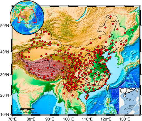
FIGURE 1. Distribution of 260 stations.
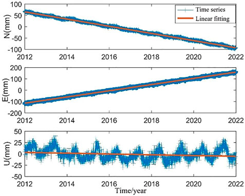
FIGURE 2. Coordinate time series of YNYL station and its linear fitting. Blue indicates that the coordinate time series removed the error data, and red line indicates least square linear fitting.
The GPS continuous stations coordinate time series comprises structural data, seasonal term data, co-seismic displacement brought on by earthquakes, and post-earthquake displacement signals, among others (Zhao et al., 2015). The trend term and step signal have been removed by the aforementioned data preparation process. In this work, CWT, SPF, and CAF each will be used to match the seasonal term signal.
According to earlier research, the annual and semi-annual term signals in the GPS coordinate time series were frequently represented as harmonic functions with constant amplitude and phase as follows:
Here,
Wavelet analysis, an analysis method with both time and frequency characteristics, can be applied to fit seasonal terms of GPS coordinate time series (Pugliano et al., 2016). The wavelet transform, which approximates the continuous signal with finite resolution as a step function and conveys the signal through a wavelet function system, is the foundation of wavelet analysis. The fundamental wavelets are scaled and displaced to produce all wavelets. Let
We refer to this fundamental wavelet
where
To deconstruct the time series data in this paper with the trend term and step term eliminated, we chose coif 5, one-dimensional wavelet. A total of eight layers are then decomposed to produce detailed signals. The symmetry of the wavelet coif 5 is superior. The fitting value for the residual series is the sum of the seventh layer (d7) and the eighth layer (d8). Figure 3 illustrates the wavelet decomposition of the YNLJ station using this method as an example.
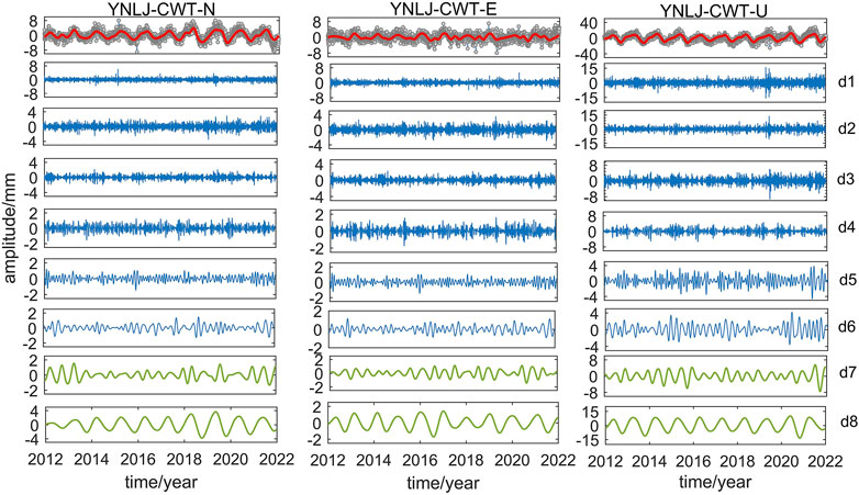
FIGURE 3. Continuous wavelet decomposition diagram of YNLJ station. The gray point represents the detrended time series, the red line represents the fitting value of CWT, and the green line represents the signals of the seventh and eighth layers of the wavelet decomposition.
Seasonal signals are also fitted using the smoothing spline fitting approach in addition to the continuous wavelet transform. Smoothing spline can be used to fit discrete functions. The value of the following formula can be minimized by selecting the most appropriate function among all the functions with second continuous derivatives. RSS can be understood as the penalty coefficient:
where
In the fitting process,
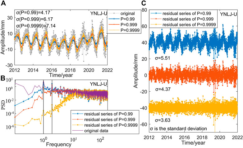
FIGURE 4. SPF of YNLJ in the U direction. (A) Fitting value in the U direction of the YNLJ station when the smoothing coefficients are 0.99, 0.999, and 0.9999, respectively; (B) power spectrum of the residual series of the YNLJ station in the U direction after removing the seasonal term by SPF; (C) residual series of the YNLJ station after fitting seasonal terms with the smoothing coefficients of 0.99, 0.999, and 0.9999, respectively, where σ is the standard deviation.
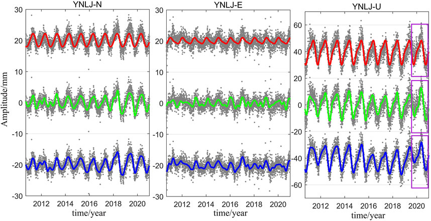
FIGURE 5. Seasonal time series fitting of YNLJ. Red line indicates CAF, shifted upward by 20 mm; green line indicates CWT; blue line indicates SPF, shifted down by 20 mm in N/E. The distance parallel to the U direction is 40 mm.
To evaluate the fitting effects, the commonly used indicators are the coefficient of determination
The coefficient of determination
Here,
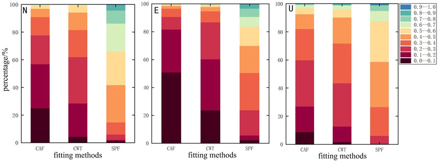
FIGURE 6. Cumulative probability graph of the coefficient of determination
The coefficient of determination
The N/E/U direction time series of more than 260 stations in CMONOC are fitted by the aforementioned three methods, and the fitting effect is measured by the RMSE value, which is expressed as:
Here,
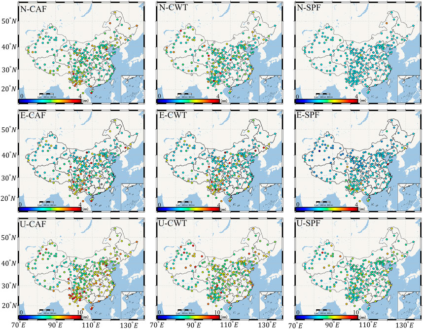
FIGURE 7. RMSE value of each station in the N/E/U direction. The first row from left to right is the RMSE of CAF, CWT, and SPF in N, respectively; the second row from left to right is the RMSE of CAF, CWT, and SPF in E, respectively; the first row from left to right is the RMSE of CAF, CWT, and SPF in U, respectively. The color indicates RMSE values.
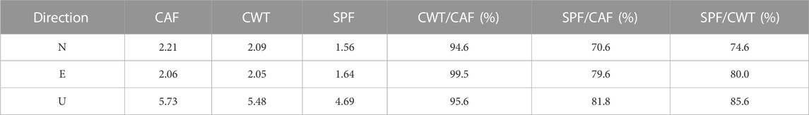
TABLE 1. Mean RMSE of the three fitting methods for each station in the N/E/U direction.
The RMSE value of each station in Figure 7 ranges from 0 to 4 mm in the N/E directions and from 0 to 10 mm in U. The average RMSE values of the N/E/U directions were, respectively, 2.21, 2.09, and 1.56 mm; 2.06, 2.05, and 1.64 mm; and 5.73, 5.48, and 4.69 mm. In the N/E directions, the fitting effect of CAF and CWT is close, and the RMSE value of CWT is slightly smaller than that of CAF in the Sichuan–Yunnan area. The RMSE value of SPF is the smallest, which indicates that SPF in the N/E direction can better fit the seasonal fluctuations of the station coordinates. In the U direction, the proportion of stations with RMSE in the range of 5∼7 mm and 7∼10 mm in CAF was 54.6% and 17.5%, respectively. The proportion of stations with RMSE in the range of 5∼7 mm and 7∼10 mm in CWT was 48.2% and 13.2%, respectively. The RMSE values of SPF in the aforementioned range of sites are 26.7% and 1.2%, respectively, indicating that SPF is significantly better than CWT and CAF.
Generally, time series consist of the long-term trend term, the seasonal term, and the irregular residual term:
where
In the aforementioned formula,
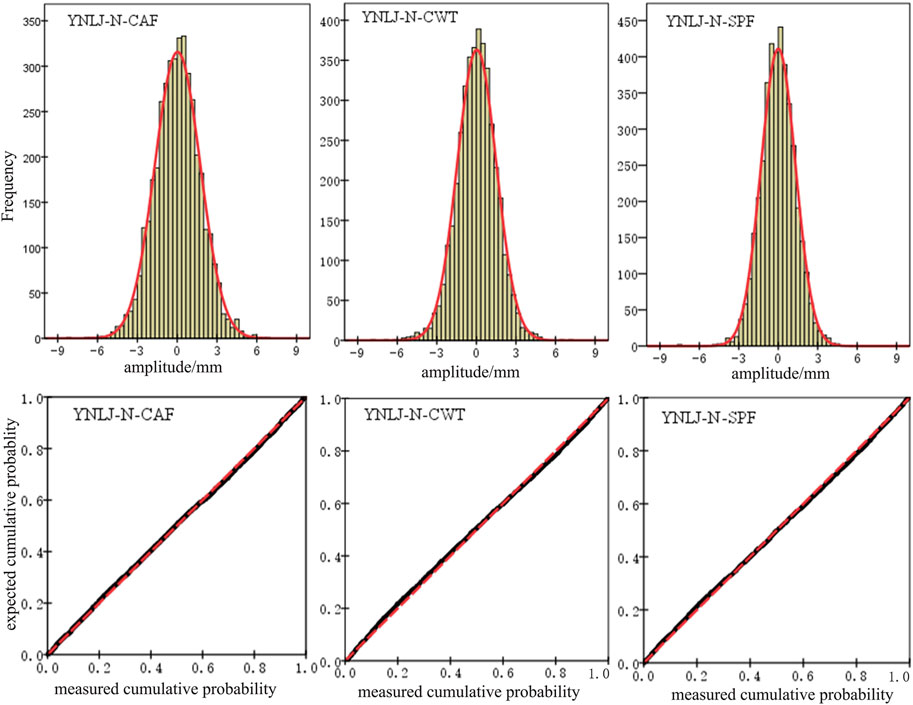
FIGURE 8. Histograms and normal P–P plots for YNLJ in N direction. The first row shows histograms, with the red line indicating the normal distribution; the second row shows the normal P–P plots, with the red dashed line indicating the normal trend line.
The Pearson correlation coefficient was used to calculate the inter-station correlations. Taking 20 stations in the first phase of the CMONOC as an example, the inter-station correlation is shown in Figure 9. The inter-station correlation coefficient of the residual series of the other stations is positive, whereas it is negative for the residual series of CHUN-DLHA, BJFS-KMIN, DLHA-HRBN, DLHA-JIXN, and KMIN-LHAS. The correlation coefficients of the residual series between stations are relatively close when the seasonal factor is fitted with CAF and CWT. The residual series tend to be more stable when using SPF because it is better able to account for the amplitude modulation phenomenon in the seasonal term of coordinate time series. This increases the inter-station correlation coefficient of some station residual series, and the calculated inter-station correlation coefficient is greater than 0.3, indicating that there is some pertinence between the reference stations.
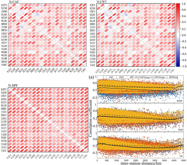
FIGURE 9. Correlation coefficients between different stations in the N direction. The first row shows the inter-station correlation based on CAF and CWT from left to right, and the second row shows the inter-station correlation based on SPF. (A) Correlation coefficients between the residual time series of different stations. The inter-station correlation coefficients of CAF/CWT/SPF are shown as blue/red/yellow dot marks, respectively. Moreover, they are smoothed and shown as the black straight line, black dot crossed line, and black dotted line, respectively.
The inter-station correlation of the residual coordinate time series is usually related to the environment of the reference station, the data processing method, and other factors (Yuan et al., 2018). As shown in Figure 9A, we determined the residual series inter-station distance and inter-station correlation coefficient in the N/E/U direction for each station. The correlation coefficient between the residual series of stations showed a downward trend as the distance between stations increased overall, but not all stations followed this rule; the correlation coefficient between a few stations is less than zero in places where the distance between stations is less than 500 km, demonstrating that factors other than distance play a role in determining the correlation between stations. By comparing the effects of the residual series obtained by the three different seasonal term fitting methods on the calculation of inter-station correlation, the correlation of the residual series obtained after SPF fitting the seasonal term is more aggregative, and the inter-station correlation of the residual series obtained by SPF in the N/E/U directions is greater than the inter-station correlation of the two other methods.
Following various seasonal term fitting methods in N/E/U, Table 2 displays the inter-station correlations of the residual series. In the N/E direction, more than 50% of inter-station correlations are more than 0.3, and most inter-station correlations in the U direction fall between 0 and 0.3. The percentage of negative inter-station correlations in the three directions can be greatly decreased using the residual series acquired using the seasonal term fitting approach with SPF. The inter-station correlation of the residual series is significantly increased by SPF methods in the N/E direction, and the inter-station correlation coefficient is decreased when SPF increases the proportion of inter-station correlation between 0 and 0.3 in the U direction.
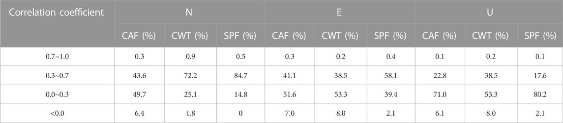
TABLE 2. Correlation coefficient between the residual time series based on different fitting methods in the N/E/U directions.
Principal component analysis (PCA) is typically used to adjust for CME in residual coordinate series. The calculation of CME is based on inter-station correlation; the greater the correlation, the higher the value of CME. The elimination of CME can weaken the inter-station correlation of the GPS network. We select the PCA approach as the spatial filtering method to extract CME because it can directly extract CME from each station without the need for a priori assumptions (Shen et al., 2014; Zheng et al., 2021). The PCA method is a decomposition method that constructs an orthogonal basis based on the data itself. Reducing dimensionality while retaining as many of the dataset variation characteristics as possible is the main goal of the spatial filtering of the PCA method. A coordinate time series can be divided into several mutually orthogonal modes using the PCA approach, which is based on second-order statistics. If the time series for each station are aligned, the following matrix can be obtained:
Decompose the aforementioned matrix as follows:
where
The column vector in
where
By arranging
where
The PCA method decomposes the time series into temporal principal components and spatial eigenvectors. The variation characteristics of the first few principal components can reflect the common variation of the residual series over time at each station, and the eigenvectors can reflect the spatial distribution characteristics of the strength of the variation over time. The CME of GPS continuous time series in mainland China was obtained by the PCA method. We analyze the effects of various seasonal term fitting methods on the extraction of the CME and analyze the spatial response distribution characteristics of the CME of the CMONOC. The concept of CME has been widely used in GPS networks, but there is no clear definition of CME, and we regard the spatial noise after removing the constructive and seasonal signals as CME. From among the more than 260 stations in the CMONOC, we chose stations with data integrity rates of more than 85% (223) and used the cubic spline interpolation approach to complete the missing residual series data. PCA was used to process the residual series of 4,064 epochs between 2010.8015 and 2021.9829 to determine CME.
Figure 10 represents the cumulative contribution rate of the first 30 orders of PC extracted from the PCA of the residual series in the N/E/U direction, where the cumulative contribution rate of the PCA of the residual series is obtained by fitting the seasonal term to the CAF. The contribution rate of PC1, PC2, and PC3 was 41.39%, 6.23%, and 4.30% in the N; 28.94%, 8.76%, and 5.76% in the E; and 22.55%, 7.72%, and 6.16% in the U. The contribution rate of PCA of residual series obtained by fitting seasonal signal with CWT was 40.54%, 6.76%, and 4.50% in the N; 27.68%, 9.64%, and 5.42% in the E; 22.52%, 7.47%, and 5.73% in the U. The contribution rate of PCA of residual series obtained by fitting seasonal term with SPF was 43.61%, 3.11%, and 2.47% in the N; 36.11%, 6.59%, and 4.34% in the E; and 21.18%, 6.79%, and 4.87% in the U. Comparatively, N is the largest, followed by E, and U is the smallest among them in the relationship of the contribution rate of each order of PC in three directions. The variance contribution rate of the first three orders of PC is greatly increased by the seasonal term fitting approach with SPF in the E direction. Due to the small cumulative contribution rate, the first fifth-order PC is chosen to calculate the common mode errors in the U direction.
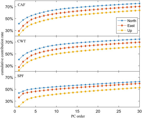
FIGURE 10. Top 30 major component cumulative contribution rate in the N/E/U direction. The figures in the top, middle, and bottom rows, respectively, represent the cumulative contribution rates of each order of PC to the residual series after fitting seasonal signals based on CAF, CWT, and SPF. Blue, red, and yellow denote the N, E, and U directions, respectively.
CME is a kind of error with spatial characteristics. If the principal components are only calculated based on the variance contribution rate, some PCs with low eigenvalues but clear spatial responses will be overlooked (Xu et al., 2022). Therefore, we examined the corresponding spatial responses of each order of primary components. The SR and PC series for the first three orders of PCs at each station, using the N direction as an example, are displayed in Figure 11. The PC series represent changes in time, and the SR indicates the degree of response of that station. A positive SR shows a positive response of a station to a particular PC, whereas a negative SR value indicates that the station responds negatively to a particular PC. The first three orders of PC retrieved by CAF and CWT are comparable in terms of the time domain: PC1 fluctuates less than PC2 and PC3, and PC2 and PC3 exhibit nonlinear variation characteristics. The first three order PCS that SPF was able to extract are all depicted as quite stable series. A rather uniform positive spatial response was seen in PC1 produced by CAF, CWT, and SPF, with mean response values of 71%, 71%, and 76%, respectively, and no discernible variation in the magnitude of response values. The spatial responses of PC2 and PC3 of CAF and CWT exhibit relative heterogeneity without obvious spatial clustering phenomena. The SR values of PC2 and PC3 of SPF show spatially complementary distributions, with the SR values of PC2 showing a positive response in the western block and a larger negative response in the coastal region, and the SR values of PC3 showing a positive response in the Sichuan–Yunnan region and southern Qinghai–Tibet and a significant negative response in the northeastern block. These two-order PCs show small spatial responses at the junction of positive and negative SR values. Using the N direction as an example, the analysis shows that the residual series obtained by SPF are able to obtain the spatial distribution characteristics of the common mode errors by PCA. The investigation reveals that the residual series acquired by SPF are capable of obtaining the spatial distribution properties of CME by PCA.
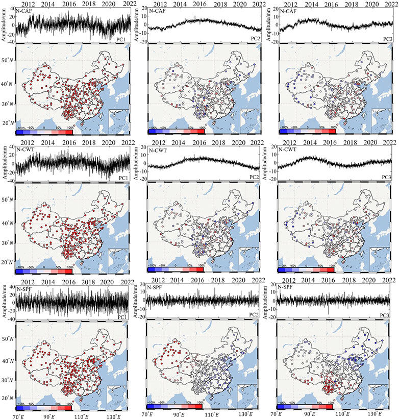
FIGURE 11. First three PCs and their corresponding SR after fitting the seasonal terms with three methods in the N direction. From the top to the bottom: in the first row, PC1, PC2, PC3 and their SR based on constant amplitude harmonic fitting (CAF), respectively, are given; in the second row, PC1, PC2, PC3 and their SR based on continuous wavelet transform (CWT) fitting, respectively, are given; in the third row, PC1, PC2, PC3 and their SR based on smoothing spline fitting (SPF), respectively, are given.
Figure 12 represents a histogram of the normalized spatial response values for the first fifth-order PC of the residual series after fitting the seasonal term by the three fitting methods in the N direction, where it can be seen that all stations have positive SR values for PC1, mostly within the range of 50%–100%. According to the statistical histograms and spatial distribution maps of SR2 and SR3 for each station, the CAF and CWT exhibit high symmetry, whereas SPF shows poor symmetry, which suggests that the statistical histogram is smaller and less symmetrical when SR has a distinct spatial distribution. In Figure 12, we can see that SR2 and SR3 extracted by SPF combined with the PCA method have spatial classification characteristics, and they have histograms with SR values for PC4 primarily around 0, indicating that PC4 should not be included in the CME of the stations. By analyzing the N direction, we can see that the method of SPF to obtain the residual series has better spatial clustering characteristics by calculating the SR value of each order of PC through PCA. Since the CME itself is a spatially comparable noise, the SPF approach is selected to prevent the seasonal signal from influencing the residual series. To create the residual series for the E and U directions, we also fit the seasonal term using SPF. PCA was then used to create the principal component series and the spatial response values for each station.

FIGURE 12. SR statistical histogram of first fifth-order PC in the N direction. From the top to the bottom: in the first row, SR1, SR2, SR3, SR4, and SR5 based on CAF, respectively, are given; in the second row, SR1, SR2, SR3, SR4, and SR5 based on CWT, respectively, are given; in the third row, SR1, SR2, SR3, SR4, and SR5 based on SPF, respectively, are given.
Figure 13 shows the first three orders of PC and SR values extracted by PCA in E direction. Principal component series showed strong temporal stability, with the PC1 series value being significantly higher than PC2 and PC3. Space-wise, SR values in the E and N directions exhibit comparable patterns of spatial distribution: SR1 is positive, indicating that PC1 is a common component of CME. The spatial distribution of SR2 reveals a gradient change from coastal to inland, with the SR values showing a negative spatial response and a greater degree of response the closer the coastal area. The SR value shifts from negative to positive as the longitude shrinks, and the degree of spatial responsiveness gradually reduces before trending bigger. In SR3, the Sichuan–Yunnan region exhibits a positive spatial response, while the northeast and western regions exhibit a negative spatial response.
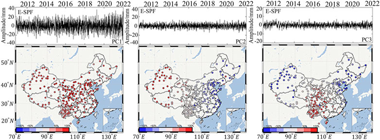
FIGURE 13. First three order of PCs and their SRs in the E direction. From the left to the right, PC1, PC2, PC3 and their SRs in E based on SPF, respectively, are given. The diagrams in the top row show the PC series diagram, and the diagrams in the bottom row show the spatial distribution of SR.
Figure 14 shows the first fifth-order PC and SR values extracted by PCA in the U direction. In the time domain, the magnitudes of the first 5 orders of PC series values are in the following order: PC1 is the largest, followed by PC2/PC3, and PC4/PC5 is the smallest. Spatially, the distribution of SR values in the U direction shows different spatial distribution characteristics from those in the N and E direction. SR1 exhibits an overall positive response, and unlike the N/E direction, the response values in the U direction gradually decrease from north to south, with a noticeably smaller response to PC1 in the Sichuan–Yunnan area. In SR2, only the western block shows a significant positive spatial response. In SR3, the northeastern block exhibits a large positive spatial response, while the Sichuan–Yunnan block exhibits a large negative spatial response. In SR4, the northern and coastal regions of the western block exhibit a largely negative response, and areas such as Gansu and Ningxia show a largely positive response. In SR5, the northeastern region exhibits a relatively large negative spatial response. With no particularly large and homogeneous SR values in the first five orders of PC, the spatial response of each order of PC in the U direction for the Sichuan–Yunnan area is completely different from the distribution features in the N/E direction. Since CME is an error with spatial characteristics, the distribution of spatial responses should be considered together with the variance contribution.
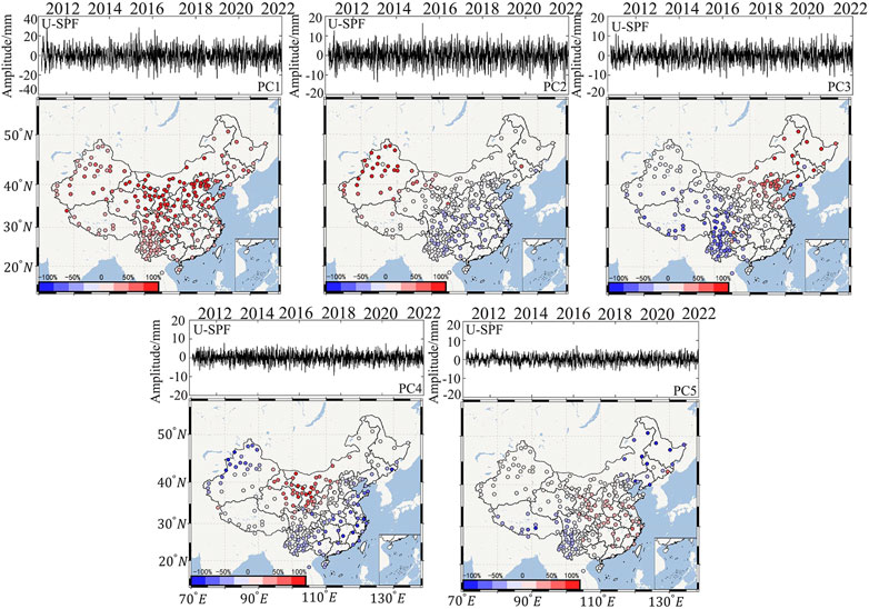
FIGURE 14. First five PCs and their SRs in the U direction. From the left to the right, from the top to the bottom, PC1, PC2, PC3, PC4, PC5 and their SR in U direction based on SPF, respectively, are given. The diagrams in the top row show the PC series diagram, and the diagrams in the bottom row show the spatial distribution of SR.
In this paper, CAF, CWT, and SPF are used to fit the seasonal term signals in the coordinate time series, and the three kinds of residual series are spatially filtered using the PCA method. The RMSE value is used to measure the discretization of residual series, and the RMSE reduction value is used to measure the spatial filtering effect of PCA method. The RMSE reduction can be calculated using the following equation (Li et al., 2020b):
The RMSE reductions are depicted in Figure 15. With an average RMSE reduction of 24.3%, 8.19%, and 7.34% in the N/E/U direction of the residual series after CAF, 17.6%, 22.5%, and 7.45% in the N/E/U direction of the residual series after CWT, and 26.8%, 24.2%, and 7.78% in the N/E/U direction of the residual series after SPF, the spatial filtering somewhat reduced the RMSE in all the directions. Among the three fitting methods, SPF has the best fitting effect and the smallest RMSE value, and the reduction ratio of RMSE value after PCA spatial filtering is higher than that of the other two fitting methods. The RMSE value of residual series after filtering is the smallest. Compared with the spatial filtering effect of the PCA method on the three directions, the RMSE reductions in the N/E direction are mostly in the range of 10%–40%, and the RMSE reductions in the U direction are mostly in the range of 0%–15%, indicating that the spatial filtering effect of the PCA method on residual series in the U direction is slightly worse than that in the N/E direction.
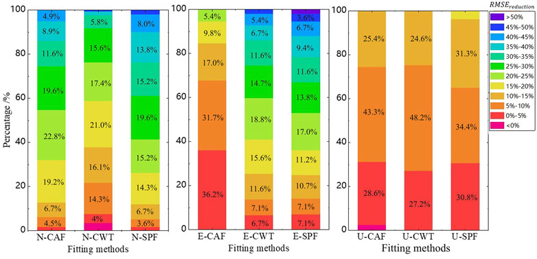
FIGURE 15. Cumulative probability graph of RMSE reduction for residual series using three methods in each direction. The graph represents the ratio of the number of stations to the total number of stations within the range of
In this paper, high-precision data processing is carried out to obtain coordinate time series from CMONOC, and the seasonal terms are fitted using constant amplitude harmonic fitting, continuous wavelet transform, and smoothing spline fitting, respectively, after which CME is extracted from the residual series by PCA, and the effects of different seasonal term fitting methods on the spatial distribution of the CME are analyzed. The following conclusions are obtained:
(1) To take into account the seasonal amplitude modulation, the fitting effects of the three fitting methods were compared. By comparing the coefficient of determination
(2) Following the removal of the trend term, seasonal term, and step signal from the time series, the residual series was obtained, and the correlation between the residual series and the distance between the stations was examined. As the distance between two stations increases, the correlation between stations of the residual series gradually declines. There are stations with small distance between them but are negatively correlated, indicating that the distance between stations is not the only factor affecting the correlation between stations. Among the three seasonal term fitting methods, the correlation between stations after SPF in the N/E direction is greater than that in the other two methods, but the correlation in the U direction is the opposite.
(3) We analyzed the spatial characteristics of CME extracted by PCA. The residual series obtained by CAF and CWT were obtained by PCA to obtain the spatial response values of each order; PC1, PC2, and PC3 did not have obvious spatial distribution characteristics, while each order PC obtained by SPF had spatial classification characteristics. In the N and E directions, PC2 and PC3 showed similar spatial classification characteristics. In the U direction, SR1 in the Sichuan–Yunnan region was significantly smaller than that in other regions, and PC2 to PC5 showed negative responses. It is necessary to eliminate the stations with small spatial responses to get good spatial filtering effects. The incentive of the partition characteristics of the spatial response distribution of PC of each order remains to be studied in the future.
The raw data supporting the conclusion of this article will be made available by the authors, without undue reservation.
Data curation: PM and GX; formal analysis: PM, BB, and ZG; funding acquisition: GX and SW; methodology: PM, GX, and KZ; writing—original draft: PM; writing–review and editing: PM, GX, and KZ. All authors contributed to the article and approved the submitted version.
This research was supported by the Open fund of the Key Laboratory of Marine Environmental Survey Technology and Application, Ministry of Natural Resources (MESTA-2020-A002), the Jiangxi Science and Technology Plan Project (20212BBE53031), and the East China University of Technology Graduate Student Innovation Fund (YC2022-s602).
The GPS observable data were obtained from the China Earthquake Administration. The authors are grateful to JPL for providing GIPSY6.0 software.
Author GX was employed by Nanjing Zhixing Map Information Technology Co., Ltd.
The remaining authors declare that the research was conducted in the absence of any commercial or financial relationships that could be construed as a potential conflict of interest.
All claims expressed in this article are solely those of the authors and do not necessarily represent those of their affiliated organizations, or those of the publisher, the editors, and the reviewers. Any product that may be evaluated in this article, or claim that may be made by its manufacturer, is not guaranteed or endorsed by the publisher.
Abraha, K. E., Teferle, F. N., Hunegnaw, A., and Dach, R. (2017). GNSS related periodic signals in coordinate time-series from Precise Point Positioning. Geophys. J. Int. 208 (3), 1449–1464. doi:10.1093/gji/ggw467
Aram, M., El-Rabbany, A., Krishnan, S., and Anpalagan, A. (2007). Single frequency multipath mitigation based on wavelet analysis. J. Navigation 60 (02), 281–290. doi:10.1017/s0373463307004146
Blewitt, G., and Lavallée, D. (2002). Effect of annual signals on geodetic velocity. J. Geophys. Res. Solid Earth 107, ETG 9-1–ETG 9-11. doi:10.1029/2001jb000570
Bogusz, J., and Klos, A. (2016). On the significance of periodic signals in noise analysis of GPS station coordinates time series. GPS solutions 20 (4), 655–664. doi:10.1007/s10291-015-0478-9
Dong, D., Fang, P., Bock, Y., Webb, F., Prawirodirdjo, L., Kedar, S., et al. (2006). Spatiotemporal filtering using principal component analysis and Karhunen-Loeve expansion approaches for regional GPS network analysis. J. Geophys. Res. solid earth 111, 3806. doi:10.1029/2005jb003806
Gu, Y., Yuan, L., Fan, D., You, W., and Su, Y. (2017). Seasonal crustal vertical deformation induced by environmental mass loading in mainland China derived from GPS, GRACE and surface loading models. Adv. Space Res. 59 (1), 88–102. doi:10.1016/j.asr.2016.09.008
He, X., Hua, X., Yu, K., Xuan, W., Lu, T., Zhang, W., et al. (2015). Accuracy enhancement of GPS time series using principal component analysis and block spatial filtering. Adv. Space Res. 55 (5), 1316–1327. doi:10.1016/j.asr.2014.12.016
He, X., Montillet, J. P., Fernandes, R., Bos, M., Yu, K., Hua, X., et al. (2017). Review of current GPS methodologies for producing accurate time series and their error sources. J. Geodyn. 106, 12–29. doi:10.1016/j.jog.2017.01.004
Hu, S., Chen, K., Zhu, H., Xue, C., Wang, T., Yang, Z., et al. (2022). A comprehensive analysis of environmental loading effects on vertical GPS time series in yunnan, southwest China. Remote Sens. 14 (12), 2741. doi:10.3390/rs14122741
Klos, A., Olivares, G., Teferle, F. N., Hunegnaw, A., and Bogusz, J. (2018). On the combined effect of periodic signals and colored noise on velocity uncertainties. GPS solutions 22 (1), 1–13. doi:10.1007/s10291-017-0674-x
Kreemer, C., and Blewitt, G. (2021). Robust estimation of spatially varying common-mode components in GPS time-series. J. geodesy 95 (1), 13–19. doi:10.1007/s00190-020-01466-5
Li, S., Huang, S., Chen, Q., Dam, F., Fok, Z., Zhao, F., et al. (2020b). Quantitative evaluation of environmental loading induced displacement products for correcting GNSS time series in CMONOC. Remote Sens. 12 (4), 594. doi:10.3390/rs12040594
Li, S., Shen, W., Pan, Y., and Zhang, T. (2020a). Surface seasonal mass changes and vertical crustal deformation in North China from GPS and GRACE measurements. Geodesy Geodyn. 11 (1), 46–55. doi:10.1016/j.geog.2019.05.002
Li, Z., Yue, J., Li, W., Lu, D., and Hu, J. (2019). Comprehensive analysis of the effects of common mode error on the position time series of a regional GPS network. Pure Appl. Geophys. 176 (6), 2565–2579. doi:10.1007/s00024-018-2074-8
Liu, B., Xing, X., Tan, J., and Xia, Q. (2020). Modeling seasonal variations in vertical GPS coordinate time series using independent component analysis and varying coefficient regression. Sensors 20 (19), 5627. doi:10.3390/s20195627
Márquez-Azúa, B., and DeMets, C. (2003). Crustal velocity field of Mexico from continuous GPS measurements, 1993 to June 2001: Implications for the neotectonics of Mexico. J. Geophys. Res. Solid Earth 108. doi:10.1029/2002jb002241
Ming, F., Yang, Y., Zeng, A., and Zhao, B. (2017). Spatiotemporal filtering for regional GPS network in China using independent component analysis. J. Geodesy 91 (4), 419–440. doi:10.1007/s00190-016-0973-y
Nikolaidis, R. (2002). “Observation of geodetic and seismic deformation with the global positioning system,” Ph.D. Thesis. (San Diego: University of California).
Pugliano, G., Robustelli, U., Rossi, F., and Santamaria, R. (2016). A new method for specular and diffuse pseudorange multipath error extraction using wavelet analysis. GPS solutions 20 (3), 499–508. doi:10.1007/s10291-015-0458-0
Shen, Y., Li, W., Xu, G., and Li, B. (2014). Spatiotemporal filtering of regional GNSS network’s position time series with missing data using principle component analysis. J. Geodesy 88 (1), 1–12. doi:10.1007/s00190-013-0663-y
Tan, W., Chen, J., Dong, D., Qu, W., and Xu, X. (2020). Analysis of the potential contributors to common mode error in chuandian region of China. Remote Sens. 12 (5), 751. doi:10.3390/rs12050751
Wang, F., Dong, D., and Zhang, P. (2020). Common mode error analysis based on GPS station of Chinese mainland. Earthq. Res. China 36 (04), 843–844. doi:10.3760/cma.j.cn112140-20200310-00210
Wang, J. C. M., Gan, F. F., and Koehler, K. J. (1992). A goodness-of-fit test based on P-P probability plots. J. Qual. Technol. 24 (2), 96–102. doi:10.1080/00224065.1992.12015233
Wang, L., Chen, C., Du, J., and Wang, T. (2017). Detecting seasonal and long-term vertical displacement in the North China Plain using GRACE and GPS. Hydrology Earth Syst. Sci., 21(6), 2905–2922. doi:10.5194/hess-21-2905-2017
Wdowinski, S., Bock, Y., and Wu, S. (2017). An enhanced singular spectrum analysis method for constructing of daily positions for estimating coseismic and postseismic displacement induced by the 1992 Landers earthquake. Geophys Res. Solid Earth 102, 18057–18070.
Xu, W., Chen, G., Ding, K., Yang, D., and Yang, X. (2022). Analysis of the common model error on velocity field under colored noise model by GPS and InSAR: A case study in the Nepal and everest region. Geodesy Geodyn. 13(4), 399–414. doi:10.1016/j.geog.2022.01.005
Yuan, P., Jiang, W., Wang, K., and Sneeuw, N. (2018). Effects of spatiotemporal filtering on the periodic signals and noise in the GPS position time series of the crustal movement observation network of China. Remote Sens. 10 (9), 1472. doi:10.3390/rs10091472
Zhao, B., Huang, Y., Zhang, C., Wang, W., and Tan, K. (2015). Crustal deformation on the Chinese mainland during 1998–2014 based on GPS data. Geodesy Geodyn. 6 (1), 7–15. doi:10.1016/j.geog.2014.12.006
Keywords: GPS coordinate time series, principal component analysis, wavelet analysis, smoothing spline, common mode errors
Citation: Miao P, Xiao G, Wang S, Zhang K, Bai B and Guo Z (2023) Effects of different seasonal fitting methods on the spatial distribution characteristics of common mode errors. Front. Earth Sci. 11:1176241. doi: 10.3389/feart.2023.1176241
Received: 28 February 2023; Accepted: 03 May 2023;
Published: 16 May 2023.
Edited by:
Filippo Greco, National Institute of Geophysics and Volcanology (INGV), ItalyReviewed by:
Xiaoxing He, Jiangxi University of Technology, ChinaCopyright © 2023 Miao, Xiao, Wang, Zhang, Bai and Guo. This is an open-access article distributed under the terms of the Creative Commons Attribution License (CC BY). The use, distribution or reproduction in other forums is permitted, provided the original author(s) and the copyright owner(s) are credited and that the original publication in this journal is cited, in accordance with accepted academic practice. No use, distribution or reproduction is permitted which does not comply with these terms.
*Correspondence: Genru Xiao, WGdyNTQxQHFxLmNvbQ==
Disclaimer: All claims expressed in this article are solely those of the authors and do not necessarily represent those of their affiliated organizations, or those of the publisher, the editors and the reviewers. Any product that may be evaluated in this article or claim that may be made by its manufacturer is not guaranteed or endorsed by the publisher.
Research integrity at Frontiers
Learn more about the work of our research integrity team to safeguard the quality of each article we publish.