A probabilistic assessment of surface water-groundwater exchange flux at a PCE contaminated site using groundwater modelling

Polluted groundwater discharge at a chlorinated solvent contaminated site in Hagfors, Sweden, is affecting a nearby stream flowing through a sparsely populated area. Because of difficulties related to source zone remediation, decision makers recently changed the short-term site management objective to mitigating discharge of polluted groundwater to the stream. To help formulating targeted remediation strategies pertaining to the new objective, we developed a groundwater numerical decision-support model. To facilitate reproducibility, the modelling workflow was scripted. The model was designed to quantify and reduce the uncertainty of surface water-groundwater (SW-GW) exchange fluxes for the studied period (2016–2020) through the use of history-matching. In addition to classical observations, thermal anomalies detected in fiber optic distributed temperature sensing (FO-DTS) measurements were used to inform the model of groundwater discharge. After assessing SW-GW exchange fluxes, we used measurements of surface water chemistry to provide a probabilistic estimation of mass influx and spatio-temporal distributions of contaminated groundwater discharge. Results show 1) SW-GW exchange fluxes are likely to be significantly larger than previously estimated, and 2) prior estimations of mass influx are located near the center of the posterior probability distribution. Based on this, we recommend decision makers to focus remediation action on specific segments of the stream.

1 Introduction

High quality freshwater is not an endless resource, and for that reason, we have a responsibility to limit the effects of past and current human actions on future water quality and quantity. Old sins of industrial malpractice and alike lurk in the underground and contaminated sites constitutes a global problem at a local scale (Schmoll et al., 2006).

As groundwater move through the subsurface, nearby surface waters are at risk of contamination through transport and discharge of polluted groundwater, ultimately putting public health at risk through exposure. Exploring surface water-groundwater (SW-GW) exchange behavior at these sites is essential to discover locations of polluted discharge and formulate targeted remediation strategies to ensure good enough water quality for future needs at a reasonable cost.

There are several methods available for estimating SW-GW exchange flux, and their suitability typically vary depending on the scale of the investigation. For small scale estimations, direct measurements using seepage meters can be utilized (e.g., Rosenberry, 2008). For larger scales, groundwater and surface-water stage monitoring networks can be interpreted to estimate SW-GW exchange using Darcy’s Law (Woessner, 2020). Indirect methods for inferring exchange fluxes include inference from temperature measurements (Andersson, 2005), and other geophysical and geochemical tracers, such as electrical conductivity (EC) and stable and radioactive isotopes (Cook, 2013). For characterization in high detail at small to medium scale (up to 30 km of cable length), fiber optic distributed temperature sensing (FO-DTS) (Selker et al., 2006) has shown to be a promising method (Briggs et al., 2012).

Numerical models can be used in a variety of contexts where SW-GW exchange affect a prediction of interest. Lately, the use of groundwater numerical models as a means to quantify SW-GW exchange fluxes has gained prominence (Ntona et al., 2022). However, to be useful in a decision-making context, models should be able to quantify (and ideally reduce) the uncertainty of simulated predictions (Caers, 2011). This is typically done by assimilating measurements of field data (also known as observations), such as hydraulic head and streamflow rates, into the model in a process known as history-matching (Doherty and Simmons, 2013). In a review of the different types of observations frequently occurring in groundwater and surface-water modelling literature, Schilling et al. (2019) found that including at least one unconventional observation type is typically beneficial in terms of reducing predictive uncertainty. This is because classical observations can sometimes be poor in information pertaining to SW-GW exchange behavior (Schilling et al., 2019). Doherty and Moore (2020) recommend developers of decision support models to focus on the ability of a model to provide receptacles for decision critical information, rather than on its ability to simulate environmental processes. This can typically be achieved by adopting a highly parameterized approach to modelling (White et al., 2020). Wöhling et al. (2018) and Partington et al. (2020) constitute recent examples where highly parameterized models were used to assimilate unconventional observation types for assessing SW-GW exchange fluxes. Wöhling et al. (2018) found that integrating field observations with “soft” information in site-specific expert knowledge could enhance the plausibility of the calibrated model. Partington et al. (2020) examined the worth of classical and unconventional observation data (Radon-222, Carbon-14 and EC) in terms of reducing SW-GW exchange flux predictive uncertainty, and found Radon-222 and EC to be of particular value during low- and regular streamflow conditions.

Tetrachloroethylene (also known as perchloroethylene, henceforth referred to as PCE) is a chlorinated solvent (a volatile organic compound, VOC) primarily used in dry cleaning and metal degreasing and exposure is highly suspected to cause cancer in humans (Guha et al., 2012; Barul et al., 2017). Chlorinated solvents are denser than water, and are often referred to as dense non-aqueous phase liquids (DNAPLs) and a common groundwater contaminant that typically form large plumes (up to several kilometers in length) when dissolved in flowing groundwater (Pankow and Cherry, 1996). Methods for estimating mass flux and discharge of VOCs from groundwater to surface water typically rely on some variation of control plane (i.e., cross section multi-level sampling orthogonal to the direction of groundwater flow), where plume discharge is defined as the amount of contaminant mass migrating through the control plane per unit of time (Pankow and Cherry., 1996; Guilbeault et al., 2005; Chapman et al., 2007). In a recent study, Nickels et al. (2023) used point-scale streambed measurements of hydraulic parameters and VOC concentration to quantify VOC discharge from groundwater to surface water in high detail at small scale.

In this study, we develop a highly parameterized groundwater numerical model to characterize and assess the SW-GW exchange fluxes of an ecologically sensitive stream, affected by PCE-polluted groundwater outflowing from a nearby chlorinated solvent contaminated site. The aim is to locate and quantify the amount and seasonal variation of groundwater discharge that occur adjacent and downstream of the site. Using surface-water chemistry samples, we then calculate probabilistic estimates of PCE mass influx to the stream, thereby providing decision makers with suggestions for targeted remediation. In order to reduce and quantify predictive uncertainties, we assimilate a combination of classical and unconventional observation types, including FO-DTS thermal anomalies and site-specific knowledge during history-matching. To increase transparency and facilitate reproducibility, model development is performed and documented using open source tools and environments.

2 The Hagfors contaminated site

Hagfors is a town in Värmland Province, southwestern Sweden. South of the town center, an industrial scale dry-cleaning facility (Figure 1) was in operation from the 1970s to the early 1990s, providing dry-cleaning services for the Swedish Armed Forces (Nilsen and Jepsen, 2005; SEPA, 2007). During this period, a large but unknown amount (estimated to 50 tonnes or perhaps more) of PCE was spilled and leaked into the ground, forming at least two point sources (Nilsen, 2013). Because the former dry-cleaning facility (the site) was operating on behalf of the Swedish state, responsibility for remediating the contamination was first designated to the county administrative board and later transferred to the Geological Survey of Sweden (SGU).

FIGURE 1

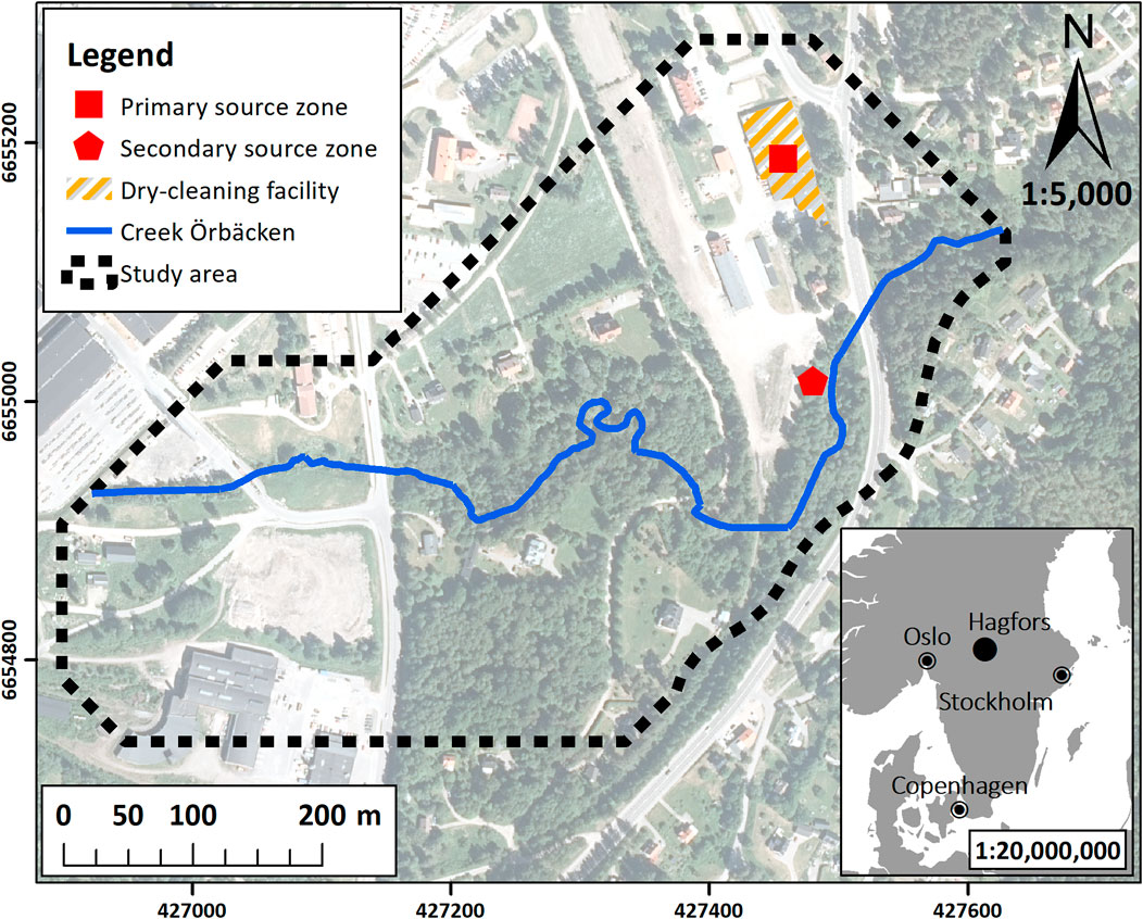
FIGURE 1. Map of the study area showing contamination source zone locations, creek Örbäcken and the extent of the model domain (units are in meters according to the Swedish national reference system, SWEREF99TM). The general direction of groundwater flow (and the direction of flow in the creek) is from the northeast towards the southwest.

The site is situated on Geijersholmsåsen, a glaciofluvial deposit superposing crystalline bedrock extending in the NE-SW direction. It mainly consists of sand and varies between 10 and 30 m in thickness (Gustafsson, 2017). Depth to the water table varies from approximately 12 m near the source zones, to less than 1 m south of the site where a ravine cuts through the sediment. The aquifer is considered unconfined in the study area and transitioning into partially confined near Lake Värmullen where silt and clay covers coarser sediment. Creek Örbäcken, approximately 4 m wide and half a meter deep, flows through a drainage canal around the site from the north to east, before flowing into the ravine south of the site. Here, in the transition zone between two vertically stacked hydrogeological units, a natural degradation zone is located (Åkesson et al., 2021). The creek eventually feeds into Lake Värmullen c. one and a half kilometers west of the site. Earlier investigations have shown PCE concentrations exceeding Swedish drinking water guidelines values (of 10 μg/L, Swedish National Food Agency, 2001) in samples collected from the creek adjacent to the site and down towards the mouth of the lake (Nilsen, 2013).

Since the contaminant was discovered in the 1990s, multiple remediation campaigns of different scale have been undertaken. In 1996, the site was treated using soil vapor extraction, resulting in the removal of 1.5–2 tonnes of PCE from the primary source zone (Nilsen, 2003). Between 2003 and 2004, the site was treated using thermal remediation (steam injection treatment), resulting in the removal of an additional 5 tonnes of PCE from the primary source zone (Nilsen, 2003; Nilsen and Jepsen, 2005). Although large quantities had by then been removed, Nilsen (2013) estimated that there still remained between 20 and 30 tonnes of PCE in the primary source zone, and an additional 10 tonnes of PCE in the secondary source zone.

Creek Örbäcken (the creek) is the primary source of exposure to PCE for people in the area, as it flows through a sparsely populated area. It is also a conduit for rapid transport of PCE to Lake Värmullen. No drinking water wells are known within the area. In 2015, SGU changed the strategic objective from primary source zone treatment to mitigating influx of PCE to the creek (Larsson, 2020a). Yearly PCE mass influx to the creek has previously been estimated to 130 kg using control plane based calculation (Nilsen, 2013) and to 121 kg by computing the arithmetic mean of surface water concentrations multiplied by streamflow rates sampled and measured from December 2018 to February 2020 (Larsson, 2020b). In 2018 and 2019, in situ pilot nano zero-valent iron (nZVI) injection tests were performed in the plume emanating from the primary source zone, approximately 300 m southwest of its source (Larsson, 2021). The purpose was to evaluate the potential of a permeable reactive barrier solution for mitigating groundwater influx to the stream. Unfortunately, results of the campaign indicated no reduction of PCE.

2.1 Previous modelling work of the site

Prior to the remediation efforts presented above, a number of site investigations were performed. As part of the investigative work, to date three different environmental models have been developed.

Andersson (2012), developed a three-dimensional steady-state model in order to ‘study flow patterns within different parts of the groundwater reservoir and to get a better idea of flows and transport times to the surface water recipient’ (creek Örbäcken). The model was developed using Visual Modflow 2011.1, a graphical user interface (GUI) to MODFLOW, and consisted of thirteen hydraulic conductivity (K) zones across four layers. The river (RIV) package was used to calculate SW-GW exchange fluxes in seven zones along the creek, and particle tracking was used to estimate advective transport times from both source zones to the creek. The results indicated a loss of c. 262 m³ per day in groundwater recharge in the upstream section of the creek, and a gain of c. 879 m³ per day in groundwater discharge in the downstream section. Transport times were estimated to between 250–400 days from the primary source zone and c. 60 days from the secondary source zone. The model was history matched using manual regularization (i.e., “trial and error”) by means of adjusting K in the thirteen zones. However, at least five history-matching targets were omitted due to poor fit with field-data in locations of complex geology (Andersson, 2012). Andersson (2012) noted that the model suffered from numerical instability and suggested that a smaller model with higher resolution could improve the fit to data around the area of complex geology. Predictive uncertainties were not explored.

Havn (2018) developed two steady-state MODFLOW models of the site; a ‘homogenous’ and a ‘heterogeneous’ version, using the GMS 10.3 GUI. The reason for developing a homogeneous model was to ‘understand the overall picture of the catchment’ (Havn, 2018). To facilitate visualization in three dimensions, it was constructed using eight homogenous layers. The heterogeneous model consisted of sixteen layers and was developed to ‘simulate and estimate pollution’ from the site. It consisted of five adjustable parameters, including hydraulic conductivity (assigned on a layer-by-layer basis) and stream conductance. Both versions of the model were subject to history matching using two approaches; manual regularization and ‘automated calibration’ (Havn, 2018) using the PEST software. Both approaches, however, lead to large residuals (hydraulic head error exceeding 1.5 m) considering the size of the study area and density of available data. Nevertheless, a solute transport model was developed to run using results from the flow model. Havn (2018) concluded that the model was not able to quantify the scale of pollution and suggested that a higher model resolution could lead to improvements in model capability. A parameter sensitivity analysis was conducted, but predictive uncertainties were not explored.

Korsgaard (2018) developed a 2-dimensional steady-state model using the GUI Visual Modflow Premium 4.6 Classic. The numerical model was discretized as a 100-m-long cross section along the plume emanating from the secondary source zone, reaching across the creek. The primary purpose of the model was to test different remediation scenarios for reducing flux of contaminated groundwater into the creek, including “dig-and-dump” and “pump-and-treat”. A secondary purpose was to estimate the daily volume of contaminated groundwater expected to be collected for remediation treatment. The model consisted of 26 layers with local refinement near the creek. The layers were divided into five K-zones subject to manual parameter adjustment. Seven remediation scenarios were evaluated using groundwater flow-, particle tracking and solute transport simulation. However, no history-matching was performed, and predictive uncertainties were not explored.

3 Model scope

To provide decision makers with information relevant to the current CSM-objective (mitigation of contaminated discharge to the creek), a numerical model was developed to explore SW-GW exchange behavior in the study area (Figure 1). After considering available observation data and computing power, a subjective decision was made to limit the studied period to between the years 2016–2020. To capture seasonal variability in SW-GW exchange fluxes, we choose to history-match field data and simulate SW-GW exchange fluxes under transient conditions. To provide decision makers with as much detail as the selected approach is capable of delivering, the prediction of interest is cell-by-cell SW-GW exchange fluxes on a weekly temporal resolution during the studied period. To increase data assimilation capability, and to reduce risk of numerical instability, we opt for a single-layer model designed around parametrical complexity rather than around structural complexity. This way, parametrical heterogeneity may form as needed, and the model run-time is kept low, which is desirable in a history-matching context (Doherty and Moore, 2020; Hugman and Doherty, 2021). To reduce and quantify predictive uncertainties, we leverage tools of the PEST (Doherty, 2020a) and PEST++ (White, 2018) software suites.

The model architecture and workflow is described in further detail below.

4 Materials and methods

The data used in this study was collected on site as well as downloaded from Swedish authority databases. Streamflow measurements, stream stage measurements, fiber-optic distributed temperature sensing (FO-DTS) and the bulk of hydraulic head measurements were collected by environmental consultant firms Nirás AB (Sebök, 2016; Larsson, 2017; Larsson, 2020b) and Sweco AB (Nilsen, 2013) and supplied to the MIRACHL research group on behalf of SGU. Complementary measurements were collected by the MIRACHL research group during two fieldwork campaigns in the springs of 2017 (see Åkesson et al., 2021) and 2019. Where needed, previously georeferenced data was converted to conform to the Swedish national reference system SWEREF99TM.

Preprocessing of data and model development was performed using the Jupyter Notebook interactive computing platform (Kluyver et al., 2016), following a recent example by White et al. (2020b) on facilitating model reproducibility. The notebooks, which include the work up until the point of history-matching, can be accessed from a Github repository (see Data Availability Statement).

The datasets used in the study are now presented below, followed by a description of the model architecture, model development and history-matching process.

4.1 Datasets and data preparation

Geospatial point cloud data of two types; Lidar and borehole logs, were used to define the spatial extent and topography of the upper and lower model boundary. Because the Lidar data (Lantmäteriet, 2016) was sampled using a relatively high resolution (2x2 m cell size), the dataset was curated to avoid propagating misleading altitudes at bridge crossings before being interpolated to the model grid.

Borehole data collected at the site (Nilsen, 2013; Larsson, 2017) with confirmed or assumed contact with crystalline bedrock, as well as regional borehole data downloaded from the SGU Wells Archive (SGU, 2015) was used to interpolate the extent of the lower model surface.

Daily precipitation data for the Gustavsfors A weather station, located approximately 15 km northeast of Hagfors, was downloaded from the SMHI Open Data Database (SMHI, 2021). Monthly computed evapotranspiration was downloaded for SMHI catchment area 64808 (eastern Hagfors) using the S-HYPE application (Strömqvist et al., 2012), and curated into mean daily evapotranspiration.

Hydraulic head measurements were collected from 63 single- and multilevel wells across the site using both piezometers and manual level meters (Larsson, 2020b). Measurements sampled using piezometers were typically recorded every fourth hour and was resampled into daily averages.

Stream stage, as well as the difference between groundwater head and stream stage (head-stage differences), were measured at five locations along the creek. Measurements were collected using a dual piezometer system where a primary piezometer was installed inside a monitoring well recording the groundwater level, and a secondary piezometer was installed on the outside of the monitoring well recording surface water hydraulic pressure (Larsson, 2017; Larsson, 2020b).

Streamflow was recorded in two different gages located approximately 40 m apart. Data collected with Gage-1 spans the full studied period (2016–2020). However, because streamflow recorded by Gage-1 was suspected to be affected by uncertainties inherent in the sampling methodology, a second gage (Gage-2) was installed in 2018 (Larsson, 2020b).

Fiber-optic distributed temperature sensing (FO-DTS) was used to measure surface water temperatures along three sections of the creek in December 2015 (Sebök, 2016). The discrepancy between surface water-groundwater temperatures were approximately 5 °C, and three warm-water anomalies were detected, indicating influx of groundwater at these positions.

Locations were hydraulic head, stream stage, streamflow and FO-DTS measurements were collected are shown on Figure 2.

FIGURE 2

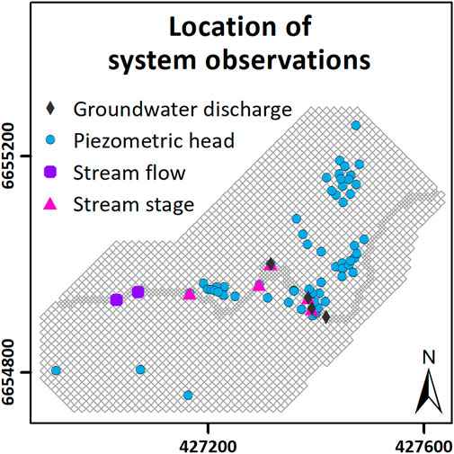
FIGURE 2. Map showing numerical model grid and type and location of history-matching targets. The model grid is refined near monitoring wells and the creek (units are in meters according to the Swedish national reference system, SWEREF99TM).

4.2 Model architecture and development

The model employed in this study is a composite model (the model), consisting of preprocessing software, numerical solvers and postprocessing software open to the public domain. In addition, complementary preprocessing scripts were developed (see 4.2.1) in order to improve site-specific history-matching capability. Model settings, input files and scripts were written and prepared using the Jupyter Notebook environment.

Groundwater flow is simulated with MODFLOW6 (MF6) (Langevin et al., 2022). The MF6 model has a single layer with local refinement around streams and monitoring wells. The model has two stress periods. The first stress period is a steady-state period implemented to acquire representative heads, stream stages and streamflow rates for the beginning of the second stress period; a transient period ranging from December 2015 to December 2019. General head boundaries (GHB) are placed along the boundary of the model domain representing inflows (NW), outflows (SW) and lateral boundaries (SE and NW) of the glaciofluvial aquifer (Figure 3). The Streamflow Routing (SFR) package of MF6 was used to simulate streamflow, stream stage and surface water-groundwater exchange flux in the creek. Setup and configuration of MF6 and its input packages was performed using the python package Flopy (Bakker et al., 2016).

FIGURE 3

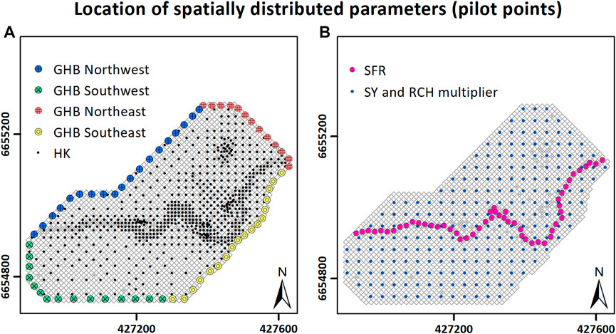
FIGURE 3. Maps showing pilot-point locations of (A) the general head boundaries (GHB) and hydraulic conductivity (HK) and (B), parameters associated with the streamflow routing (SFR) package, specific yield (SY) and groundwater recharge (RCH) multiplier. Units are in meters according to the Swedish national reference system, SWEREF99TM.

Five instances of the lumped parameter recharge model, LUMPREM2 (Doherty J., 2021), were prepared using the python package Lumpyrem (Hugman, 2021), based on daily rainfall and evapotranspiration data presented above (4.1). One instance was used to compute groundwater recharge for use as input by the MF6 Recharge package (RCH). The remaining instances were used to compute time-varying boundary head elevation to the GHBs.

The model architecture is illustrated in Figure 4.

FIGURE 4

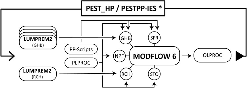
FIGURE 4. Flowchart showing the composite model architecture and flow of information during history-matching (* and uncertainty quantification using PESTPP-IES). The acronyms GHB, SFR, NPF, RCH and STO refer to the MF6 packages General-Head Boundary, Streamflow Routing, Node Property Flow, Recharge, and Storage.

4.2.1 Model parameterization

The model is parameterized using 1709 adjustable parameter values. Pilot points were used to allow spatial variation of physical parameters (Figure 3), including hydraulic conductivity, specific yield, boundary conductance, and spatial variables of the SFR package representing the creek. Hydraulic conductivity pilot points were placed with higher density near the creek and around monitoring wells where the model grid is refined. Covariance matrices taking pilot point density into consideration were created using the PPCOV_SVA and MKPPSTAT utilities (Doherty, 2020b) of the PEST suite. They were applied to constrain parameter covariance and encourage PEST to spread parameter heterogeneity. A temporal covariance matrix was also created for constraining upstream inflow into the starting cell of the SFR package.

During history-matching, writing of parameter values to model input files was done using the model preprocessing software PLPROC (Doherty, 2021c) and three scripts written in the Python language. The three scripts (PP-Scripts in Figure 4) were developed to complement functionality difficult to implement through PLPROC for writing parameter values to the SFR and GHB package of MF6.

4.2.2 Observation targets and feature engineering

History-matching targets include measurements of hydraulic head, streamflow and stream stage collected during the studied period. OLPROC (Doherty, 2021b) was used to time-interpolate model outputs to field measurement time. In addition, OLPROC was also used to feature-engineer existing datasets into datasets of temporal measurement differences for use as observations. Inequality observations (also known as “one-way observations”) (Doherty, 2020a; White et al., 2020a) were used in this study to inform PEST of groundwater influx into the creek at four locations indicated by thermal anomalies in FO-DTS data. Inequality observations were also used to inform PEST that all cells belonging to the SFR-package (which is used to represent the creek) should have an outflow between each cell and its downstream neighbor cell (i.e., the creek should never dry out).

In total 172,059 observations, divided into 15 groups, were used as history-matching targets. Weights were assigned with equal importance to each type of observation during calibration with PEST_HP (Doherty, 2020a). For uncertainty quantification with PESTPP-IES (White, 2018), realizations of measurement noise were generated by changing observation weights to reflect the inverse of the standard deviation of measurement noise for each observation group.

4.2.3 History-matching and uncertainty quantification

History-matching was performed in a three-stage process. First, a standalone instance of the LUMPREM2 model was matched against historical groundwater measurements in a single monitoring well (NI15-O48) using PEST (Doherty, 2018) with Tikhonov (preferred value) regularization. The parameter values that emerged through this process was selected as the initial parameter values of the five LUMPREM2 instances used in the composite model. Secondly, the composite model was history-matched using PEST_HP on Lunarc Aurora, Lund University’s high performance computing (HPC) cluster. After eight iterations PEST_HP was terminated using early stopping to reduce risk of overfitting. Finally, the model was redeployed to the HPC to undergo history-matching and uncertainty quantification using PESTPP-IES. The available computing power allowed for a large ensemble (500 realizations) to be generated and used in the uncertainty quantification process. After five iterations no further meaningful reduction of the objective function was recorded. To reduce risk of underestimating predictive uncertainty, model output obtained from the third iteration of history-matching and uncertainty quantification are presented as the results of this study.

4.3 Estimating groundwater PCE discharge

Because the model is instructed to compute streamflow in addition to SW-GW exchange fluxes, we can use measurements of surface water chemistry collected during the studied period to provide estimations of contaminant mass (PCE) influx. In order to estimate the PCE mass influx required for a given sample, we make the following assumptions; 1) groundwater discharge in the study area is the only source of measured PCE in the creek, 2) the difference in streamflow at the sample location between the sample date and model output date is negligible (the temporal discrepancy between model output dates and sample dates vary between 0–4 days), 3) there is no intra-day variability in PCE concentration at the sample location (i.e., the measured concentration is representative for the full sample date), and 4) the sampled surface water in a cell, from which we obtain measurements of concentration, will be composed of an unknown ratio of groundwater discharge to surface water from upstream of the sample location.

Streamflow through a model cell representing a sample location in the creek can be described as:

$Q_T=Q_{gw}+Q_{sw}$

where $Q_T$ is the total streamflow, $Q_{gw}$ is streamflow fed by groundwater discharge and $Q_{sw}$ is non-groundwater fed streamflow (all flows are in [m³/d]). Upstream groundwater discharge contributing to the total streamflow through a cell can be calculated as:

$Q_{gw}={\displaystyle \sum _{i=0}^n}{Q}_{gw}^i\left[Q_{gw}^i>0\right]$

where $n$ is the number of upstream cells and $Q_{gw}^i$ is groundwater discharge [m³/d] in upstream cells with positive discharge. The index begins at zero to include discharge occurring in the cell representing the sample location. The ratio of groundwater discharge to total streamflow is given by:

$Q_{gw}^r=\frac{Q_{gw}}{Q_T}$

As groundwater is discharged into the creek, the groundwater PCE concentrations are diluted by surface water. Using the ratio of groundwater discharge to total streamflow ($Q_{gw}^r$), we can infer the concentration of PCE in upstream groundwater discharge required for a given surface water sample:

$C_{gw}=\frac{C_M}{Q_{gw}^r}$

where $C_{gw}$ is the concentration of the upstream groundwater discharge and $C_M$ is the measured concentration of the water sample (concentrations are in [kg/m³]). Using the concentration of the upstream groundwater discharge ($C_{gw}$), we can infer the mass of PCE [kg] discharged into the stream for a given surface water sample:

${PCE}_m=Q_{gw}\bullet C_{gw}$

By calculating ${PCE}_m$ for each member of the model ensemble, the prior and posterior uncertainty in streamflow and SW-GW exchange fluxes is taken into consideration and a probabilistic estimation of the PCE influx is provided. There are 631 surface water chemistry samples collected from different locations in the creek during the studied period for which a PCE-influx estimation is provided.

5 Results

5.1 Simulated SW-GW exchange fluxes

The model was instructed to calculate SW-GW exchange fluxes once per week during the studied period (2016–2020). Of the 500 initial realizations, 485 realizations resulted in convergence. History-matching reduced uncertainties in simulated SW-GW exchange fluxes in all sections of the creek. Upon inspecting a posteriori model results, we have divided the creek into twelve reaches (segments), based on their SW-GW exchange behavior, as shown in Figure 5. Predictive uncertainties remain fairly high in the first reach, but decrease significantly in the second reach, which is located adjacent to monitoring wells from which data was included as history-matching targets. Predictive uncertainties also remain fairly high in reaches eight and nine, which represents the final part of a small meander bend.

FIGURE 5

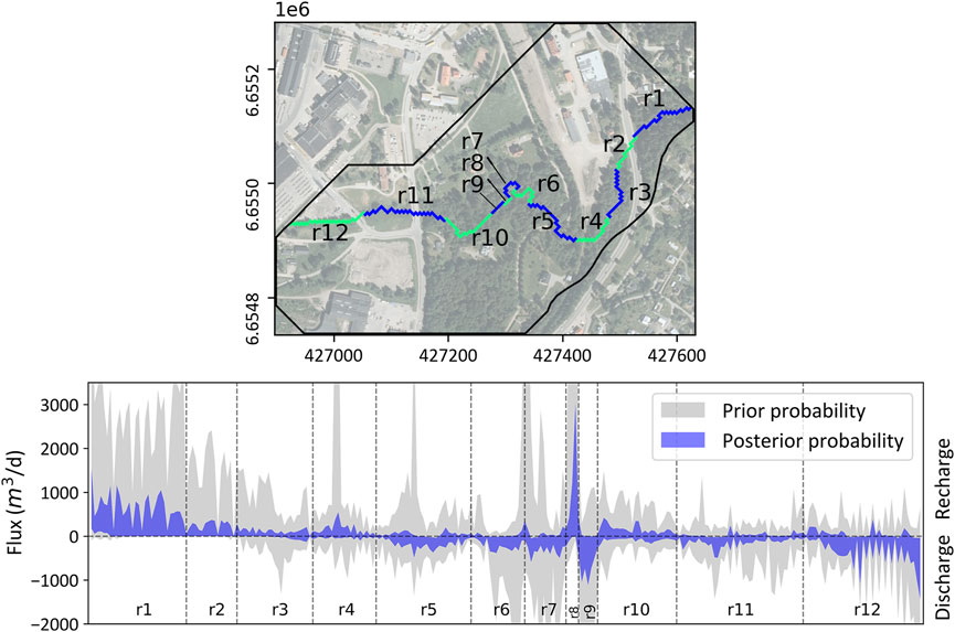
FIGURE 5. Prior and posterior SW-GW exchange flux uncertainty. The creek is divided into reaches (segments) based on SW-GW exchange behavior. Map units are in meters according to the Swedish national reference system, SWEREF99TM.

In general, the creek is contributing to groundwater recharge in the first four reaches. Mean simulated recharge in this section is calculated to c. 7204 m³/d but is associated with a considerable variability during the studied period (σ ≈ 3070 m3/d). Reaches five through seven represent three segments where groundwater is discharged to the creek. Mean simulated discharge in this section is calculated to c. 3102 m3/d (σ ≈ 1679 m3/d). In reaches seven through nine, which represent a relatively small meandering section of the creek, the posterior uncertainty remain relatively high. Considered at the mean of the posterior ensemble, this section contribute with a slight mean groundwater discharge of c. 224 m3/d (σ ≈ 608 m3/d). Simulated SW-GW exchange behavior in reach ten is considered neutral with a very small mean groundwater recharge of c. 5 m3/d (σ ≈ 427 m3/d). The final two reaches, reach eleven and twelve, contribute with a mean groundwater discharge of c. 5328 m3/d (σ ≈ 2574 m³/d).

Temporal variability in simulated SW-GW exchange fluxes is shown in Figure 6. Locations where groundwater is recharged from the creek is described as losing conditions, and vice versa. As shown, temporal variability in SW-GW exchange behavior remain fairly static for the studied period. The most pronounced variability can be observed during the months of April and May of 2018 and 2019 in reaches five through twelve, indicating less discharge to the creek compared to the same period of the two preceding years. This is also, in general, the periods where predictive uncertainties pertaining to temporal variability are the highest.

FIGURE 6

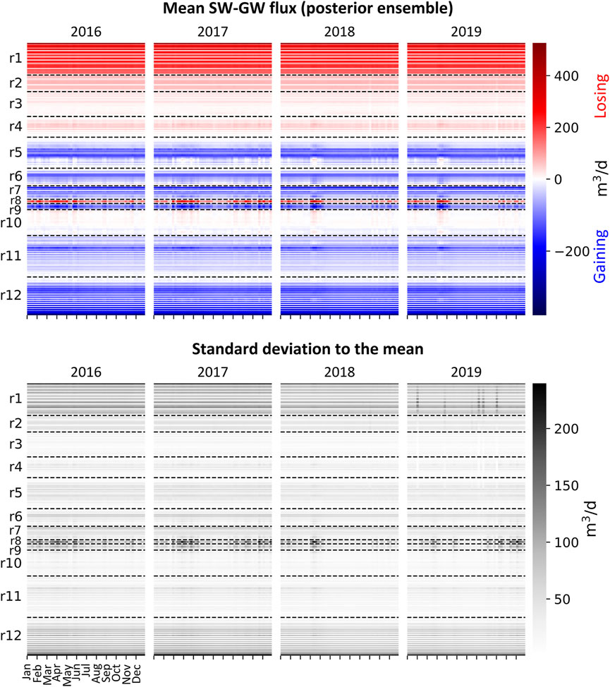
FIGURE 6. Heatmaps showing temporal variability in SW-GW exchange flux during the studied period in weekly output. The upper row (colorized) show mean of the posterior ensemble and the lower (grayscale) row show posterior ensemble standard deviation of the mean.

5.2 PCE mass influx estimation

Using equations 1 to 4, measured concentrations of surface-water PCE was used to infer the groundwater discharge PCE concentrations, for each of the 631 samples. Eq. (5) was then used to compute PCE mass influx by multiplying simulated groundwater discharge with inferred groundwater PCE concentrations. This was done for each member of the model ensembles, resulting in 293,789 computations of prior and posterior daily PCE mass influx estimations respectively. The results are shown in Figure 7, and is color coded by surface water flow regime, which we categorized as low flow (<25th percentile), regular flow (between 25th and 75th percentile) and high flow (>75th percentile). In general, computed upstream PCE influx increase in the downstream direction and is highest during periods of high flow, which can be observed in the upper plot of Figure 7. Locations of influx (groundwater discharge) for the three flow regimes, and their respective uncertainty, is shown on the bottom plot. The computed upstream PCE influx follow a log-normal distribution, with a log₁₀ geometric mean of c. 0.55 kg/d. Uncertainties in computed mass influx are described using the 5th and 95th percentiles and are based on posterior uncertainties in SW-GW exchange fluxes and streamflow, as well as laboratory measurement uncertainties pertaining to the chemistry samples.

FIGURE 7

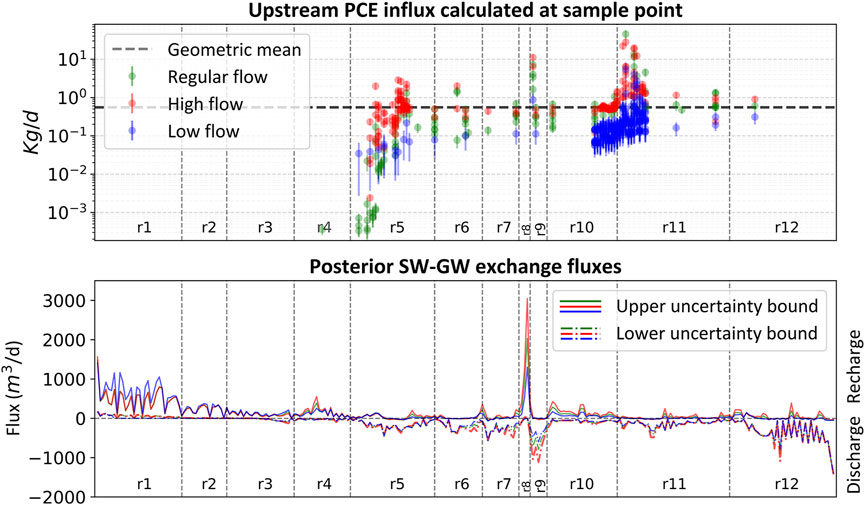
FIGURE 7. Upper plot showing estimated PCE mass influx per sample under regular, high and low streamflow. The geometric mean is 0.55 kg/d. High peaks in mass influx tend to occur in areas characterized by groundwater discharge. Bottom plot showing upper and lower uncertainty bounds of posterior SW-GW exchange fluxes under different flow regimes. Notable differences in predictive uncertainty can be observed in reaches one, eight and nine.

6 Discussion

6.1 Model workflow challenges and opportunities

Challenges arising during construction of the model were mainly associated with the SFR package of MF6. Implementing the SFR package in a history-matching context require extra careful consideration in comparison to many of the commonly used MODFLOW packages. This is because SFR does not allow a parameter known as reach streambed top elevation (rtp) to increase in the downstream direction. If this requirement is not met MODFLOW will return an error and history-matching will be terminated prematurely. In our case, which will likely also be the case for many others utilizing the SFR package, initial rtp values were obtained by sampling a digital elevation map (DEM). However, undulating topography in the DEM yielded invalid input for a portion of the SFR cells. Leaf et al. (2021) created SFRmaker, a Python package designed to automate the workflow of implementing the SFR package and curate valid input. However, at the time of writing this paper, SFRmaker only supports structured grids. Because the model in this study utilizes an unstructured grid, we implemented a solution inspired by SFRmaker to ensure that the requirement described above is met:

$\left|{rtp}_i\right|=\left\{\begin{array}{c}{x}_i,ifi=1\\ x_i,if{x}_i<x_{i-1}\\ x_{i-1},if{x}_i\ge x_{i-1}\end{array}\right.$

where $x_i$ is the sampled elevation at the center point of the $i$-th cell of the SFR package.

Another potential issue related to the SFR package in the context of history-matching is the drying out of streamflow cells. During early iterations, we discovered that PEST_HP sought solutions of minimum error variance that included dry streamflow cells for small parts of the creek. Because we know from extensive site investigation, as well as from measured data, that the creek does not dry out, this presented a problem. In order to address this issue, we implemented inequality observations to instruct PEST_HP and PESTPP-IES to seek solutions where the streamflow between a cell and its downstream neighbor was positive.

Fiber-optic distributed temperature sensing (FO-DTS) data presents an interesting opportunity in terms of data assimilation. To the best of our knowledge, this is the first time FO-DTS thermal anomalies are used in the context of history-matching. In order for groundwater discharge to be detected as a thermal anomaly in FO-DTS data, groundwater and surface water must be of different temperatures. Because of this, usability of FO-DTS may vary according to site and season. In addition, length of the FO cable presents a practical constraint on its usability, making it better suited for use in models representing smaller sites. In this study, thermal anomalies were implemented in the form of inequality observations of groundwater discharge, meaning that PEST considers the residual of an observation as zero when discharge is greater than 0 m³/d. Future work where thermal anomalies are assimilated during history-matching could explore the use of less conservative inequality constraints, or, even the use of thermal anomalies as regular, numerical observations. Longer time series would also facilitate studies on data worth under a variety of predictions where SW-GW interaction play a role.

6.2 Simulated SW-GW exchange fluxes and estimations of PCE mass influx

Predictive uncertainties pertaining to SW-GW exchange fluxes were reduced significantly as a result of history-matching, enabling high resolution spatiotemporal characterization as shown in Figure 6. Predictive uncertainties remain relatively high in the first and last (12th) reach, as well as in reach eight and nine, located centrally in the study area. Uncertainties pertaining to the first and last reach can likely be explained by the absence of history-matching targets in these sections of the creek. Reaches eight and nine represent the final part of a small meander bend. As shown in the bottom plot of Figure 7, uncertainty in this section is particularly sensitive to variability in streamflow compared to other sections of the creek. One possible cause for this could be the model’s inability to allow for temporal variability of spatial parameters pertaining to the creek. For example, during times of heavy rains and melting snow (conditions that cause high streamflow rates), the stream width is expected to widen as water levels rise and progressively cover the point bar deposits. Although stream width is considered adjustable parameters in this study, it is not configured to allow for temporal variability.

Seasonal variability in SW-GW exchange fluxes is relatively low, with the exception of reaches five through eleven in April and May of 2018 and 2019 (Figure 6). In 2018, northern Europe was affected by an extreme drought that persisted into 2019 (Bakke et al., 2020). This is a plausible explanation for the anomalous behavior in SW-GW exchange fluxes observed in the creek during this period, which indicate greater groundwater recharge and lesser groundwater discharge than normal.

As shown in the upper plot of Figure 7, uncertainty in PCE mass influx is greater during times of low flow. This is because posterior uncertainties in streamflow are greater during periods of low flow (mean coefficient of variation, mCV ≈0.23), compared to periods of regular flow (mCV ≈0.15) or high flow (mCV ≈0.08).

The estimations of PCE mass influx were based on a list of assumptions (4.3). Although we can be fairly certain that the first assumption holds true (no alternative sources to measured PCE other than groundwater discharge in the studied area), the second and third assumptions require discussion. The second assumption, namely, that difference in streamflow between sample date and model output date (varying between zero to 4 days) is negligible is a simplified assumption, as, for example, bursts of heavy rainfall may momentarily impact streamflow rates and levels. The third assumption, that there is no intra-day variability in PCE concentration at the sample locations, also represent a simplified assumption. PCE is a dense non-aqueous phase liquid (DNAPL), a hydrophobic compound known to generate extensive variability in mass discharge (Guilbeault et al., 2005) not only temporally, but also spatially. Larsson (2020b) suggest that incomplete mixing of the surface water in the creek may lead to great variability in measured concentrations depending on whether the sample was collected centrally or near the banks. Both assumptions discussed above are associated with uncertainties that are unquantified pertaining to the mass influx estimations. However, because the samples on which the estimations are based, were collected during periods of varying streamflow, as well as spatially varying along both axes of the creek, it could be argued that the estimations of mass influx, when looked at as a distribution, take this uncertainty somewhat into consideration.

6.3 Earlier studies and new findings

As discussed earlier (2.1), three models were previously developed of this site. Because particle tracking and solute transport modelling was outside the scope of this study, direct comparisons with Havn (2018) and Korsgaard (2018) are difficult to make at this point.

Andersson (2012) discretized the creek into seven zones and calculated total SW-GW exchange fluxes for each zone. Anderson (2012) found that groundwater recharge was occurring in the first zone, and discharge was occurring in the remaining six zones. As we have shown (Figures 5–7), SW-GW exchange behavior in the creek is complex, especially in the meandering sections where spatiotemporal variations can be expected to be large. Therefore, we cannot exclude the possibility of groundwater recharge occurring further downstream if we are to consider the distribution of posterior uncertainty. By selecting a subsection of the creek overlapping the two studies, we found the section of upstream recharge to be significantly longer (c. 28 percent), and more importantly, that SW-GW exchange fluxes were significantly larger than previously estimated (Figure 8, upper row).

FIGURE 8

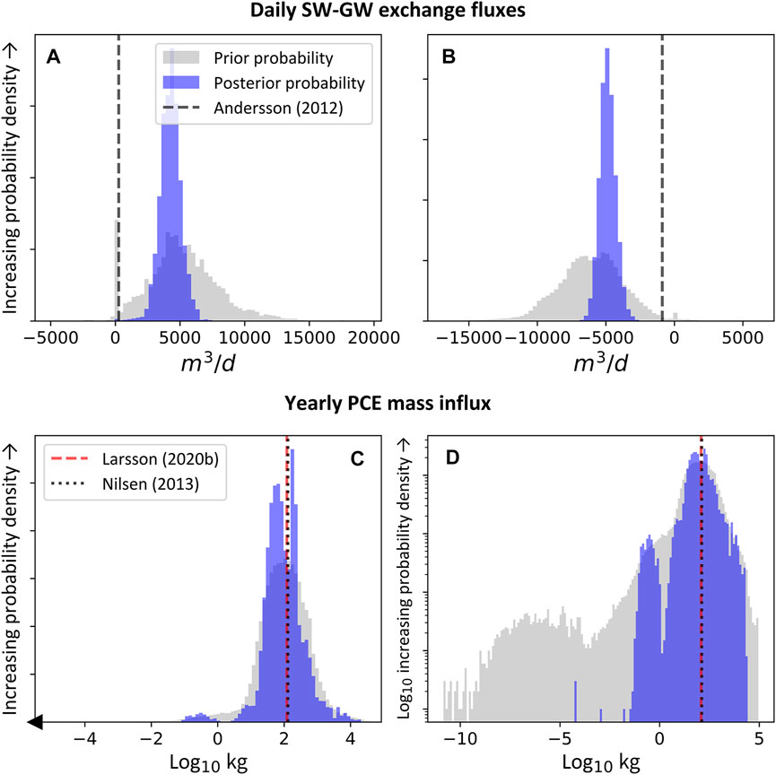
FIGURE 8. Comparisons between results in this study (represented as prior and posterior probability distributions in gray and blue) and results obtained in earlier studies of the Hagfors contaminated site. Upper row showing comparisons with results in Andersson (2012) of (A) simulated SW-GW exchange flux of the upstream section of the creek characterized by recharge (approximately corresponding to reaches two to four), and (B) SW-GW exchange flux of reaches five to eleven characterized by discharge. Bottom row showing comparisons with previous estimates of PCE mass influx where (C) show yearly PCE mass influx using a truncated x-axis to enhance visibility of the posterior probability distribution, and (D) yearly PCE mass influx with a logarithmic y-axis to highlight reduction of predictive uncertainty achieved during history-matching.

Unfortunately, the model was not equally successful in reducing predictive uncertainties pertaining to PCE mass influx. By multiplying results obtained through Equation (5) by 365, we can compare our estimates with prior estimations (Nilsen, 2013; Larsson, 2020b) of mass influx (Figure 8, bottom row) per year. As shown, both prior estimations are located near the center of the posterior probability distribution. Interestingly, we find two peaks in the posterior probability distribution. To determine whether the bimodal distribution was caused by the model or the chemistry input dataset, we tracked each realization (thereby also tracking each set of model parameters) contributing to the results of the left and right peak respectively. However, we found no meaningful variability in model contribution between the two peaks (i.e., all realizations contributed to both peaks). Measured concentrations in the creek, however, appear with a bimodal distribution, and is therefore the only logical contributing factor for the shape of the mass influx estimations as shown on Figure 8. As Larsson (2020b) suggested, incomplete mixing of surface water is a likely explanation for why the surface water chemistry dataset appear bimodal.

Uncertainty in PCE mass influx, as estimated in this study, can originate from uncertainty in streamflow, uncertainty in SW-GW exchange fluxes and in uncertainties related to surface water chemistry measurements. Uncertainties pertaining to the first two origins were reduced significantly during history-matching, but uncertainties related to surface water chemistry persist. Nevertheless, an uncertainty range has been quantified.

7 Conclusion

With the current CSM objective being set on mitigating influx of PCE to creek Örbäcken, a prediction relevant to the objective (characterization of SW-GW exchange fluxes) was selected for this study. The ensuing model workflow and architecture was designed to facilitate data assimilation of prediction pertinent information in historical measurements through history-matching. By adopting a single-layer approach with local refinement near the creek and around monitoring wells for which historical measurements were available, the model run time could be constrained. This was important, because history-matching requires many model runs. We used a highly parameterized model, which allowed for parametrical heterogeneity to evolve where needed during history-matching. In addition to classical types of observations, we also assimilated thermal anomalies in FO-DTS measurements as locations of groundwater discharge, through the use of inequality observations. Challenges pertaining to implementing the SFR package in a history-matching context and suggestions for how to overcome them was discussed. Predictive uncertainties were reduced and explored using the iterative ensemble smoother of the PEST++ suite.

As a result, we were able to characterize SW-GW exchange fluxes in the creek in high spatiotemporal resolution, showing locations of (and quantifying) contaminated groundwater discharge. Seasonal variability pertaining to SW-GW exchange fluxes was found to be low, with the exception of an unusual drought event that occurred during 2018–2019. We also found that SW-GW exchange fluxes are likely to be significantly larger than previously estimated. Using surface water chemistry measurements, we estimated PCE mass influx and found estimations in two earlier studies to be located near the center of the posterior probability distribution. The uncertainty pertaining to PCE mass influx was only reduced slightly, but has now been quantified.

Our recommendation for decision makers, with regards to the current CSM objective, is to focus remediation action toward reaches 5–7, 9, 11 and 12, according to modelling results.

Data availability statement

Modeling workflow up until the point of history-matching is documented in a collection of Jupyter Notebooks. They can be accessed from the following GitHub repository: https://github.com/nikobenho/hagfors_gwm. Requests to access the history-matched model should be directed to nikolas.hoglund@geol.lu.se.

Author contributions

NH, CS, and RH conceived the idea. NH analysed the data. NH (with support and guidance from RH) set up the modelling environment and undertook all simulations and their postprocessing. NH and CS wrote the paper. RH reviewed the manuscript, provided critical feedback and helped shape the research. All authors contributed to the article and approved the submitted version.

Funding

Funding for the work was provided by Formas, The Swedish Research Council for Environment (ref. 2016-20099 and 2016-00808), SBUF (ref. 13336), ÅForsk (ref. 14-332), SGU, NCC, and Sven Tyréns Stiftelse and Lund University.

Acknowledgments

Ulf Winnberg and Kristin Forsberg at SGU is thanked for fruitful discussion concerning site strategy and encouragement. Nicklas Larsson and Gro Lilbæk at Nirás AB is acknowledged for providing data crucial for the implementation and realization of this study. Professor John Doherty (Flinders University, Watermark Numerical Computing) is thanked for providing the Linux version of the PEST suite, as well as for providing compilation instructions. The data handling/computations were enabled by resources provided by the Swedish National Infrastructure for Computing (SNIC) at Aurora and LU Local partially funded by the Swedish Research Council through grant agreement no. 2018-05973. Marcos Acebes at SNIC support is acknowledged for assistance concerning technical and implementation aspects.

Conflict of interest

Author RH was employed by INTERA.

The remaining authors declare that the research was conducted in the absence of any commercial or financial relationships that could be construed as a potential conflict of interest.

Publisher’s note

All claims expressed in this article are solely those of the authors and do not necessarily represent those of their affiliated organizations, or those of the publisher, the editors and the reviewers. Any product that may be evaluated in this article, or claim that may be made by its manufacturer, is not guaranteed or endorsed by the publisher.

References

Åkesson, S., Sparrenbom, C. J., Paul, C. J., Jansson, R., and Holmstrand, H. (2021). Characterizing natural degradation of tetrachloroethene (PCE) using a multidisciplinary approach. Ambio 50. doi:10.1007/s13280-020-01418-5

CrossRef Full Text | Google Scholar

Anderson, M. P. (2005). Heat as a ground water tracer. Groundwater 43, 951–968. doi:10.1111/j.1745-6584.2005.00052.x

CrossRef Full Text | Google Scholar

Andersson, S. (2012). Modellering av grundvattenflöden vid f.d Hagforstvätten med Visual MODFLOW (in Swedish). Report No: 133.1178.000. Karlstad, Sweden: Sweco Environment AB.

Google Scholar

Bakke, S. J., Ionita, M., and Tallaksen, L, M. (2020). The 2018 northern European hydrological drought and its drivers in a historical perspective. Hydrology Earth Syst. Sci. 24, 5621–5653. doi:10.5194/hess-2020-239

CrossRef Full Text | Google Scholar

Bakker, M., Post, V., Langevin, C. D., Hughes, J. D., White, J. T., Starn, J. J., et al. (2016). Scripting MODFLOW model development using Python and FloPy. Groundwater 54, 733–739. doi:10.1111/gwat.12413

CrossRef Full Text | Google Scholar

Barul, C., Fayossé, A., Carton, M., Pilorget, C., Woronoff, A-S., Stücker, I., et al. (2017). Occupational exposure to chlorinated solvents and risk of head and neck cancer in men: A population-based case-control study in France. Environ. Health 16, 77. doi:10.1186/s12940-017-0286-5

PubMed Abstract | CrossRef Full Text | Google Scholar

Briggs, M. A., Lautz, L. K., and McKenzie, J. M. (2012). A comparison of fibre-optic distributed temperature sensing to traditional methods of evaluating groundwater inflow to streams. Hydrol. Process. 26, 1277–1290. doi:10.1002/hyp.8200

CrossRef Full Text | Google Scholar

Caers, Jef. (2011). Modeling uncertainty in the Earth sciences. Chichester, UK: John Wiley and Sons.

Google Scholar

Chapman, S. W., Parker, B. L., Cherry, J. A., Aravena, R., and Hunkeler, D. (2007). Groundwater–surface water interaction and its role on TCE groundwater plume attenuation. J. Contam. Hydrology 91, 203–232. doi:10.1016/j.jconhyd.2006.10.006

CrossRef Full Text | Google Scholar

Cook, P. G. (2013). Estimating groundwater discharge to rivers from river chemistry surveys: Groundwater discharge to rivers. Hydrol. Process. 27, 3694–3707. doi:10.1002/hyp.9493

CrossRef Full Text | Google Scholar

Doherty, J. E. (2021c). PLPROC – a parameter list processor. Brisbane: Watermark Numerical Computing.

Google Scholar

Doherty, J. E. (2020b). Groundwater data utilities – Part B: Program descriptions. Brisbane: Watermark Numerical Computing.

Google Scholar

Doherty, J. E. (2021b). OLPROC – an observation list processor for use with PEST and PEST++. Brisbane: Watermark Numerical Computing.

Google Scholar

Doherty, J. E. (2018). Pest – model-independent parameter estimation – user manual Part 1: PEST, SENSAN and global optimisers. Brisbane: Watermark Numerical Computing.

Google Scholar

Doherty, J. E. (2020a). PEST_HP – PEST for highly parallelized computing environments. Brisbane: Watermark Numerical Computing.

Google Scholar

Doherty, J., and Simmons, C. T. (2013). Groundwater modelling in decision support: Reflections on a unified conceptual framework. Hydrogeol. J. 21, 1531–1537. doi:10.1007/s10040-013-1027-7

CrossRef Full Text | Google Scholar

Doherty, J. (2021a). Version 2 of the LUMPREM groundwater recharge model. Brisbane: Watermark Numerical Computing.

Google Scholar

Guha, N., Loomis, D., Grosse, Y., Lauby-Secretan, B., El Ghissassi, F., Bouvard, V., et al. (2012). Carcinogenicity of trichloroethylene, tetrachloroethylene, some other chlorinated solvents, and their metabolites. Lancet Oncol. 13, 1192–1193. doi:10.1016/s1470-2045(12)70485-0

PubMed Abstract | CrossRef Full Text | Google Scholar

Guilbeault, M. A., Parker, L. B., and Cherry, J. A. (2005). Mass and flux distributions from DNAPL zones in sandy aquifers. Groundwater 43, 70–86. doi:10.1111/j.1745-6584.2005.tb02287.x

CrossRef Full Text | Google Scholar

Gustafsson, M. (2017). Grundvattenmagasinet Hagfors (in Swedish). Report No. 250 500 029. Uppsala, Sweden: Sveriges Geologiska Undersökning SGU.

Google Scholar

Havn, H. H. (2018). Master’s thesis. Copenhagen, Denmark: Copenhagen University. Groundwater flow and transport of chlorinated solvents at Hagfors, Sweden: Modelling historic impact and possible remediation of pollution of Örbäcken Creek

Google Scholar

Hugman, R. (2021). Lumpyrem. Available at: https://github.com/rhugman/lumpyrem.

Google Scholar

Kluyver, T., Ragan-Kelley, B., Pérez, F., Granger, B., Bussonnier, M., Frederic, J., et al. (2016). “Jupyter notebooks – A publishing format for reproducible computational workflows,” in Positioning and power in academic publishing: Players, agents and agendas. Editors Fernando Loizides, and Birgit Scmidt (Göttingen, Germany: IOS Press).

Google Scholar

Korsgaard, A. (2018). Hagforstvätten. Uppställning av och beräkning med grundvattenmodell (in Swedish). Report No. 215147-22. Malmö, Sweden: NIRÁS.

Google Scholar

Langevin, C. D., Hughes, J. D., Banta, E. R., Provost, A. M., and Panday, S. (2022). MODFLOW 6 modular hydrologic model. Reston, Virginia, USA: United States Geological Survey.

Google Scholar

Lantmäteriet, (Swedish mapping, cadastral and land registration authority) (2016). GSD-Höjddata, 608 grid 2+. Available at: https://maps.slu.se/get/ (Accessed May 21, 2021).

Google Scholar

Larsson, N. (2020a). F.d. FFV tvätteri Hagfors – handlingsplan. Malmö, Sweden: NIRÀS.

Google Scholar

Larsson, N. (2021). Hagforstvätten Pilotförsök – resultat av miljökontroll vid permeabel reaktiv barriär i utströmningsområde 3 (in Swedish). Project No. 32400316-010. Malmö, Sweden: NIRÀS.

Google Scholar

Larsson, N. (2020b). Hagforstvätten – justering av miljökontrollprogram för Örbäcken. Malmö, Sweden: NIRÀS.

Google Scholar

Larsson, N. (2017). Project No. 5000515. Sweden: Malmö: NIRÁS. Hagforstvätten – resultatrapport från undersökningar dec 2013 – jan 2017 (in Swedish)

Google Scholar

Leaf, A. T., Fienen, M. N., and Reeves, H. W. (2021). SFRmaker and linesink-maker: Rapid construction of streamflow routing networks from hydrography data. Groundwater 59, 761–771. doi:10.1111/gwat.13095

CrossRef Full Text | Google Scholar

Nickels, J. L., Genereux, D. P., and Knappe, D. R. U. (2023). Improved Darcian streambed measurements to quantify flux and mass discharge of volatile organic compounds from a contaminated aquifer to an urban stream. Journal of Contaminant Hydrology 253, 104124. doi:10.1016/j.jconhyd.2022.104124

PubMed Abstract | CrossRef Full Text | Google Scholar

Nilsen, J. (2013). Hagforstvätten, huvudstudie (in Sweden). Report No. 133.1178 000. Karlstad, Sweden: Sweco Environment AB

Google Scholar

Nilsen, J. (2003). Hagforstvätten. Lägesrapport kall sanering av perkloretylen (in Swedish). Report No. 154.4157 000. Karlstad, Sweden: Sweco VBB AB.

Google Scholar

Nilsen, J., and Jepsen, J. D. (2005). Hagforstvätten. Termisk insitu-sanering av perkloretylen, avslutande rapport (in Swedish). Report No. 233.4157 000. Karlstad, Sweden: Sweco VBB AB.

Google Scholar

Ntona, M. M., Busico, G., Mastrocicco, M., and Kazakis, N. (2022). Modeling groundwater and surface water interaction: An overview of current status and future challenges. Sci. Total Environ. 846, 157355. doi:10.1016/j.scitotenv.2022.157355

PubMed Abstract | CrossRef Full Text | Google Scholar

Pankow, J. F., and Cherry, J. A. (1996). Dense chlorinated solvents and other DNAPLs in groundwater: History, behavior, and remediation. Portland, Oregon: Waterloo Press.

Google Scholar

Partington, D., Knowling, M. J., Simmons, C. T., Cook, P. G., Xie, Y., Iwanaga, T., et al. (2020). Worth of hydraulic and water chemistry observation data in terms of the reliability of surface water-groundwater exchange flux predictions under varied flow conditions. J. Hydrology 590, 125441. doi:10.1016/j.jhydrol.2020.125441

CrossRef Full Text | Google Scholar

Schilling, O. S., Cook, P. G., and Brunner, P. (2019). Beyond classical observations in hydrogeology: The advantages of including exchange flux, temperature, tracer concentration, residence time, and soil moisture observations in groundwater model calibration. Rev. Geophys. 57, 146–182. doi:10.1029/2018RG000619

CrossRef Full Text | Google Scholar

Schmoll, O., Howard, G., Chilton, J., and Chorus, I. (2006). Protecting groundwater for health: Managing the quality of drinking-water sources. London, UK: IWA Publishing.

Google Scholar

Sebök, E. (2016). Temperaturmålinger i Örbäcken, Hagfors, Sverige (in Danish).

Google Scholar

Selker, J. S., The´venaz, L., Huwald, H., Mallet, A., Luxemburg, W., van de Giesen, N., et al. (2006). Distributed fiber-optic temperature sensing for hydrologic systems. Water Resour. Res. 42, W12202. doi:10.1029/2006WR005326

CrossRef Full Text | Google Scholar

SEPA (Swedish Environmental Protection Agency), (2007). Klorerade lösningsmedel – identifiering och val av efterbehandlingsmetod (in Swedish). Report No. 5663. Stockholm, Sweden: Naturvårdsverket

Google Scholar

SMHI, (2021). Weather station data for Gustavsfors A. Available at: https://www.smhi.se/data/meteorologi/ladda-ner-meteorologiska-observationer/.

Google Scholar

Strömqvist, J., Arheimer, B., Dahné, J., Donnelly, C., and Lindström, G. (2012). Water and nutrient predictions in ungauged basins: Set-up and evaluation of a model at the national scale. Hydrological Sci. J. 57, 229–247. doi:10.1080/02626667.2011.637497

CrossRef Full Text | Google Scholar

Swedish National Food Agency, (2001). Slvfs 2001:30: The Swedish National Food Agency’s regulations on drinking water. Stockholm, Sweden: Swedish National Food Agency.

Google Scholar

White, J. T. (2018). A model-independent iterative ensemble smoother for efficient history-matching and uncertainty quantification in very high dimensions. Environ. Model. Softw. 109, 191–201. doi:10.1016/j.envsoft.2018.06.009

CrossRef Full Text | Google Scholar

White, J. T., Foster, L. K., Fienen, M. N., Knowling, M. J., Hemmings, B., and Winterle, J. R. (2020a). Toward reproducible environmental modeling for decision support: A worked example. Front. Earth Sci. 8. doi:10.3389/feart.2020.00050

CrossRef Full Text | Google Scholar

White, J. T., Hunt, R. J., Fienen, M. N., and Doherty, J. E. (2020b). Approaches to highly parameterized inversion: PEST++ version 5, a software suite for parameter estimation, uncertainty analysis, management optimization and sensitivity analysis. U.S. Geol. Surv. Tech. Methods 7C26. doi:10.3133/tm7c26

CrossRef Full Text | Google Scholar

Woessner, W. W. (2020). Groundwater-surface water exchange. Ontario, Canada: The Groundwater Project.

Google Scholar

Wöhling, T., Gosses, M. J., Wilson, S. R., and Davidson, P. (2018). Quantifying River-groundwater interactions of New Zealand's gravel-bed rivers: The wairau plain. Groundwater 54, 647–666. doi:10.1111/gwat.12625

CrossRef Full Text | Google Scholar