1 Introduction
The electromagnetic induction method is an important branch of geophysical-electrical exploration, which mainly uses the differences in electrical conductivity, permeability and dielectricity of the subsurface medium and applies the principle of electromagnetic induction to observe and study the distribution patterns (frequency characteristics and temporal characteristics) of artificial or naturally occurring electromagnetic fields and thus solve relevant geological problems (Tikhonov, 1950; Cagniard, 1953; He, 2010a; He, 2019; Chen et al, 2014a). Therefore, studying the frequency response of the earth to electromagnetic fields can obtain the distribution pattern of the resistivity of the subsurface medium at different depths (Zonge, 1991; He, 2019; He, 2020; Liu et al, 2019; Liu et al, 2022; Li et al, 2023). In electrical exploration, the electromagnetic field itself has interference and resonance phenomena, which complicates the characteristics of the field. By introducing an appropriate definition of apparent resistivity, highlighting the useful information and suppressing the interference information can help us make good analysis and judgment of the observation results, which is beneficial to the inverse interpretation, so the study of the definition of apparent resistivity is meaningful (Yin et al, 1991a; Liu et al, 2013; Chen, 2014b).
There are several resistivity definition methods in the frequency domain EM method, which are mostly based on the uniform half-space model (Spies, 1986; Yin et al, 1991b; Tang et al, 2005). ТИxohob (1950) and Cagniard (1953) separately and independently proposed the Magnetotelluric (MT), which defined the apparent resistivity by a pair of orthogonal component electric field to magnetic field ratios, and established the apparent resistivity as the interpretation parameter. Goldstein (1971) proposed controlled source audio Magnetotelluric method (CSAMT), which replaced natural source with a controlled source. However, there is a complex implicit function relationship between the uniform half-space surface electromagnetic field values and resistivity in the controlled source frequency domain electromagnetic method, and it is difficult to find the explicit inverse function between resistivity and field by analytical methods (He, 2010a; Li et al, 2013), Therefore, the complex high-order function in the field is abandoned, and the MT method is used to define the apparent resistivity parameter. Therefore, the near zone, mid-zone, and wave zone were divided according to the variation properties of the electromagnetic field (Yin et al, 1991a; Liu et al, 2013), and the approximate definition of the apparent resistivity in the wave zone was adopted, resulting in serious distortion of the apparent resistivity in the mid-zone and near zone, which affects the interpretation of the sounding curve (Yin et al, 1991b; Liu et al, 2013; Cheng et al, 2014b; Tang et al, 1994; Tang, 1993).
In order to unify the wave zone, mid-zone and near zone, a full-zone apparent resistivity is defined, which can reflect the vertical electrical variation of the geoelectric section directly and also expand the controlled source observation zone (Cao, 1978; Huang et al, 1992; Tang et al, 1993; Tang et al, 1994). Yin et al (1991a) pointed out that the definition of full-zone apparent resistivity can reflect information of the geoelectric section more realistically than other approximate definitions and is less influenced by the pole distance. Fang et al (1992) compared the exact formula of uniform half-space field with the formula of the wave zone to obtain a correction coefficient K, and multiplied the apparent resistivity defined in the wave zone by the correction coefficient K to obtain the apparent resistivity value defined in the full zone. This method is simple and easy to implement. Mao and Bao (1996) proposed a direct algorithm for the full-zone apparent resistivity, which is a concise and accurate method. Tang and He (2005) analyzed and compared in detail the differences and similarities of apparent resistivity defined by wave zone and full zone. He (2010b) proposed the wide field electromagnetic sounding method based on the analytic expressions of electromagnetic fields of horizontal current sources and vertical magnetic sources at the ground in semi-uniform space, and proposed the use of computers to realize the calculation of wide field apparent resistivity using the iterative method or the inverse interpolation method. The wide field apparent resistivity calculated by the inverse interpolation method and the iterative method both correctly reflect the electrical variation properties of the subsurface medium, whice completely reflects the opposition and unity of the controlled source frequency electromagnetic field, and more intuitively reflect the objective variation of the geoelectric section with depth (Yu, 2010; Wang et al, 2012, 2013; Yuan et al, 2020). The direct integration method proposed by Dai (2020) can be widely applied to the calculation of electromagnetic fields at different frequencies and different transceiver distances, which has a strong universality. Li (2017) pointed out that the distribution and variation pattern of and wide field apparent resistivity with azimuth was determined by the propagation and distribution characteristics of and and did not change depending on the definition of apparent resistivity. Yin (1991a) found that the apparent resistivity response was affected by the radial angle, and the effect occured mainly in the mid and near zone, with the mostly serious effect in the near zone, but it was not affected in the wave zone. Liu et al (2013) eliminated the influence of observation orientation by the improved method of wide field apparent resistivity definition, which could intuitively and truly reflect the objective variation of geoelectric section with depth. Wang et al (2021) derived the resistivity expression for the ground-well frequency-domain wide field electromagnetic method from the theory of frequency domain electromagnetic method, and the technique was successfully applied in a super-large metal mine. The above literature is based on the assumption that the AB is parallel to the MN, and discusses how to define the apparent resistivity or discuss the radial angle affects the apparent resistivity parameter, but the effect of the azimuth angle difference α between the AB and MN to the observed data is rarely studied. Due to the influence of terrain conditions, it is often difficult to make the current source AB parallel to the observation dipole MN, and there is always a certain azimuth angle difference α between them. How to define the apparent resistivity expression accurately and effectively so that the interpreted parameters can reflect the geoelectric cross-section information more truly? This paper takes wide field electromagnetic method as an example, combining the theoretical model and field measurement data to analyze and study the impact of azimuth angle difference on the observation results, so as to put forward the calculation method of arbitrary azimuth wide field electromagnetic method . Firstly, based on the intrinsic relationship between the electric field components , and the azimuthal difference , we derive the expression of electric field along the MN direction. Secondly, a three-layer geoelectric model is designed to compare and analyze the and apparent resistivity parameters corresponding to the azimuthal difference , so as to verify the algorithm in this paper; Finally, in order to further analyze and study the influence of on the observation data and interpretation results, the field experiments are carried out next to a known well in Sichuan Province, China. The results show that the relative error of the apparent resistivity of increases with the increase of , and when the reaches 10° and 15°, the relative error is more than 100%, and the geoelectric information reflected by the same measurement point is seriously distorted, and the inversion results are different from the change trend of the logging curve; the method effectively reduces the influence of on the apparent resistivity parameters, and more effectively reflects the real geoelectric structure information of the subsurface. The calculation method effectively reduces the influence of on the apparent resistivity parameter, and more effectively reflects the real geoelectric structure information in the subsurface. Using the method of arbitrary azimuth can effectively weaken the influence of azimuth difference on the interpreted parameters, which is convenient to reduce the requirement of electric couple source azimuth layout in practical work in the future, and has important theoretical research and practical application significance.
2 Basic theory
2.1 Wide field electromagnetic method
Under quasi-static conditions, the receiver MN remains parallel to the current source AB, i.e., the angular difference between AB and MN is . Set the harmonic factor , where , is the angular frequency, and t is time. The analytical expressions for the horizontal components and in the laminar medium are written as (He, 2010b)
Where I is Current; dL is electric dipole; is distance between the receiving point and the center point of the electric dipole; and are 1st and 0th order Bessel functions respectively; is the first layer factor; is the second layer factor.
If the number of layers , then the layer factors and of Eq. 2 are both equal to 1, and Eq. 1 will be transformed into an expression for the field on the surface of a uniform earth (He, 2010a).
The expressions of wide field apparent resistivity (He, 2010b; He, 2019) are
Eq. 4, is the device coefficient of the observation system; is the potential difference between the MN at the measurement end, the unit is V; is the distance between the MN at the measurement end, the unit is m; is the intensity of the emission current, the unit is A; dL is the dipole moment length, in m; is the component of the uniform half-space electric field along the x-axis; k is the wave number; is the electromagnetic response function, and the specific expressions are:
In Eq. 5, is the angle between x-axis and radial vector r, is the magnetic permeability, is the model resistivity of uniform half-space, is the dielectric constant. When the detection object is a non-uniform half-space, the wide field apparent resistivity at different measurement points and different frequencies can be obtained according to Eq. 4, which reflects the overall resistivity response caused by the entire subsurface medium.
The observation system is designed according to Eq. 4 in the field, and the electrical information of the observation point location is finally obtained. However, the field construction deployment is restricted by the terrain conditions, and it is difficult to keep the current source AB parallel to the receiving dipole MN, and there is always an azimuthal difference between them, which will cause the wide field apparent resistivity calculation error and distortion of the geoelectric parameters if we continue to calculate the wide field apparent resistivity along the direction.
2.2 Wide field electromagnetic method
In order to eliminate the effect caused by the difference in azimuth between AB and MN. In this paper, the formula for calculating E_EMN wide field apparent resistivity at any azimuth is derived. Instead of calculating the apparent resistivity along the direction, this method calculates the apparent resistivity along the MN direction at the measurement end. The advantage of this method is that the field measurement does not require the current source AB to be strictly parallel to the lateral or tangential direction to obtain the true resistivity parameters.
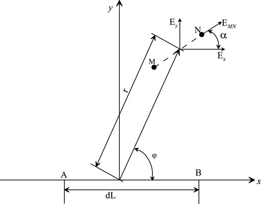
Let the electromagnetic field excited by the electric dipole source be located in the coordinate system xyz, the electric dipole source AB is parallel to the x-axis, and the angle between the receiving dipole MN and AB is (Figure 1).
The relationship between and , is obtained as follows.
According to Eq. 6, the expression for the electric field of is as follows.
The electric field expression is defined by Eq. 7.
If the number of layers N = 1, both and are equal to 1. The above equations will be transformed into the expressions for the field on a uniform earth obtained in the previous section.
Substituting Eq. 8 into Eq. 4, the accurate expression of the wide field apparent resistivity at the measurement of MN can be obtained
In Eq. 9: when , , the correct geoelectric parameters under the observation station can be obtained either by using Eq. 9 or Eq. 4; when , , the correct geoelectric parameters under the MN at the measurement end can be obtained by iterative calculation of Eq. 9. The wide field apparent resistivity parameters along the MN direction of the receiving dipole can be obtained by iteration or inverse spline difference.
2.3 Evaluation basis
When discussing the evaluation of the error caused by the azimuthal angle difference between the current source dipole AB and the receiving dipole MN, the degree of separation between the observed change value caused by and the background must be determined as a criterion, and the relative error between the apparent resistivity value of , and the apparent resistance value of , under the condition of the same frequency point is taken as a criterion in the paper.
In Eq. 10: j is the frequency number, n is the number of frequencies, is the wide field apparent resistivity value corresponding to the jth frequency at , and is the wide field apparent resistivity value corresponding to the jth frequency at .
3 Method verification
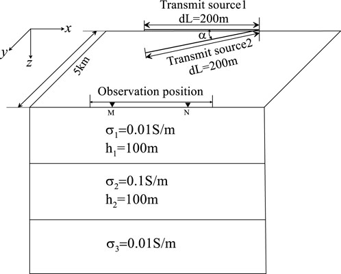
In order to verify the correctness of the calculation of the arbitrary directional wide field electromagnetic method proposed in this paper, a three-layer geoelectric model is designed: the first layer has a conductivity of and a thickness of 100 m; the second layer has a conductivity of and a thickness of 100 m; the third layer has a conductivity of ; the horizontal long wire source is laid along the x-direction with a length of 200 m and the coordinates of the center point are (0, 0, 0); the transmitting frequency range is 0.01∼10,000 Hz, the current amplitude is 1 A; the measurement line offset distance is 5 km, and the observation position (MN) laid along the x-direction (Figure 2).
Option 1: Assuming that the measurement end MN is parallel to transmit source1, i.e., , the wide field apparent resistivity is calculated by using the wide field electromagnetic method theoretical Eq. 4.
Option 2: The observation end MN is not parallel to transmit source2, and the angle between MN and dL is designed , and the wide field apparent resistivity is calculated using Eq. 4 and Eq. 9, respectively, and the relative mean square error is analyzed based on Eq. 10.
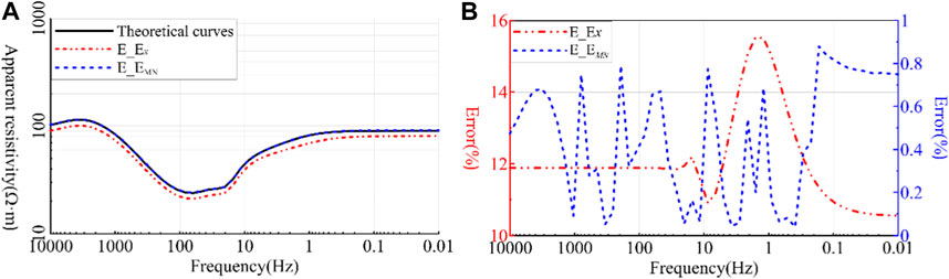
Analysis of Figure 3 shows that: ① when , the black curve in the figure relatively accurately reflects the H-type geoelectric information, in which the high-frequency resistivity value varies at 100 Ω·m and the wide field apparent resistivity value of 100∼10 Hz is 23 Ω·m; the low-frequency wide field apparent resistivity value fluctuates around 90 Ω·m.
② When , the theoretical wide field apparent resistivity Eq. 4 is still used to obtain the frequency-wide field apparent resistivity graph (see Figure 3A). (b) Comparing with the theoretical curve of curve , the two curves separate clearly, and the error curve in Figure 3B reveals that the observation error caused by the azimuthal angle difference is >10%.
③ When the azimuth angle , the wide area apparent resistivity is calculated by using the Formula 10 proposed in this paper for any orientation, and the frequency-wide field apparent resistivity curve is obtained (see Figure 3A). Comparing the theoretical curve in Figure 3A with the 3a curve line, the two curves almost overlap together, and the error curve in Figure 3B reflects that the error at each frequency point is <1%.
By designing the 3-layer theoretical model, the validity of the calculation formula of the arbitrary azimuthal wide area method is verified. The use of the arbitrary azimuthal wide field method to calculate the wide field apparent resistivity parameters can effectively reduce the influence of the observed parameters by the azimuthal angle difference and make the observed apparent resistivity parameter values closer to the theoretical calculated values. In order to further illustrate the effectiveness and correctness of the proposed method, experimental work was carried out next to a known well in Sichuan.
4 Experimental analysis
4.1 Field construction layout
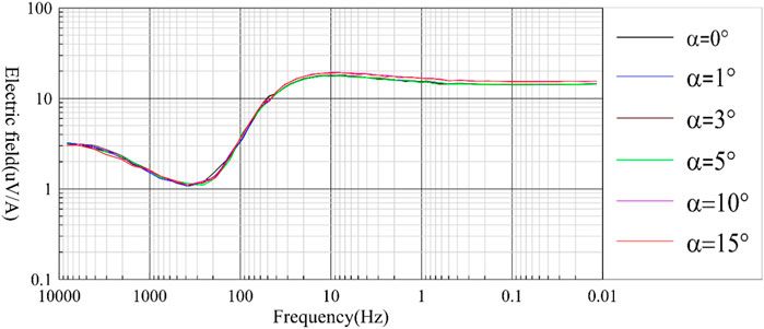
In order to analyze the effect of on the observed parameters and further verify the correctness of method in this paper. Different experimental work were carried out without obvious electromagnetic humanistic interference, in which was 0°, 1°, 3°, 5°, 10°, and 15° respectively. The field experiment scheme is shown in Figure 4: only the position of pole B is changed, while other experimental parameters remain unchanged. When , it indicates that the parallel observation position of the transmitting source AB is parallel to that of the receiving end MN, and there is no azimuth Angle difference.
This field using pseudo-random 7-frequency wave signal, that is, a simultaneous transmission and reception from the underground 7 frequency signals. The parameters of this experiment: current transmitting source AB = 1 km, receiving end MN = 100 m, transmitting current I = 80 A, keeping the intensity of transmitting current constant, transmitting frequency range 8,192∼0.01 Hz, total 54 frequency points.
To eliminate the effect of current, the observed potential difference data were normalized by current and the “frequency-electric field” curves were plotted along the MN direction for different conditions (Figure 5). From the analysis of Figure 5, the difference of electric field caused by different is small, and it is difficult to discern the influence of on the observation results intuitively. In the later analysis, the influence of on the observation results is analyzed from the apparent resistivity parameter, and the validity and correctness of the calculation formula proposed in this paper are verified.
4.2 Analysis of experimental results
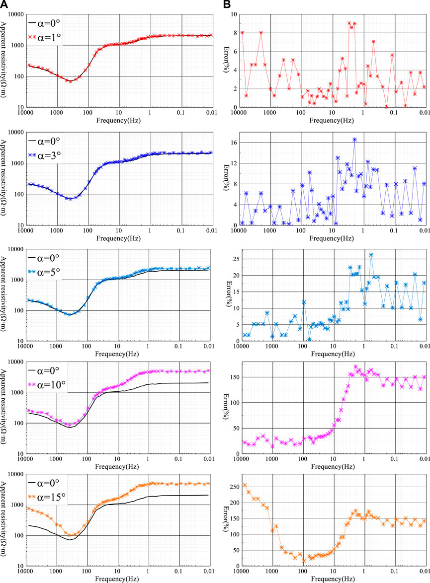
Figure 5 shows the “frequency-apparent resistivity” graph and “frequency-relative error” graph for different azimuthal differences without considering the effect of azimuthal difference , but directly calculated by inverse spline numerically from Eq. 4. The analysis of the “frequency-apparent resistivity” graph and the relative error graph in Figure 6 is shown as follows.
(1) When , the corresponding “frequency-apparent resistivity” curve is the same as the “frequency-apparent resistivity” curve with , and there is no obvious separation, and the relative error of the corresponding apparent resistivity is ≤5%, while the relative error of the apparent resistivity of individual frequency points is >5%. The relative error of the apparent resistivity at individual frequency points is >5%. It means that the azimuthal difference between the current source AB and the receiver MN has a small effect on the wide field apparent resistivity.
(2) When , the “frequency-apparent resistivity” curve of Figure 6 and the “frequency-apparent resistivity” curve of have no obvious separation in the frequency band (8,192∼10 Hz), and the relative error of each frequency point is ≤10%; in the middle and low There is a weak separation in the frequency band (10∼0.011 Hz), and the relative error at each frequency point varies from 10% to 25%.
(3) When , the “frequency-apparent resistivity” curve of Figure 6 and the “frequency-apparent resistivity” curve of do not show significant separation in the frequency band (8,192∼10 Hz), and the relative error of each frequency point is ≤10%; in the middle and low frequency band (10∼0.011 Hz), the separation is more obvious, and the relative error of each frequency point is ≤15%. (10∼0.011 Hz), with relative error ≤15% at each frequency point.
(4) When , the “frequency-apparent resistivity” curves of Figure 6 and both show a clear separation, and even the shape of the curves changes in the low and middle frequency bands (30∼0.01 Hz). In the high-mid frequency band (8,192∼10 Hz), the relative error of apparent resistivity at each frequency point varies from 20% to 40%; in the low-mid frequency band (10∼0.01 Hz), the relative error ranges from 100% to 170%. It indicates that the azimuthal difference between the current source AB and the MN at the receiver has a large effect on the wide field apparent resistivity of the full frequency band, even causing distortion of the apparent resistivity parameters.
(5) When , the “frequency-apparent resistivity” curve of Figure 7 and the “frequency-apparent resistivity” curve of both show significant separation, and the shape of the curves in the high-middle frequency band (8,192∼10 Hz) and the low-middle frequency band (30∼0.01 Hz The curves in the high-mid frequency band (8,192∼10 Hz) and the low-mid frequency band (30∼0.01 Hz) have changed or even become distorted. The relative error range of the apparent resistivity at each frequency point in the high-mid frequency band (8,192∼10 Hz) varies from 40% to 255%; the relative error range in the mid-low frequency band (10∼0.01 Hz) is greater than 100%. This indicates that the azimuthal difference between the current source AB and the receiver MN has a large effect on the wide field apparent resistivity in the full frequency band, causing distortion of the apparent resistivity parameters.
From the above analysis, it can be concluded that: in the range of , the azimuthal difference has a small effect on the apparent resistivity parameters; when , the azimuthal difference aa mainly affects the apparent resistivity parameters in the middle and low frequency bands; when , the azimuthal difference aa has a large effect on the apparent resistivity parameters in the whole frequency band, and the more serious the distortion of the high-middle frequency data, the more obvious the false anomaly caused, and even causes the interpretation of the parameter distortion. If the relative error of the apparent resistivity value ≤10% is considered reasonable, it must be ensured that , but the field construction conditions are restricted by the terrain, and it is often difficult to achieve the azimuthal difference between the current source AB and the receiver MN, so the angle correction must be made to the observed data to eliminate the influence brought by and improve the interpretation accuracy of the apparent resistivity parameters.
4.3 Analysis of experimental results
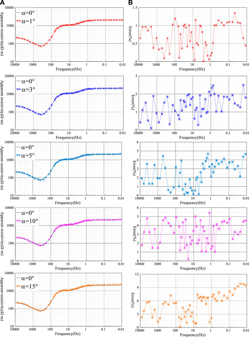
Figure 7 shows the “frequency-apparent resistivity” curve and the relative error curve calculated and plotted according to the arbitrary orientation of Eq. 9. The analysis of the “frequency-apparent resistivity” curve and the relative error graph in Figure 7 is shown as follows.
(1) When , the “frequency-apparent resistivity” curve of Figure 7 and the “frequency-apparent resistivity” curve of do not show significant separation and approximately coincide, and the relative error of the apparent resistivity at each frequency point is ≤1%, which is reduced from 8% to 1% compared with the calculation of Figure 6.
(2) When , the “frequency-apparent resistivity” curve of Figure 7 and the “frequency-apparent resistivity” curve of do not show significant separation and almost coincide, and the relative error of the apparent resistivity at each frequency point corresponds to a range of (−2% ∼ 2%), which is reduced from 15% to 2% compared with the calculation of Figure 6 .
(3) When , the “frequency-apparent resistivity” curve of Figure 7 and the “frequency-apparent resistivity” curve of do not show any obvious separation, and the shape of the curve changes similarly, and the relative error of the corresponding apparent resistivity at each frequency point changes in the range of (−4% ∼ 4%), compared with the relative error of Figure 6 calculation method from 25% to 4%.
(4) When , the “frequency-apparent resistivity” curve of Figure 7 is not significantly separated from the “frequency-apparent resistivity” curve with . The curve shape changes similarly, and the relative error of the apparent resistivity at each frequency point is (−4% ∼ 5%), which is reduced from 150% to 5% compared with the relative error of Figure 6 calculation.
(5) When , there is no obvious separation between the “frequency-apparent resistivity” curve in Figure 7 and the “frequency-apparent resistivity” curve with . The shape of the curve changes similarly, and the relative error of the apparent resistivity at each frequency point varies in the range of (−7% ∼ 10%), which is reduced from 300% to 10% compared with the relative error of the calculation in Figure 6.
The analysis results of Figures 6, 7 show that: firstly, the maximum relative error of the wide area apparent resistivity obtained by the arbitrary azimuthal wide area electromagnetic method is reduced from 25% to 4% when , which makes the apparent resistivity parameter closer to the real underground geoelectric information; secondly, the relative error of the wide area apparent resistivity obtained by the arbitrary azimuthal wide area electromagnetic method is reduced from 270% to less than 10% when and . Thirdly, if the azimuth angle difference is larger, the effect of using method of arbitrary azimuth wide field electromagnetic method on eliminating is more obvious, which reflects the real resistivity value of the subsurface and improves the accuracy of the wide field apparent resistivity effectively.
4.4 Analysis of inversion effect
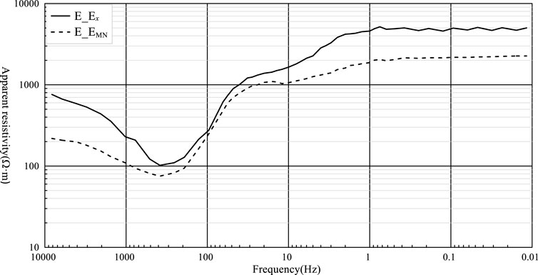
In this section, we take as an example, and perform single-point inversions of and apparent resistivity respectively, and further analyze the effect of azimuthal difference on the interpretation parameters by combining the electric logging data of Ning 227 borehole. One-dimensional continuum imaging was performed on the processed data, and the relevant parameters of inversion were as follows: inversion depth was 4.5 km; The number of iterations in the inversion process was 20; The horizontal and depth resolution were 1; The regularization parameter was 5; The fitting error was 0.02. Figure 8 shows the bathymetric curves of “frequency-apparent resistivity” obtained from different calculation methods of and , and the single-point inversion curves are shown in Figure 9.
(1) From Figure 8 and “frequency-apparent resistivity” curve analysis, it can be seen that when the azimuth angle difference is 15°, the corresponding “frequency-apparent resistivity” sounding curves of different calculation methods of the same measurement point are different, and the two curves are completely separated, and the curve change pattern is also different, which means that the azimuth angle difference α has a greater influence on the apparent resistivity parameter.
(2) From the comparative analysis of the single-point inversion curve and the drilling electric logging curve in Figure 9, it can be obtained that: Firstly, above elevation 0 km, both and have less variability and are in basic agreement with the trend of the logging resistivity curve, and the electrical stratification of the single-point inversion curve is obvious. Secondly, the variation patterns of depth-resistivity curves of and after single-point inversion in the middle and deep parts (0∼−3 km) differ greatly, in which the variation trends of mode curves are generally more consistent with the variation trends of electric logging curves and the resistivity stratification is also obvious, while the variation trends of curves are more consistent with the variation trends of electric logging curves and the electrical stratification is weaker. Thirdly, from the analysis of the inversion iteration error curve in Figure 9, it can be seen that the number of iterations of apparent resistivity inversion is 6, and the error decreases from 33% to about 2%, and the error almost no longer changes with the increase of the number of iterations; on the contrary, the number of iterations of apparent resistivity inversion is 10, and the error decreases from 34% to 3.8%, and the inversion fitting error no longer changes with the increase of the number of iterations. Therefore, the inversion of the apparent resistivity parameter can achieve a more satisfactory fitting error with fewer iterations.
(3) The use of arbitrary azimuthal wide area electromagnetic method observation method for field observation data can effectively reduce the observation error caused by azimuthal angle difference, improve the validity and accuracy of the interpretation parameters, and also greatly reduce the construction requirements of wide area electromagnetic method field current source AB parallel receiving dipole MN, improve the field production efficiency and save economic costs, which has important research significance and practical production significance.
5 Conclusion
In order to eliminate the influence of azimuthal angle difference α to the observation parameters and improve the validity and accuracy of the interpretation parameters, we proposed an arbitrary observation orientation wide field electromag-netic method in this paper, i.e., calculating the wide field apparent resistivity parameters along the MN direction of any measurement end. Based on the results of theoretical model orthorectification and field measurement data, the following conclusions are obtained:
(1) The three-layer geoelectric model and two observation schemes are designed, and by comparing with the theoretical method E_Ex, the method calculation method is adopted, which effectively eliminates the influence of azimuthal angle difference α to the apparent resistivity parameters and verifies the effectiveness and correctness of the arbitrary azimuthal wide field electromagnetic method E_EMN.
(2) The experimental work of different azimuth angle difference α was carried out beside the well, and the calculation parameters of wide field electromagnetic method E_Ex and arbitrary azimuth wide field electromagnetic method E_EMN were compared and analyzed. The results show that: Firstly, when α ≤ 5°, at the same frequency of the same measuring station, the maximum relative error of the wide field apparent resistivity value using any azimuth E_EMN method decreases from 30% to 4% compared with the E_Ex method, which effectively improves the accuracy of the apparent resistivity value and makes the qualitative analysis more accurate; Secondly, when α = 10° and 15°, the relative error of the whole band apparent resistivity value of E_Ex calculation method is not less than 50%, the maximum is 300%, and the apparent resistivity parameter is seriously distorted. Using any azimuth E_EMN calculation method, the maximum relative error of the all-band apparent resistivity decreases from 300% to less than 10%; Thirdly, the single station inversion results of different methods show that the arbitrary azimuth E_EMN calculation method can achieve a relatively ideal fitting error with fewer iterations, and the interpretation parameters are closer to the actual formation electrical information, improving the accuracy of resistivity parameter. Arbitrary azimuth wide field electromagnetic method E_EMN can effectively reduce the observation error caused by azimuth angle difference α, and can directly and truly reflect the objective change of geoelectric section with depth, which makes the electrical analysis more accurate, and further verifies the validity and reliability of the calculation method in this paper.
(3) The wide field apparent resistivity parameters obtained by the arbitrary orientation method can effectively eliminate the observation error caused by α between the current source dipole AB and the receiving dipole MN, which greatly improves the accuracy of the wide field apparent resistivity parameters, and also better expands the applicability and flexibility of the current source wide field electromagnetic method in complex terrain areas, with important theoretical research and practical production significance.
Data availability statement
The original contributions presented in the study are included in the article/supplementary material, further inquiries can be directed to the corresponding author.
Author contributions
Author ZT Mainly to assist in field experiments. All authors listed have made a substantial, direct, and intellectual contribution to the work and approved it for publication.
Conflict of interest
Author ZT was employed by Sichuan Zhongcheng Coal Field Geophysical Engineering, Research Institute Co., Ltd.
The remaining authors declare that the research was conducted in the absence of any commercial or financial relationships that could be construed as a potential conflict of interest.
Publisher’s note
All claims expressed in this article are solely those of the authors and do not necessarily represent those of their affiliated organizations, or those of the publisher, the editors and the reviewers. Any product that may be evaluated in this article, or claim that may be made by its manufacturer, is not guaranteed or endorsed by the publisher.
References
Cagniard, L. (1953). Basic theory of the magnetotelluric method of geophysical prospecting. Geophysics 18 (3), 605–635. doi:10.1190/1.1437915
CrossRef Full Text | Google Scholar
Cao, C. Q. (1978). The apparent resistivity for layered Earth. Chin. J. Geophys. 21 (3), 248–261.
Google Scholar
Chen, H., and Li, D. Q. (2014a). A new electromagnetic field division method for horizontal electric dipole. J. Central South Univ. Sci. Technol. 45 (7), 2250–2258.
Google Scholar
Chen, M, S. (2014b). The electromagnetic field distribution and observation parameters. Coal Geol. Explor. 42 (5), 81–86. doi:10.3969/j.issn.1001-1986.2014.05.016
CrossRef Full Text | Google Scholar
Dai, S. K., Zeng, L., Zhou, Y. M., Li, K., Chen, Q. R., and Ling, J. X. (2020). Research on direct integration algorithm of electromagnetic field in homogeneous layered media for a wide range of frequencies and transceiver distances. Oil Geophys. Prospect. 55 (6), 1364–1372.
Google Scholar
Fang, W. Z., Li, X., Li, Y. G., and Feng, B. (1992). The whole-zone definition of apparent resistivity used in the frequency domain electromagnetic methods. J. Xi’an Coll. Geol. 14 (4), 81–86.
Google Scholar
Goldstein, M. A. (1971). Magnetotelluric experiments employing an artificial dipole source. Toronto, Canada: University of Toronto.
Google Scholar
He, J. S. (2019). Theory and technology of wide field electromagnetic method. Chin. J. Nonferrous Metals 29 (9), 1809–1816.
Google Scholar
He, J. S. (2020). New research progress in theory and application of wide field electromagnetic method. Geophys. Geochem. Explor. 44 (5), 985–990.
Google Scholar
He, J. S. (2010a). Wide field electromagnetic sounding methods. J. Central South Univ. Sci. Technol. 41 (3), 1065–1072. doi:10.1190/segam2015-5835894.1
CrossRef Full Text | Google Scholar
He, J. S. (2010b). Wide field electromagnetic sounding methods and pseudo-random signal coding electrical method. Beijing, China: Higher Education Press.
Google Scholar
Huang, H. P., and Piao, H. R. (1992). Full-wave apparent resistivity from vertical magnetic dipole frequency sounding on a layered Earth. Chin. J. Geophys. 35 (5), 389–395. in Chinese.
Google Scholar
Li, D. Q. (2017). Measurement range of E_Ex and E_Eφwide field elegytromagnetic methods. Oil Geophys. Prospect. 52 (6), 1315–1323.
Google Scholar
Li, G., Wu, S. L., Cai, H. Z., He, Z. S., et al. (2023). A new deep temporal convolutional network combined with dictionary learning for strong cultural noise elimination of controlled-source electromagnetic data. Geophysics 88 (4). doi:10.1190/geo2022-0317.1
CrossRef Full Text | Google Scholar
Liu, J. X., Tong, T. G., Liu, C. M., et al. (2013). Recognition of electromagnetic field asymptotic properties and improved definition of wide field apparent resistivity on E−Eφ array. Chin. J. Nonferrous Metals 23 (9), 2359–2364.
Google Scholar
Liu, J. X., Liu, R., Guo, R. W., Tong, X. Z., and Xie, W. (2022). Research progress of electromagnetic method in nonferrous metal mineral exploration. Chin. J. Nonferrous Met. 33 (1), 261–284.
Google Scholar
Liu, J. X., Zhao, R., and Guo, Z. W. (2019). Research progress of electromagnetic methods in the exploration of metal deposits. Prog. Geogr. (in Chinese) 34 (1), 0151–0160. doi:10.6038/pg2019CC0222
CrossRef Full Text | Google Scholar
Mao, X. J., and Bao, G. S. (1996). A direct algorithm for full-wave apparent resistivity from horizontal electric dipole frequency sounding. J. Cent. South Univ. Technol. 27 (3), 254–257.
Google Scholar
Spies, B. R., and Eggers, D. E. (1986). The use and misuse of apparent resistivity in electromagnetic methods. Geophysics 51 (7), 1462–1471. doi:10.1190/1.1442194
CrossRef Full Text | Google Scholar
Tang, J. T., and He, J. S. (1994). A new method to define the full-zone resistivity in horizontal electric dipole frequency sounding on a layerd Earth. Chin. J. Geophys. 3 (4), 543–552.
Google Scholar
Tang, J. T., and He, J. S. (2005). Controlled source audio-frequency magnetotelluric method and its application. Changsha, China: Central South University Press.
Google Scholar
Tang, J. T., and He, J. S. (1993). Effective resistivity defined by the electromagnetic fields induced by horizontal electric dipole. J. Cent. South Univ. Technol. 24 (2), 137–142.
Google Scholar
Tikhonov, A., N. (1950). On determining electrical characteristics of the deep layers of the Earth's crust. Dokl. Akad. Nauk. SSSR 73, 295–297.
Google Scholar
Wang, H. Y., Guo, W. B., and Liu, Y. A. (2021). “Research and application of ground-well frequency domain electromagnetic method,” in Proceedings of the First National Conference on Mineral Exploration, Barcelona, Spain, September 2016, 55–58. Chinese Geophysical Society (Chinese Geophysical Society: Chinese Geophysical Society.
Google Scholar
Wang, S. G., Xiong, B., and Dai, S. K. (2013). Analysis of resolution ability to E-Ex arrangement wide field electromagnetic method using 1-D modeling and inversion. J. Central South Univ. Sci. Technol. 44 (9), 3766–3774.
Google Scholar
Wang, S. G., and Xiong, B. (2012). Numerical calculation methods of wide field apparent resistivity. Comput. Tech. geopaysical Geochem. Explor. 34 (4), 0380–0383. doi:10.1002/cjg2.419
CrossRef Full Text | Google Scholar
Yin, C. C. (1991a). Forward calculation and application of frequency domain sounding at any azimuth. Comput. Tech. Geophys. Geochem. Explor. 13 (2), 129–138.
Google Scholar
Yin, C. C., and Piao, H. R. (1991b). A study of the definition of apparent resistivity in electromagnetic sounding. Geophys. Geochem. Explor. 15 (4), 290–299.
Google Scholar
Yu, Y. C. (2010). Wide field electromagnetic method of one-dimensional positive inversion. Changsha, Hunan: Central South University.
Google Scholar
Yuan, B., Li, D. Q., and Hu, Y. F. (2020). New correction method for controlled-source electromagnetics source effects. Trans. Nonferrous Metals Soc. China 30 (12), 3356–3366. doi:10.1016/S1003-6326(20)65467-X
CrossRef Full Text | Google Scholar
Zonge, K. L., and Hughes, L. J. (1991). Controlled source audio-frequency magnetotellurics. Electromagn. Methods Appl. Geophys. 2. Application, Parts A and B. doi:10.1190/1.9781560802686.ch9
CrossRef Full Text | Google Scholar
 Hongjun Tian
 Jianke Qiang1,2*