Accuracy assessment of various supervised machine learning algorithms in litho-facies classification from seismic data in the Penobscot field, Scotian Basin

Litho-facies classification is an essential task in characterizing the complex reservoirs in petroleum exploration and subsequent field development. The lithofacies classification at borehole locations is detailed but lacks in providing larger coverage areas. The acquired 3D seismic data provides global coverage for studying the reservoir facies heterogeneities in the study area. This study applies six supervised machine learning techniques (Random Forest, Support Vector Machine, Artificial Neural Network, Adaptive Boosting, Xtreme Gradient Boosting, and Multilayer Perceptron) to 3D post-stack seismic data to accurately estimate different litho-facies in inter-well regions and compares their performance. Initially, the efficacy of the said models was critically examined via the confusion matrix (accuracy and misclass) and evaluation matrix (precision, recall, F1-score) on the test data. It was found that all the machine learning models performed best in classifying the shale facies (87%–94%) followed by the sand (65%–79%) and carbonate facies (60%–78%) in the Penobscot field, Scotian Basin. On an overall accuracy scale, we found the multilayer perceptron method the best-performing tool, whereas the adaptive boosting method was the least-performing tool in classifying all three litho-facies in the current analysis. While other methods also performed moderately good for the classification of all three litho-facies. The predicted litho-facies using seismic attributes matched well with the log data interpreted facies on the borehole locations. It indicates that the facies estimated in inter-well regions are accurate and reliable. Furthermore, we validated the estimated results with the other seismic attributes to ascertain the accuracy and reliability of the predicted litho-facies between the borehole locations. This study recommends machine learning applications for litho-facies classification to reduce the risk associated with reservoir characterization.

1 Introduction

Accurate identification of the lithological types is essential in discriminating the reservoir facies (sand and carbonate) from the background (shale facies). It can also be done through advanced high-resolution image logs as well as laboratory investigations of drilled core samples. However, such high-resolution field measurement data is commonly limited (available only at well positions) and expensive (Kumar et al., 2022; Srivardhan, 2022). On the other hand, seismic data interpretation provides global coverage but has lower vertical resolution and non-unique solutions. In seismic data interpretation, geoscientists always strive to determine the connection between geophysical datasets and reservoir properties in order to forecast lithological distributions. It has been found that obtaining a reliable lithological model, particularly seismic data, is one of the most challenging tasks in reservoir studies. In recent years, machine learning (ML) techniques have emerged as an effective tool in dealing with geophysical data (MacLeod, 2019; Dramsch, 2020). As a result, integrating ML algorithms with the inputs of existing petrophysical and geophysical data enables geoscientists to categorize the different lithologies precisely. Several studies have successfully identified litho-facies on geophysical logs using statistical approaches, and supervised and unsupervised ML algorithms (Wang and Carr, 2012; Schmitt et al., 2013; Bhattacharya et al., 2016; Bressan et al., 2020; Xu et al., 2021), and reservoir characterization in petroleum exploration (Keynejad et al., 2019; Liu et al., 2021). On the other hand, only a few research works have been done to determine the various litho-facies and reservoir properties using seismic data (Zhang and Zhan, 2017; Chevitarese et al., 2018; Babu et al., 2022).

The supervised ML technique structure primarily consists of input, hidden, and output layers. Among all, Random Forest (RF), Artificial Neural Network (ANN), Adaptive Boosting (ADB), Extreme Gradient Boosting (XGB), Support Vector Machine (SVM), and Multilayer Perceptron (MLP), etc., are a few supervised regression and classification algorithms. These methods use forward and backward propagation to reduce error between the predicted and original values. In classification problems, the classifier’s accuracy between the original and predicted values depends on the confusion matrix (accuracy and misclass) and evaluation matrix (precession, recall, and F1-score) (Xu et al., 2021). The seismic-derived attributes listed in Table 2 are input features, whereas the litho-facies interpreted at wells (log-scale) is the target feature during the model training (Babu et al., 2022). Initially, all the input data were randomized and standardized to avoid bias. ML algorithms have been trained to classify the different litho-facies on 75% of total data samples, and the left out 25% of data samples were used for validation purposes. We classified these facies into three categories which are coded as shale facies (1), sand facies (2) and carbonate facies (3). We performed six popular classification algorithms in the current work to predict the litho-facies from the Penobscot field, Scotian Basin.

The primary objective of the current research work is to evaluate the performance of the applied ML models (RF, ANN, ADB, XGB, SVM and MLP) in litho-facies (shale, sand, and carbonate) prediction away from borehole locations using seismic data. Secondly, to delineate and characterize the reservoir facies from Mississauga and Abenaki Formation based on interpreted litho-facies. Moreover, these predicted litho-facies require further validation using other seismic attributes to ascertain the models’ predictions in inter-well regions. The present study explained the practical approach in litho-facies discrimination and provides a reliable lithological model for hydrocarbon exploration from Mississauga and Abenaki Formation using seismic data.

2 Geological settings

The Penobscot field is located on the Scotian Shelf (Figure 1). It has a large-scale carbonate bank that originated during the Jurassic era as the Sable Delta prograde into the basin (Eliuk and Crevello, 1985). It is approximately 1,200 km south-westward from the Yarmouth Arch to the north-eastward Avalon Uplift on Newfoundland’s Grand Banks and contains numerous structural and stratigraphic features (Jansa et al., 1989; Weissenberger et al., 2006). Scotian Basin development started after the breakup and rifting of the North American continent from the African continent at the end of Triassic period. The study area contains numerous complex structural and stratigraphic features in the subsurface. Several minors but two NW-SE and E-W trending major faults have been identified in the study area (Campbell et al., 2015; Bhatnagar et al., 2017; Maurya, 2019). Early Jurassic (Mid-Sinemurian) tectonic activity in the central rift basin led to complex faulting, erosion of Late Triassic and Early Jurassic sediments and older deposits. Generalized stratigraphic chart for Scotian Basin is shown in Figure 2. The region’s sediment distribution has been greatly influenced by the network of platforms and subbasins. An initial transition (Anisian to Toarcian) from terrestrial rift sediments to shallow marine carbonates and clastic, followed by an initial post-rift carbonate-dominated phase (Aalenian-Tithonian), characterizes early deposition in the area (NSDE, 2011). The second post-rift sequence (Berriasian-Turonian) consists of a thick, rapidly deposited deltaic wedge (Mississauga Formation) and a series of thinner, backstepping deltaic lobes (Logan Canyon Formation). Overall, a vast history of passive-margin deposition dominates the stratigraphic framework in the region, which is episodic. A detailed workflow adopted in this work is shown in Figure 3.

FIGURE 1

FIGURE 1. Location map of the study area in the Scotian Basin, Canada Offshore.

FIGURE 2

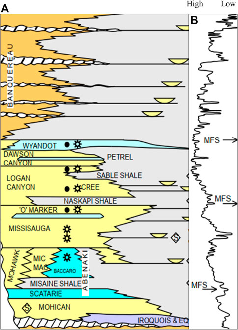
FIGURE 2. (A) Stratigraphy chart of the Scotian Basin (after MacLean and Wade, 1993; Wade et al., 1995; NSDE, 2011), and (B) Eustatic curve indicating the sea-level changes during different geological stages (Haq et al., 1987).

FIGURE 3

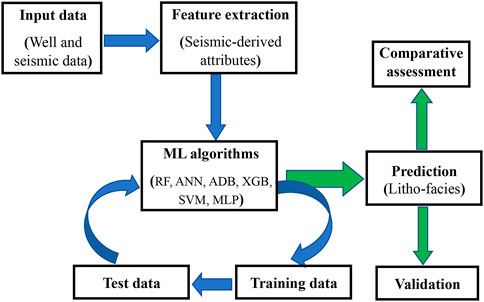
FIGURE 3. Flow chart for the adopted methodology in litho-facies prediction in the present study.

3 Data

The study area have two drilled wells (L-30 and B-41). These wells consist recorded conventional logs viz., gamma-ray (GR), compressional wave (DT), density (RHOB), spontaneous potential (SP) and density-porosity (DPHI) and neutron-porosity (NPHI) logs (Kidston et al., 2005). We interpreted the three different litho-facies (shale, sand, and carbonate) based on electro-log interpretation (Figures 4A, B). Manual litho-facies interpretation is tedious but has the least chance of error. The obtained result was validated with available core data from well L-30 at 2167 ms (Jansa et al., 1989), corresponding to the Abenaki Formation. The core data suggests the presence of Thrombolites, Stromatolites, Mudstone, and Wackestone, a typical signature of carbonate facies. The seismic and log data and formation tops and horizons obtained from the publicly available Canada-Nova Scotia offshore petroleum board directory have been downloaded from the OpendTect data portal. 3D seismic data acquired during the year 1992 over the Penobscot field in the Scotian Shelf, Nova Scotia, Canada, has been used in this study (Figure 5A). The seismic data were recorded over a 90.27 km² area in a bin size of 12.5 m (inline) × 25 m (crossline). The data was recorded up to 6s with a sampling interval of 4 ms with good frequency bandwidth (6–50 Hz) up to 3 s. The seismic signal below 3s (5 km) is poor (Maurya, 2019; Ray et al., 2022). We performed well-to-seismic-tie for both wells to establish a time-depth relationship in the study area (Figure 5B). Table 1 summarises the specifics of the seismic and well-log data.

FIGURE 4

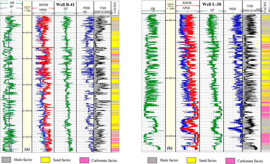
FIGURE 4. Well panel showing the different logs and interpreted litho-facies from wells (A) B-41 and (B) L-30.

FIGURE 5

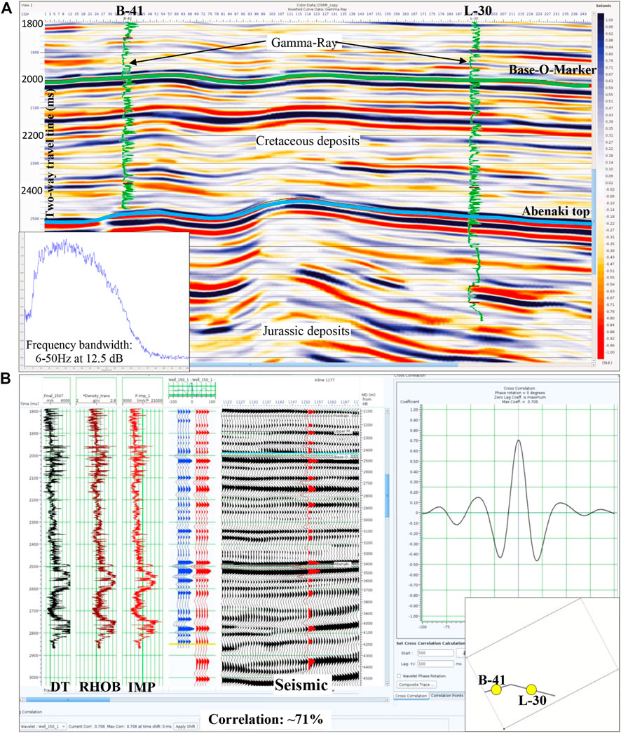
FIGURE 5. (A) An arbitrary line section extracted from the seismic data passing through both wells in the study area (basemap in inset). Frequency bandwidth (6–50 Hz) found for this seismic data, and (B) well-to-seismic tie at L-30.

TABLE 1

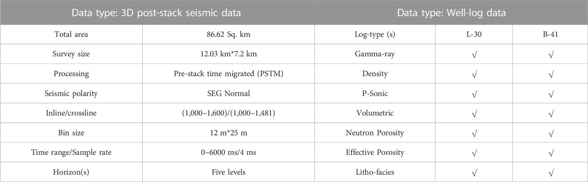
TABLE 1. 3D seismic and well log data available in the study area.

4 Different ML algorithms

4.1 Random forest (RF)

A supervised ensemble learning method based on the random subspace methodology, the RF algorithm was first proposed by Ho (1995). Later, based on the bagging strategy, Breiman (1996) updated this method. With this approach, sample subsets are taken from the main database, and decision trees are generated for each sample space to classify patterns. The majority of the forest’s trees’ output is chosen via a vote process. The bagging approach of RF enhances overall accuracy and reduces overfitting problems since it uses the mean of predictions generated from numerous choices’ trees (Breiman, 2001).

4.2 Artificial neural network (ANN)

Finding the ideal collection of weight parameter values is the goal of the neural network procedure. Use of the backpropagation technique is common in layered feed-forward ANNs. This algorithm adjusts weights to decrease system error within network.

It may be organized into four basic steps: a) Set random values as the connection weights’ initial values. b) Calculate the ANN’s output by forward propagating each input pattern through the network:

$E_k={\displaystyle \sum _{i=1}^n}{\left({\mathrm{t}}_i-a_i\right)}^2(1)$

(c) Eq. 1 used to calculate the Mean Square Error ($E_k$) between the desired output (${\mathrm{t}}_i$) and what was actually produced ($a_i$) by the ANN.

$W_{t+1}=W_t+-\eta \frac{d{E}_k}{dw}(2)$

(d) Eq. 2, where $W_t$ is weight, $\frac{d{E}_k}{dw}$ is the gradient and $\eta$ is the learning rate, should be used to adjust the connection weights. This procedure is continued until the desired minimum error is achieved.

4.3 Adaptive boosting (ADB)

Freund and Schapire (1997) introduced the AdaBoost or Adaptive Boosting method after first discussing it in 1995. Through the multiplicative-weight update technique, weaker ML “algorithms” performance can be enhanced without any prior knowledge. Taking into account that the output of a weak learning algorithm f′ is represented as OP′1, OP′2 ….OP′m and that the goal of the weak learner is to fit a function f′ between TR and OP by least square error, which is (OP- f′ (x′))², where x′ € TR. The error function for adaptive boosting is $e^{-OP{f}^{\prime }\left({\mathrm{x}}^i\right)}$, which only considers the final result’s sign. The final error is the multiplicative addition of all of the previous errors, that is $e^{-{\displaystyle \sum }_{i}O{P}_i{f}^{\prime }\left({\mathrm{x}}^{\prime }\right)}$. The method updates the weights at each stage and segment of the iteration to identify segments that tend to increase the error and alter the weights in order to reduce the error.

4.4 Extreme gradient boosting (XGB)

According to Chen and Guestrin (2016), the supervised machine learning algorithm XGB uses gradient boosting to handle massive data series. This ensemble technique continuously builds new predictors (decision trees) until the error introduced by its early predictors is eliminated. XGB uses residual values to create a series of weak learners before producing a strong one at the end. For preventing overfitting difficulties and punishing the problem’s complexity (Sun et al., 2020), a regularisation term is added to the loss function, which is provided by,

$l\left(\phi \right)={\displaystyle \sum }_{i}L\left(y_i-\widehat{y_i}\right)+{\displaystyle \sum _k^n}\mathrm{\Omega }f\left(k\right)(3)$

Where L, which stands for the loss function, expresses the discrepancy between the prediction ($\widehat{y_i}$) and of the target y_i. The second term ($\mathrm{\Omega }\left(f_k\right)$) penalizes the model’s complexity. The regularisation term prevents overfitting and reduces the problem’s complexity. These terms for regularisation are provided as follows:

$\mathrm{\Omega }f\left(k\right)=\gamma T+\frac{1}{2}\lambda {‖w‖}^2(4)$

The regularisation parameters in this case, denoting the leaf number and weight. Whereas w and T, respectively, represent the leaf node’s value and the number of leaves in the tree.

4.5 Support vector machine (SVM)

For classification and regression issues, the supervised machine learning method SVM is frequently utilized (Vapnik, 1995). A hyperplane is built in the SVM method to divide the datasets into several classes. The support vectors are the data points that are closer to hyperplane on either side, and the street is separation between support vectors. A hyperplane with a wide margin or street is seen to be a decent classification, while one with a narrow margin is unsatisfactory and requires further parameter adjustment.

Consider a situation where the data are linearly separable: y = sign($w^{T}x+b$).

D = (x₁, y₁), (x₂, y₂), (x_n, y_n) for training data with n points, where y_iℰ = (1, 1).

Given by is the Euclidean distance from x_i to the hyperplane:

$r=\frac{\left|w^{T}x+b\right|}{\lceil w˥}(5)$

SVM seeks to maximize ${‖w‖}^2$ and offers the optimal optimization for the issue as:

$\left(w^{*},b^{*}\right)=\underset{w,\mathrm{b},{\xi }_i}{\mathrm{a}\mathrm{g}\mathrm{r}\mathrm{m}\mathrm{i}\mathrm{n}}\frac{{‖w‖}^2}{2}+C{\displaystyle \sum _{i=1}^m}{\xi }_i(6)$

Where w and b stand for the hyperplane’s normal vector and intercept, respectively. The penalty and slack parameters, represented by C and ${\xi }_i$ control the trade-off between accurate data classification and smooth decision boundaries. SVM uses kernel trickery, which is non-linearly separable data points from the existing dimension to a higher, linearly separable dimension, for a model where the separation of the data points is non-linear. The classification problem’s radial basis function kernel is defined as follows:

$K\left(x_i,x_j\right)={\exp }^{\left(-\gamma {‖x_i-x_j‖}^2\right)}(7)$

Where, $\gamma =\frac{1}{2{\sigma }^2}$ determines the degree of bending required for the decision boundary.

4.6 Multilayer perceptron (MLP)

A perceptron is a popular neural network approach for binary issue solving through monotonically rising activation functions (Dixit and Mandal, 2020). A basic perceptron model is a mathematical representation of how the human brain works. It takes input data from the input layer, weights it, adds it all up, sends it to the activation function, and then outputs it through the output layer. Assume that the input vectors are x₁, x₂, . . . . . . . x_n and the weights are w₁, w₂, . . . . . . . w_n. A perceptron’s output is represented by,

$y={\displaystyle \sum _{i=1}^n}{w}_i{x}_i+bias(8)$

which is also written as,

$y=w^{t}x+bias(9)$

The performance of the network is determined by the number of hidden layers. The neural network performs poorly when there are few layers in between, and when there are many layers, the neural network memorizes the training data and fails on the unknown datasets (McCormack, 1991). In order to create a better MLP model, the number of neurons in the hidden layers between the input and output layers should be modified together through appropriately updated weights (Van der Baan and Jutten, 2000).

5 Results

5.1 Evaluation of ML methods in litho-facies prediction

In this research work, 6 ML classification models (RF, ANN, ADB, XGB, SVM, and MLP) were trained to predict the clastic (shale and sand) and non-clastic (carbonate) litho-facies from seismic data in Penobscot field, Scotian Basin. Initially, these models were trained on 75% of the datasets (termed training data). Further, the trained models were validated on left out 25% of the datasets (termed as test data). The seismic-derived attributes utilized in litho-facies prediction are listed in Table 2. We calculated the evaluation matrix, such as Precision, Recall, and F1-score of each predictive method for each litho-type, to assess the model performance on the test data (Figure 6; Table 3). Additionally, a normalized confusion matrix (accuracy and misclass) was computed to evaluate each applied ML technique in this study (Figures 7, 8; Table 4). The maximum attainable value for the above parameters is 1.

TABLE 2

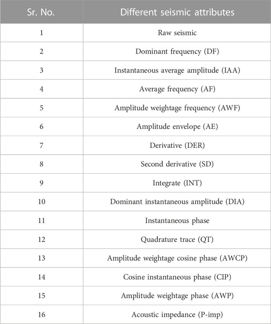
TABLE 2. Input 3D seismic attributes used in litho-facies prediction.

FIGURE 6

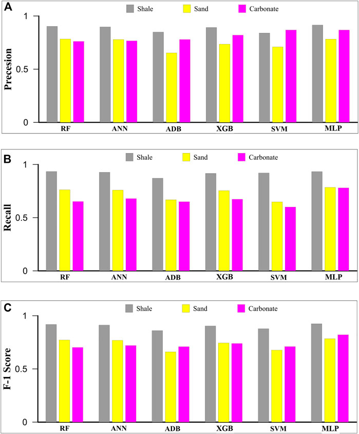
FIGURE 6. Outputs of each predictive model’s evaluation metrics (A) precision, (B) recall, and (C) F1 score, computed for each litho-facies.

TABLE 3

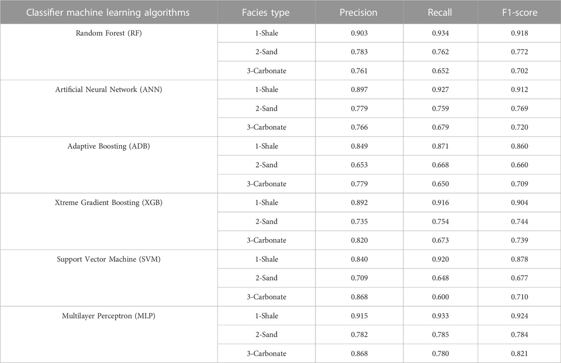
TABLE 3. Statistics, i.e., Precision, Recall and F1-score estimated in classification of shale sand and carbonate facies from different machine learning classifier algorithms.

FIGURE 7

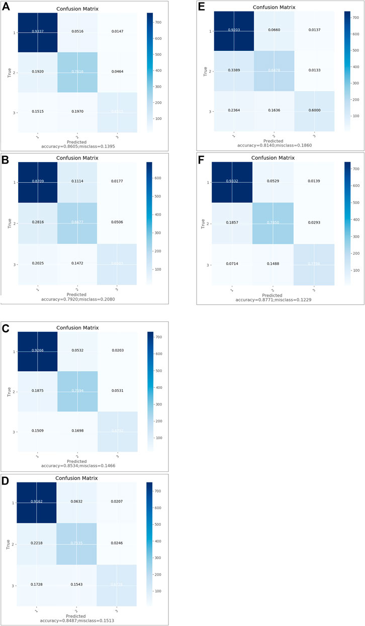
FIGURE 7. Normalized Confusion matrix of ML classifiers methods (A) RF, (B) ANN, (C) ADB, (D) XGB, (E) SVM, and (F) MLP used in the present study. The color variation represents the degree of normalisation and non-normalization as indicated by the data points on the color scale. Lithology code 1 indicates to shale, 2 indicates to sand, 3 indicates carbonate facies.

FIGURE 8

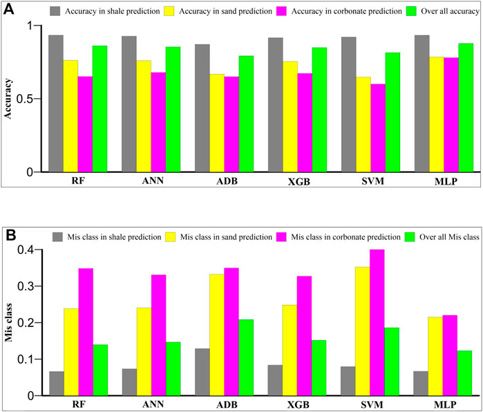
FIGURE 8. Outputs of each predictive model’s confusion matrix (A) accuracy and (B) misclass, computed for each litho-facies and overall, as well.

TABLE 4

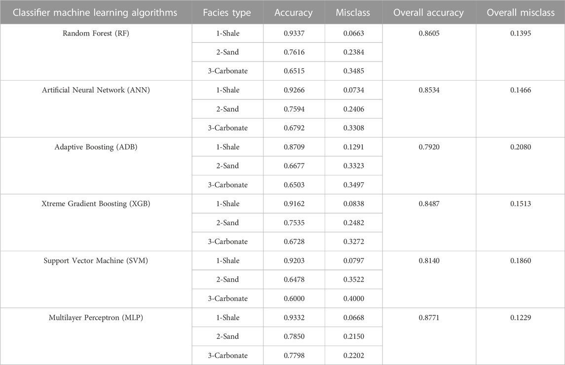
TABLE 4. Statistics, i.e., accuracy and misclass estimated in classification of shale sand and carbonate facies from different machine learning classifier algorithms.

Precision is the measure of correctly predicted litho-facies out of all litho-facies present in the log data. It also aids in measuring the model’s ability to classify true/actual litho-facies. It is found that the precision value ranges between 0.84 and 0.92 for shale facies, 0.65 to 0.78 for sand facies, and 0.82%–0.87% for the carbonate facies for all the models (Table 3). It is also noticed that the MLP, RF, ANN and XGB algorithms calculate considerably higher precision than the ADB and SVM in shale facies classification (Figure 6A). The MLP, RF and ANN algorithms calculate higher precision than the XGB, SVM and ADB in sand facies classification (Figure 6A). The MLP, SVM and XGB algorithms calculate higher precision than ADB, ANN and RF in carbonate facies classification (Figure 6A). Based on precision, the MLP method is the best-performing model, followed by the RF, ANN, XGB, SVM, and ADB methods in categorizing all three litho-facies.

Recall is the measure of the model correctly identifying the actual litho-facies as present in the log data. The recall tells us how many litho-facies we accurately predicted out of all of them. It is found that the recall value ranges between 0.87 and 0.93 for shale facies, 0.65 to 0.79 for sand facies, and 0.68 to 0.78 for the carbonate facies for all the models (Table 3). It is found that the RF, MLP, ANN, and SVM algorithms calculate higher recall values than the XGB and ADB in shale facies classification (Figure 6B). The MLP, RF, ANN, and XGB algorithms calculate higher precision than the ADB and SVM in sand facies classification (Figure 6B). The MLP, ANN, XGB, and RF algorithms calculate higher recall than the ADB and SVM in carbonate facies classification (Figure 6B). Based on recall, the MLP method is the best-performing method, followed by the ANN, XGB, RF, ADB, and SVM methods in categorizing all three litho-facies.

F1-score is the harmonic mean of the precision and recall value. High F1-score would indicate a high precision and recall value and can be used as a direct measure of the model’s efficacy in litho-facies classification. The F1-score value ranges between 0.86 and 0.93 for shale facies, 0.66 to 0.79 for sand facies, and 0.70 to 0.82 for the carbonate facies considering all the models (Table 3). It is found that the MLP, RF and ANN methods calculate a higher F1-score than the XGB, SVM and ADB methods in shale facies classification (Figure 6C). The MLP, RF and ANN methods calculate higher F1-score than the XGB, SVM and ADB in shale facies classification (Figure 6C). The MLP algorithm calculates a higher F1-score than the XGB, ANN, SVM, ADB and RF in carbonate facies classification (Figure 6C). Based on F1-score, the MLP method is the best-performing model, followed by the RF, ANN, XGB, SVM and ADB methods in determining all three litho-facies.

The confusion matrix (Figures 7A–F; Figures 8A,B) is a chart of actual and predicted results for an ML classifier determined by statistical parameters that are true positives, true negatives, false positives, and false negatives (Navin and Pankaja, 2016). The diagonal values of the confusion matrix indicate the true positives for each litho-facies. Accuracy and misclass are the most important parameters used in classification problems. Accuracy is calculated as the ratio of the correctly predicted and total records, whereas misclass is calculated by the one minus accuracy. The high accuracy value hints at a good agreement between the predicted and actual lithofacies. Accuracy values ranged between 0.871 and 0.934 for shale facies, 0.648 to 0.785 for sand facies, and 0.600 to 0.779 for the carbonate facies considering all the models (Table 4). It is found that the RF, MLP ANN, and SVM algorithms calculate higher accuracy in shale facies classification than the XGB and ADB methods (Figure 7A–F; Figure 8A, B). The MLP, RF, ANN, and XGB algorithms calculate higher accuracy than the ADB and SVM in sand facies classification (Figure 7A–F; Figure 8A, B). The MLP algorithm calculates considerably high accuracy in carbonate facies classification than the ANN, XGB, RF ADB, and SVM (Figure 7A–F; Figure 8A, B). Overall, the MLP model estimates maximum accuracy, followed by the RF, ANN, XGB, SVM, and ADB methods in classifying all three facies. Subsequently, the lowest misclass values were recorded for the MLP method, followed by the RF, ANN, XGB, SVM, and ADB methods. Based on accuracy and misclass values, the MLP method is again the best-performing method, followed by the RF, ANN, XGB, SVM, and ADB methods.

5.2 Lithological characterization of Mississauga and Abenaki Formation

We generated the facies volumes by applying the above-discussed ML methods on 3D seismic data. Figures 9A–F demonstrate the arbitrary line of litho-facies with three lithologies, essentially shale (1-grey), sand (2-yellow) and carbonate (3-pink), passing through both wells (B-41 and L-30). We noticed a good correlation between the predicted litho-facies and the overlaid well litho-facies strips. The arbitrary section determines the spatial and temporal distributions of the different litho-facies from time equivalent depth of 1,800 ms–3,000 ms (Figures 9A–F). The entire vertical succession considered in this study was deposited during Middle Jurassic to Middle Cretaceous geological period. Abenaki top, a broad carbonate platform formed, is the boundary of the Jurassic to the Cretaceous period.

FIGURE 9

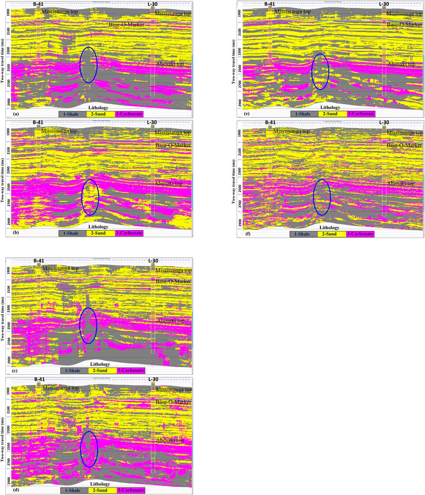
FIGURE 9. An arbitrary line section is passing through both wells as indicated extracted from the (A) RF, (B) ANN, (C) ADB, (D) XGB, (E) SVM, and (F) MLP facies volumes. Notice the good correlation between the predicted litho-facies and the well litho-facies strips overlaid.

Mississauga Formation mainly consists of sand facies with alternating shale and carbonate facies. All six methods’ results were in good agreement throughout the Mississauga Formation (Figures 9A–F). These sand facies were deposited in a deltaic environment and are widespread throughout the Scotian Basin. A change in tectonism most likely caused the altered Mississauga sedimentation during the separation of European and North American plates and regional sea-level rise (Jansa and Wade, 1975). Due to this reason, shale and carbonate facies were also found deposited in alternation. Previous researchers subdivided Abenaki Formation into four members, i.e., Scatarie, Misaine, Baccaro, and Artimon (McIver, 1972; Given, 1977; Eliuk, 1978; MacLean and Wade, 1993). The Artimon member is the top part of the Abenaki Formation, mainly characterized by carbonate and argillaceous facies. Baccaro member is dominated by carbonate facies deposited in the shallow marine environment. Below this member, Misaine member is dominated by the transgressive shale up to 200 m (Eliuk, 1978). Below Misaine member, Scatarie mainly consists of carbonate and shale facies. In the present study, carbonate facies from Artimon, Baccaro and Scatarie members, and shale facies from Misaine member were precisely delineated. Our results (Figures 9A–F) also agree with litho-facies away from the boreholes expected to be deposited in different depositional environments in the Penobscot field (refer to Figure 2).

We also noticed a few significant discrepancies from the arbitrary sections. First, we found the problem-related resolving capability of different methods; as a result, some methods estimate the litho-facies in chunks. Second, an anomalous zone (blue oval) was identified, showing different litho-facies in different methods. These discrepancies arise away from borehole locations, suggesting the validation of the predicted results.

6 Validation

Validation is an integral part of increasing confidence in a study’s findings. It can be done by comparing the findings of other complementary methods or using existing records. In the present research work, the estimated results from ML methods are validated by comparing them to the findings of the frequency and polarity attributes (Figures 10A, B), as explained below.

FIGURE 10

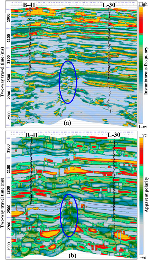
FIGURE 10. The results estimated from predicted litho-facies were validated with (A) Instantaneous frequency and (B) apparent polarity attributes.

6.1 Instantaneous frequency

Instantaneous frequency is a proven useful qualitative seismic attribute for determining stratigraphic terminations, thickness, and litho-facies changes (Taner et al., 1994; Castagna et al., 2003; Sukmono et al., 2006; Tai et al., 2009; Lu and Zhang, 2011). It is calculated as the time change rate of the instantaneous phase divided by 2π. In general, high-frequency responses signify dense formation (here, carbonate facies), while low-frequency responses signify loose formation (here, shale facies). Frequency values are also affected due to the intergranular pores (high-porosity) and the nature of the fluid present within them. Figure 10A depicts the arbitrary instantaneous frequency section passing through both wells. The entire section shows a significant frequency variation ranging between 7 and 50 Hz. It is found that chaotic and low (8 Hz) to high (42 Hz) frequency responses from the anomalous zone highlighted in Figures 9A–F. Based on frequency responses, the presence of all three litho-facies of thin and discrete nature is expected.

6.2 Apparent polarity

Polarity characteristics are a helpful tool in subsurface litho-facies delineation. Change in polarity value occurs due to change in impedance with depth (Brown, 1999; Barnes, 2006; Sukmono et al., 2006; Sukmono, 2010). The change in impedance indicates the change in litho-facies in the subsurface. Figure 10B depicts the arbitrary instantaneous frequency section passing through both wells. A constant apparent polarity marks the Abenaki top. As highlighted in Figure 6A–F; Figure 7A, the anomalous zone is characterized by a random apparent polarity response. It indicates the termination of Abenaki carbonate facies due to the possible inclusion of clastic facies (Figures 9A–F). The inferences drawn based on the polarity attribute are well corroborated with the observations from the frequency attribute (Figure 9A).

7 Discussion

A qualitative and quantitative attempt has been made to assess the accuracy of various ML classifier techniques in litho-facies discrimination. Calculated statistics (precision, recall, F1-score, accuracy and misclass) provide numerical inputs in the comparative evaluation of each ML model (Dixit and Mandal, 2020; Kumar et al., 2022; Srivardhan, 2022). Initially, three different litho-facies (shale, sand, and carbonate facies) were interpreted by analyzing different wireline logs from both wells. Further, these litho-facies were predicted throughout the 3D volume using seismic attributes as input features (Table 2) and litho-log from wells as target features. Previously, various scientists have successfully applied supervised and unsupervised ML methods on well logs and seismic data for litho-facies prediction (Wang and Carr, 2012; Bhattacharya et al., 2016; Zhang and Zhan, 2017; Chevitarese et al., 2018; Bressan et al., 2020; Liu et al., 2021; Xu et al., 2021; Babu et al., 2022). These studies were mostly applied two- or three-ML methods to interpret the lithological distribution in hydrocarbon and coal explorations. Here, we performed comparative assessment of 6 ML methods viz., RF, ANN, ADB, XGB, SVM, and MLP methods and evaluated their performance in litho-facies classifications in hydrocarbon exploration purposes.

To assess the model’s efficacy, we examined all the parameters (evaluation and confusion matrices) together. However, precision and recall are often in tension (precision increases, then recall decreases and vice-versa). Therefore, F1-score, the harmonic mean of the precision and recall, can be a reliable indicator of the model’s performance in various litho-facies classifications (Table 3; Figure 6C). Higher F1-score (0.86–0.92) values found on test data suggest that all six methods performed well in shale facies prediction. Relatively lower F1-score values were found in the estimation of carbonate facies (0.70–0.82) and sand facies (0.66–0.79). Accuracy and misclassification are the second major parameters to examine the models’ performance in litho-facies classification (Table 4; Figure 7A–F; Figure 8A, B). Relatively higher accuracy and lower misclass values were found for shale facies (0.87–0.94 and 0.06–0.13), followed by the sand facies (0.65–0.79 and 0.21–0.35) and the carbonate facies (0.60–0.78 and 0.22–0.40) considering all the models. Comparatively, the ML models’ accuracy score for specific lithologies varies significantly (Kumar et al., 2022). All the models efficiently classify the shale facies compared to the sand and carbonate facies. It indicates that the accuracy scores depend upon the number of samples (facies thickness) of shale, sand, and carbonate litho-facies used in test data.

In the current analysis, the ML models’ performance was found in order of MLP > RF > ANN > XGB > SVM > ADB for shale facies classification, MLP > RF > ANN > XGB > SVM > ADB for sand facies classification, and MLP >ANN >XGB >RF >SVM > ADB for carbonate facies classification. On an overall scale, the performance of ML models is in order of MLP > RF > ANN > XGB > SVM > ADB in the classification of all three litho-facies. A similar model performance order was also found from overall accuracy and misclass values in classifying all three litho-facies. Incorporating tuned regularization/penalty parameters in the MLP method is primarily responsible for improved results (Van der Baan and Jutten, 2000; Dixit and Mandal, 2020; Kumar et al., 2022). Due to a large number of trees, RF is an ensemble-based method that avoids overfitting and emerged as a powerful tool for classification. Xtreme Gradient Boosting emerged as a highly effective and accurate model by adding numerous trees in succession and focusing on the errors from the preceding one. Adaptive boosting algorithm uses empirical evidence and is highly susceptible to uniform noise, possibly making the model poorly performed in the present analysis. SVM classifiers are accurate, perform well in high-dimensional spaces, and need relatively less memory. However, the major problem associated with the SVM classifier is poorly handling the overlapping classes. On the other hand, several other factors affect the accuracy of the models. Relatively lower frequency bandwidth in seismic data caused the overlapping responses from different litho-facies, which caused the misclassification problem in facies estimation (Narayan et al., 2023). Models’ performance was also affected by delineating thin and discrete inter-bedded facies. Therefore, validation of estimated results is necessary to ascertain the accuracy of the prediction model. Our results agree with the results of comparative study from Srivardhan, (2022) and Kumar et al. (2022).

8 Conclusion

The present study highlights the efficacy of the machine learning methods, namely, RF, ANN, ADB, XGB, SVM, and MLP, in classifying the shale, sand and carbonate facies from the Penobscot field, Scotian Basin. These ML models were trained and validated on well-based interpreted litho-facies data. The performance of the ML models was examined on test data through the confusion matrix (accuracy and misclass) and evaluation matrix (precision, recall, F1-score). On the overall scale, the accuracy score suggests that all the models performed best in classifying the shale facies (87%–94%), followed by the sand (65%–79%) and carbonate facies (60%–78%), respectively. The accuracy scores found for different litho-facies also depend on the thickness of the litho-facies present in the subsurface. Different ML models’ performances were found in order of MLP > RF >ANN > XGB > SVM > ADB for shale facies, MLP > RF > ANN > XGB >SVM > ADB for sand facies and MLP > ANN > XGB > RF > SVM > ADB for carbonate facies classifications. In the current analysis, the MLP method emerged as the best-performing model, whereas the ADB method was the least-performing tool in classifying all three litho-facies from Late Jurassic to Cretaceous deposits in the Penobscot field. The estimated distribution of the different litho-facies was found to be in good agreement with the previous geological understandings and eustatic curve (sea-level changes) from Jurassic to Cretaceous period in this region.

Data availability statement

The original contributions presented in the study are included in the article/Supplementary Material, further inquiries can be directed to the corresponding author.

Author contributions

All authors listed have made a substantial, direct, and intellectual contribution to the work and approved it for publication.

Acknowledgments

Deep thanks and gratitude to the Researchers Supporting Project number (RSP 2023R351), King Saud University, Riyadh, Saudi Arabia for funding this research article.

Conflict of interest

Authors SA, SK, AC, employed by Oil and Natural Gas Corporation (ONGC).

The remaining authors declare that the research was conducted in the absence of any commercial or financial relationships that could be construed as a potential conflict of interest.

Publisher’s note

All claims expressed in this article are solely those of the authors and do not necessarily represent those of their affiliated organizations, or those of the publisher, the editors and the reviewers. Any product that may be evaluated in this article, or claim that may be made by its manufacturer, is not guaranteed or endorsed by the publisher.

References

Babu, M. N., Venkatesh, A., and Nair, R. R. (2022). Characterization of complex fluvial-deltaic deposits in Northeast India using Poisson impedance inversion and non-parametric statistical technique. Sci. Rep. 12, 16917. doi:10.1038/s41598-022-21444-5

PubMed Abstract | CrossRef Full Text | Google Scholar

Barnes, A. (2006). Too many seismic attributes? CSEG Rec. 31, 41–45.

Google Scholar

Bhatnagar, P., Bennett, C., Khoudaiberdiev, R., Lepard, S., and Verma, S. (2017). Seismic attribute illumination of a synthetic transfer zone. Seg. Tech. Program Expand. Abstr., 2112–2116. doi:10.1190/segam2017-17664850.1

CrossRef Full Text | Google Scholar

Bhattacharya, S., Carr, T. R., and Pal, M. (2016). Comparison of supervised and unsupervised approaches for mudstone lithofacies classification: Case studies from the Bakken and Mahantango-Marcellus Shale, USA. J. Nat. Gas. Sci. Eng. 33, 1119–1133. doi:10.1016/j.jngse.2016.04.055

CrossRef Full Text | Google Scholar

Breiman, L. (1996). Bagging predictors. Mach. Learn. 24 (2), 123–140. doi:10.1007/bf00058655

CrossRef Full Text | Google Scholar

Breiman, L. (2001). Random forests. Mach. Learn. 45 (1), 5–32. doi:10.1023/a:1010933404324

CrossRef Full Text | Google Scholar

Bressan, T. S., de Souza, M. K., Girelli, T. J., and Junior, F. C. (2020). Evaluation of machine learning methods for lithology classification using geophysical data learning methods for lithology classification using geophysical data. Comput. Geoscie. 139, 104475. doi:10.1016/j.cageo.2020.104475

CrossRef Full Text | Google Scholar

Brown, A. R. (1999). Interpretation of three-dimensional seismic data. 5th ed. Tulsa. OK.AAPG.

Google Scholar

Campbell, T. J., Richards, F. W. B., Silva, R. L., Wach, G., and Eliuk, L. S. (2015). Interpretation of the Penobscot 3D seismic volume using constrained sparse spike inversion, Sable sub-Basin, offshore Nova Scotia. Mar. Pet. Geol. 68, 73–93. doi:10.1016/j.marpetgeo.2015.08.009

CrossRef Full Text | Google Scholar

Castagna, J. P., Sun, S., and Siegfried, R. W. (2003). Instantaneous spectral analysis: Detection of low-frequency shadows associated with hydrocarbons. Lead. Edge 22, 120–127. doi:10.1190/1.1559038

CrossRef Full Text | Google Scholar

Chen, T., and Guestrin, C. (2016). “Xgboost: A scalable tree boosting system,” in Proceedings of the 22nd acm sigkdd International Conf. on Knowle. Disc. and Data Mining, San Francisco, CA, August 13 - 17, 2016 (Association for Computing Machinery), 785–794.

Google Scholar

Chevitarese, D. S., Szwarcman, D., Gama e Silva, R. M., and Vital Brazil, E. (2018). “Deep learning applied to seismic facies classification: A methodology for training,” in Saint Petersburg 2018, Saint Petersburg, Russia, April, 9-12, 2018.

CrossRef Full Text | Google Scholar

Dixit, A., and Mandal, A. (2020). Detection of gas chimney and its linkage with deep-seated reservoir in Poseidon, NW shelf, Australia from 3D seismic data using multi-attribute analysis and artificial neural network approach. J. Nat. Gas. Eng. 83, 103586. doi:10.1016/j.jngse.2020.103586

CrossRef Full Text | Google Scholar

Dramsch, J. S. (2020). 70 years of machine learning in geoscience in review. Adv. Geophys 61, 1–55. doi:10.1016/bs.agph.2020.08.002

CrossRef Full Text | Google Scholar

Eliuk, L. S., and Crevello, P. (1985). Upper jurassic and lower cretaceous deep-water build-ups, Abenaki Formation, nova scotia shelf. SEPM Soc. Sediment. Geol. 6. doi:10.2110/cor.85.06

CrossRef Full Text | Google Scholar

Eliuk, L. S. (1978). The Abenaki Formation, Nova Scotia Shelf, Canada--a depositional and diagenetic model for a Mesozoic carbonate platform. Bull. Can. Pet. Geol. 26, 424–514. doi:10.35767/gscpgbull.26.4.424

CrossRef Full Text | Google Scholar

Freund, Y., and Schapire, R. E. (1997). A decision-theoretic generalization of on-line learning and an application to boosting. J. Comput. Syst. Sci. 55 (1), 119–139. doi:10.1006/jcss.1997.1504

CrossRef Full Text | Google Scholar

Given, M. (1977). Mesozoic and early cenozoic geology of offshore nova scotia. Bull. Can. Petroleum Geol. 25, 63–91. doi:10.35767/gscpgbull.25.1.063

CrossRef Full Text | Google Scholar

Haq, B. U., Hardenbol, J., and Vail, P. R. (1987). Chronology of fluctuating sea levels since the triassic. Science 235, 1156–1167. doi:10.1126/science.235.4793.1156

PubMed Abstract | CrossRef Full Text | Google Scholar

Ho, T. K. (1995). “Random decision forests,” in Proceedings of 3rd International Conference on Document Analysis and Recognition, Montreal, Canada, 14-16 August 1995 (IEEE), 278–282.

Google Scholar

Jansa, L. F., Pratt, B. R., and Dromart, G. (1989). “Deep water thrombolite mounds from the upper Jurassic of offshore nova scotia Reefs, Canada, and Adjacent Area,” in Canadian soc. Of petrol. Geol. Memoir. Editors H. H. J. Geldsetzer, N. P. James, and G. E Tebbutt, 13, 725–735.

Google Scholar

Jansa, L. F., and Wade, J. A. (1975). Paleogeography and sedimentation in the mesozoic and cenozoic, southeastern Canada. Canada's continent. Margins and offshore petrol. Expl, 79–102.

Google Scholar

Keynejad, S., Sbar, M. L., and Johnson, R. A. (2019). Assessment of machine-learning techniques in predicting litho-fluid facies logs in hydrocarbon wells. Interpretation 7 (3), SF1–SF13. doi:10.1190/int-2018-0115.1

CrossRef Full Text | Google Scholar

Kidston, A. G., Brown, D. E., Smith, B. M., and Altheim, B. (2005). The upper jurassic Abenaki Formation offshore Nova Scotia. A seismic and geologic perspective: Canada-nova Scotia offshore petroleum board. Halifax: Nova Scotia, 21–26.

Google Scholar

Kumar, T., Seelam, N. K., and Srinivasa Rao, G. (2022). Lithology prediction from well log data using machine learning techniques: A case study from talcher coalfield, eastern India. J. Appl. Geophys. 199, 104605. doi:10.1016/j.jappgeo.2022.104605

CrossRef Full Text | Google Scholar

Liu, X., Ge, Q., Chen, X., Li, J., and Chen, Y. (2021). Extreme learning machine for multivariate reservoir characterization. J. Pet. Sci. Eng. 205, 108869. doi:10.1016/j.petrol.2021.108869

CrossRef Full Text | Google Scholar

Lu, W., and Zhang, C. K. (2011). “A robust instantaneous frequency estimation method,”. P093 In 73rd EAGE Conf. and Exhib. incorporating SPE EUROPEC, Vienna,, 23 May 2011 - 27 May 2011. doi:10.3997/2214-4609.20149432

CrossRef Full Text | Google Scholar

MacLean, B. C., and Wade, J. A. (1993). Seismic markers and stratigraphic picks in the Scotian Basin wells. East coast basin atlas series. Geol. Sur. Can., 276. doi:10.4095/221116

CrossRef Full Text | Google Scholar

MacLeod, N. (2019). Artificial intelligence and machine learning in the Earth sciences. Acta Geol. Sin. Engl. Ed.) 93, 48–51. doi:10.1111/1755-6724.14241

CrossRef Full Text | Google Scholar

Maurya, S. P. (2019). Estimating elastic impedance from seismic inversion method: A study from nova scotia field, Canada. Curr. Sci. 116, 628–725. doi:10.18520/cs/v116/i4/628-635

CrossRef Full Text | Google Scholar

McCormack, M. D. (1991). Neural computing in geophysics. Lead. Edge 10 (1), 11–15. doi:10.1190/1.1436771

CrossRef Full Text | Google Scholar

McIver, N. (1972). Cenozoic and mesozoic stratigraphy of the nova scotia shelf. Can. J. Earth Sci. 9, 54–70. doi:10.1139/e72-005

CrossRef Full Text | Google Scholar

Narayan, S., Sahoo, S. D., Kar, S., Pal, S. K., and Kangsabanik, S. (2023). Improved reservoir characterization by means of supervised machine learning and model-based seismic impedance inversion in the Penobscot field, Scotian Basin. Energy Geos, 100180. doi:10.1016/j.engeos.2023.100180

CrossRef Full Text | Google Scholar

Navin, J. R. M., and Pankaja, R. (2016). Performance analysis of text classification algorithms using confusion matrix. Int. J. Eng. Tech. Res. 6 (4), 2321–0869.

Google Scholar

NSDE (Nova Scotia Department of Energy) (2011). Play fairway analysis atlas-offshore Nova Scotia, Canada. Available at: http://energy.novascotia.ca/oil-and-gas/offshore/play-fairway analysis/analysis.

Google Scholar

Ray, A. K., Khoudaiberdiev, R., Bennett, C., Bhatnagar, P., Boruah, A., Dandapani, R., et al. (2022). Attribute-assisted interpretation of deltaic channel system using enhanced 3D seismic data, offshore Nova Scotia. J. Nat. Gas Sci. Eng. Doi.org/ 99, 104428. doi:10.1016/j.jngse.2022.104428

CrossRef Full Text | Google Scholar

Schmitt, P., Veronez, M. R., Tognoli, F. M. W., Todt, V., Lopes, R. C., and Silva, C. A. U. (2013). Electro facies modelling and lithological classification of coals and mud bearing ingrained siliciclastic rocks based on neural networks. Earth Sci. Res. 2, 193–208. doi:10.5539/esr.v2n1p193

CrossRef Full Text | Google Scholar

Srivardhan, V. (2022). Adaptive boosting of random forest algorithm for automatic petrophysical interpretation of well logs petrophysical interpretation of well logs. Acta Geod. Geophys. 57, 495–508. doi:10.1007/s40328-022-00385-5

CrossRef Full Text | Google Scholar

Sukmono, S. (2010). “Fundamental issues on the application of seismic methodologies for carbonate reservoir characterization,” in Proceed. Indonesian Petrol. Assoc. 34th Annual Convention and Exhibition, Jakarta, 18-20 May 2010.

Google Scholar

Sukmono, S., Samodra, A., SardjitoWaluyo, W., and Tjiptoharsono, S. (2006). Integrating seismic attributes for reservoir characterization in Melandong Field, Indonesia. Lead. Edge 25 (5), 532–538. doi:10.1190/1.2202653

CrossRef Full Text | Google Scholar

Sun, Z., Jiang, B., Li, X., Li, J., and Xiao, K. (2020). A data-driven approach for lithology identification based on parameter-optimized ensemble learning identification based on parameter-optimized ensemble learning. Energies 13 (15), 3903. doi:10.3390/en13153903

CrossRef Full Text | Google Scholar

Tai, S., Puryear, C., and Castagna, J. P. (2009). “Local frequency as a direct hydrocarbon indicator,”. Presented at the SEG Technical Program Expanded Abstracts 2009 in SEG technical program expanded abstracts 2009 (Tulsa: SEG), 2160–2164. doi:10.1190/1.3255284

CrossRef Full Text | Google Scholar

Taner, M. T., Schuelke, J. S., O'Doherty, R., and Baysal, E. (1994). “Seismic attributes revisited,” in 64th Annual Int. Meeting Soc. of Expl. Geophys. Exp. Abst., Los Angeles, CA, 23 October 1994 (SEG), 1104–1106.

CrossRef Full Text | Google Scholar

Van der Baan, M., and Jutten, C. (2000). Neural networks in geophysical applications. Geophysics 65 (4), 1032–1047. doi:10.1190/1.1444797

CrossRef Full Text | Google Scholar

Vapnik, V. N. (1995). The nature of statistical learning theory. New York, NY: Springer.

Google Scholar

Wade, J. A., MacLean, B. C., and Williams, G. L. (1995). Mesozoic and cenozoic stratigraphy, eastern scotian shelf: New interpretations. Can. J. Earth Sci. 32, 1462–1473. doi:10.1139/e95-118

CrossRef Full Text | Google Scholar

Wang, G., and Carr, T. R. (2012). Methodology of organic-rich shale lithofacies identification and prediction: A case study from marcellus shale in the appalachian basin and prediction: A case study from marcellus shale in the appalachian basin. Comput. Geoscie. 49, 151–163. doi:10.1016/j.cageo.2012.07.011

CrossRef Full Text | Google Scholar

Weissenberger, J. A., Wierzbicki, R. A., and Harland, N. J. (2006). Carbonate sequence stratigraphy and petroleum geology of the Jurassic deep Panuke field. Canada: Offshore Nova Scotia.

Google Scholar

Xu, Z., Shi, H., Lin, P., and Liu, T. (2021). Integrated lithology identification based on images and elemental data from rocks and elemental data from rocks. J. Pet. Sci. Eng. 205, 108853. doi:10.1016/j.petrol.2021.108853

CrossRef Full Text | Google Scholar

Zhang, L., and Zhan, C. (2017). “Machine learning in rock facies classification - an application of XGBoost,” in Int. Geophys. Conf. Qingdao, Qingdao, China, 17-20 April 2017 (SEG).

CrossRef Full Text | Google Scholar