A modified symplectic discontinuous Galerkin method for acoustic and elastic wave simulations

Numerically solving seismic wave equations is vital to large-scale forward modeling and full waveform inversion. In this paper, a new modified symplectic discontinuous Galerkin (MSDG) method is proposed to solve the acoustic and elastic equations. The MSDG method employs a symmetric interior penalty Galerkin formulation as the space discretization. The time discretization is based on a modified symplectic partitioned Runge–Kutta scheme with minimized phase error. Thus, the MSDG method has the advantages of high accuracy, being flexible to deal with complex geometric boundaries and internal structures, and stable for long time simulations. The numerical stability conditions, dispersion and dissipation are investigated in detail for the MSDG method. To validate the method, we carry out several numerical examples for solving the acoustic and elastic wave equations in various media. The numerical results show that the MSDG method can effectively suppress the numerical dispersion and is suitable for wavefield simulations.

1 Introduction

Nowadays, full waveform inversion (FWI) is one of the important techniques to study underground structures, which has been widely used in geophysical exploration (Tarantola, 1984). FWI is essentially an optimization problem, the main goal of which is to minimize the error between the observed waveform or travel time records and the synthetic data. The synthetic data are mainly obtained by forward modeling. Therefore, the accuracy of FWI strongly depends on the accuracy of forward modeling. A high-precision forward-modeling method can greatly reduce the computation and storage requirements in FWI. Many numerical algorithms have been developed, such as the finite difference method (e.g., Dablain, 1986; Virieux, 1986; Yang et al., 2003; Liu and Sen, 2009; Igel, 2017), finite element method (Chen, 1984; Yang, 2002; Meng and Fu, 2017), pseudo-spectral method (Kosloff et al., 1982; Fornberg, 1998), and spectral element method (Komatitsch and Vilotte, 1998; Tong et al., 2014; Liu et al., 2017). These methods have their own advantages as well as drawbacks. For instance, the finite difference method has advantages of convenient programming, small storage capacity and fast calculation speed, but it usually generates serious numerical dispersion in case of coarse grids (e.g., Sei and Symes et al., 1995; Ma et al., 2011; Yang et al., 2007; Yang et al., 2012), and the finite difference method cannot flexibly deal with the complex geometric structures.

In recent years, the discontinuous Galerkin (DG) methods have gained increasingly attention in computational geophysics. The DG method has many advantages, such as high precision, flexible handling of complex geometric boundaries and boundary conditions, easy parallel calculation, small numerical dispersion, etc. It is precisely because of these advantages that much research work has been carried out on the DG methods (e.g., Cockburn and Shu, 2001; Li, 2006). Among them, there are also many studies on solving wave propagation problems (e.g., Käser and Dumbser, 2006; Rivière, 2008; Etienne et al., 2010; Wilcox et al., 2010; Yang et al., 2016; Ferroni et al., 2017; Meng and Fu, 2018; He et al., 2019; He et al., 2020a, 2020b; He X. J. et al., 2022, He et al., 2022 X.).

DG methods can be divided into two categories when dealing with boundary integrals: the flux-based DG method and interior penalty DG method. This paper concentrates on the latter, which adds a penalty term to the boundary integral. This method was originally proposed by Rivière and Wheeler (2003) to solve the scalar acoustic wave propagation problems. They proposed a non-symmetric internal penalty Galerkin method. Afterwards, Dawson et al. (2004) continued to carry out a series of analyses on the penalty terms. Grote (2006) suggested a symmetric penalty term in the DG spatial discretization. All the methods mentioned above are used in computational geophysics. The numerical properties of the interior penalty DG method for solving scalar wave equation were first analyzed by Ainsworth et al. (2006). They also discussed the choice of penalty function. Detailed analyses of the numerical stability, numerical dispersion and dissipation for solving elastic equations were carried out by de Basabe et al. (2008) and de Basabe and Sen (2010). The above analyses are limited to 1D and 2D. Ferroni et al. (2017) generalized the analysis to 3D case, and they also compared the hexahedral mesh with the tetrahedral mesh.

For numerically solving wave equations, traditional time discretization methods usually introduce artificial dissipation, which leads to changes in system conservation quantities such as energy in long-term calculations. The symplectic time-stepping method is constructed based on the Hamiltonian mechanics system, which does not introduce artificial dissipation, so it is especially suitable for long-time simulations. Many symplectic time-stepping methods have emerged. (Hairer et al., 2006; Chen, 2009; Iwatsu, 2009; Feng and Qin, 2010; Liu et al., 2017; Ma et al., 2017; He et al., 2019). Particularly, Ma and Yang (2017) investigated the symplectic schemes, and suggested a series of modified symplectic partitioned Runge–Kutta methods, and their results suggest that these modified schemes have minimized phase errors. Moreover, they conducted a numerical test on phase accuracy after long-time simulations, and found that the modified symplectic partitioned Runge–Kutta methods are more stable than traditional methods.

This research is an advance based on the work of He et al. (2019), in which they used a classic symplectic partitioned Runge–Kutta method proposed by Iwatsu (2009), and they only considered the acoustic wave equation. In this study, a modified symplectic discontinuous Galerkin (MSDG) method is proposed for seismic wavefield modeling, which combines the interior penalty DG method with a modified third-order partitioned Runge–Kutta method proposed by Ma and Yang (2017). We first outline the discontinuous Galerkin and time-stepping formulations, then we investigate the stability condition, dispersion and dissipation in detail. Finally, several numerical examples are presented to validate the MSDG method.

2 Scheme

2.1 Space discretization

We first consider the spatial discretization of interior penalty DG method for the acoustic case. The governing equation can be written as:

${\lambda }^{-1}{p}_{tt}-\nabla \cdot \left({\rho }^{-1}\nabla p\right)=f(1)$

where p denotes the wave displacement, λ is the Lamé parameter, ρ is the density, $\nabla$ is the gradient operator, and f is the external source. The acoustic velocity c is computed as: $c=\sqrt{\lambda /\rho }$. Let $\mathrm{\Omega }\in {\mathbb{R}}^2$ be the computational domain. We consider a non-overlapping partition of $\mathrm{\Omega }$ and denote it by ${\mathrm{\Omega }}_h$. The partition ${\mathrm{\Omega }}_h$ is composed of quadrangular or triangular elements denoted by $\left\{{\mathrm{\Omega }}_i\right\}$. The union of all element boundaries is denoted by ${\mathrm{\Gamma }}_h$. The polynomial space with degree no more than κ is denoted by P^κ. We then consider the following test function space:

$V_h=\left\{q\in L^2\left(\mathrm{\Omega }\right):q{|}_E\in P^{\kappa }\left(E\right),\forall E\in {\mathrm{\Omega }}_h\right\}(2)$

As can be seen in Eq. 2 that the test function q is allowed to be discontinuous across element interfaces.

We then multiply Eq. 1 with a test function q, and integrate on Ω. By applying the divergence theorem, the following equation can be obtained:

${\int }_{\mathrm{\Omega }}{\lambda }^{-1}{p}_{tt}\cdot q\mathrm{d}V+{\int }_{\mathrm{\Omega }}{\rho }^{-1}\nabla p\cdot \nabla q\mathrm{d}V-{\displaystyle \sum _{F\in {\mathrm{\Gamma }}_h}}{\int }_F{\rho }^{-1}\left(\mathbf{n}\cdot \nabla p\right)q\mathrm{d}\mathrm{s}={\int }_{\mathrm{\Omega }}f\cdot q\mathrm{d}V(3)$

in which $F\in \partial E$ is the interfaces involved in ${\mathrm{\Gamma }}_h$, and n refers to a normal vector on F. We define two notations $p^{+}$ and $p^{-}$ to represent the traces of p taken from internal and external of E, respectively. Accordingly, we define two opposite normal vectors ${\mathbf{n}}^{+}$ and ${\mathbf{n}}^{-}$ with ${\mathbf{n}}^{+}$ = ${\mathbf{n}}^{-}$. Then, following the notations in Grote et al. (2006), de Basabe et al. (2008) and de Basabe and Sen (2010), we can define the average operator {} and the jump operator [] as:

$\left[p\right]:=p^{+}-p^{-},\left\{p\right\}:=\frac{1}{2}\left(p^{+}+p^{-}\right)(4)$

Following the theory of the interior penalty DG method, Eq. 3 can be rewritten as:

${\displaystyle \sum _{E\in {\mathrm{\Omega }}_h}}{\int }_E{\lambda }^{-1}{p}_{tt}\cdot q\mathrm{d}V+{\displaystyle \sum _{E\in {\mathrm{\Omega }}_h}}{\int }_E{\rho }^{-1}\nabla q\cdot \nabla p\mathrm{d}V+{\displaystyle \sum _{F\in {\mathrm{\Gamma }}_h}}{J}_F\left(p,q;\gamma \right)={\displaystyle \sum _{E\in {\mathrm{\Omega }}_h}}{\int }_{E}f\cdot q\mathrm{d}V(5)$

where the term $J_F$ is defined as:

$J_F\left(u,v;\gamma \right)=-\underset{F}{{\displaystyle \int }}\left[q\right]\cdot \left\{\mathbf{n}\cdot {\rho }^{-1}\nabla p\right\}\mathrm{d}\mathrm{s}-\underset{F}{{\displaystyle \int }}\left[p\right]\cdot \left\{\mathbf{n}\cdot {\rho }^{-1}\nabla q\right\}\mathrm{d}\mathrm{s}+\gamma \underset{F}{{\displaystyle \int }}\left\{{\rho }^{-1}\right\}\cdot \left[p\right]\cdot \left[q\right]\mathrm{d}\mathrm{s}.(6)$

In Eq. 5, the parameter $\gamma$ is related to the penalty term. In actual computation, we can use $\gamma =\left(\kappa +1\right)\left(\kappa +2\right)/2r$, where r is the length of the edge. The method in Eqs. 5, 6 is also called the symmetric interior penalty DG method Grote (2006).

Let ${\left\{{\phi }_{\left.i\right|E}\right\}}_{i=1}^{d_{\mathit{l}\mathit{o}\mathit{c}}}$ be a basis function series that is only related to space but independent of time, where $d_{\mathit{l}\mathit{o}\mathit{c}}$ denotes the number of basis functions. There are many choices for ${\left\{{\phi }_{\left.i\right|E}\right\}}_{i=1}^{d_{\mathit{l}\mathit{o}\mathit{c}}}$ (Cockburn and Shu, 2001; de Basabe et al., 2008; Rivière, 2008), any of which can be used. We now consider the basis function expansion of Eq. 5. We first write the wave displacement p as $p={\displaystyle \sum _{i=1}^{d_{\mathit{l}\mathit{o}\mathit{c}}}}{p}_i\left(t\right){\phi }_i$, where ${\left\{p_i\left(t\right)\right\}}_{i=1}^{d_{\mathit{l}\mathit{o}\mathit{c}}}$ are the unknow coefficients. Then, we substitute the expansion of p into Eq. 5. An ordinary differential equation (ODE) system can be obtained (He et al., 2019):

$M_{ij}{\partial }_{tt}{p}_j+N_{ij}{p}_j+J_{ij}{p}_j={\widehat{F}}_i(7)$

where:

$\begin{array}{l}{M}_{ij}={\displaystyle \sum _{E\in {\mathrm{\Omega }}_h}}{\int }_E{\lambda }^{-1}{\phi }_j\cdot {\phi }_i\mathrm{d}V,\hspace{1em}{N}_{ij}={\displaystyle \sum _{E\in {\mathrm{\Omega }}_h}}{\int }_E{\rho }^{-1}\nabla {\phi }_j\cdot \nabla {\phi }_i\mathrm{d}V,\\ J_{ij}={\displaystyle \sum _{F\in {\mathrm{\Gamma }}_h}}{J}_F\left({\phi }_j,{\phi }_i;\eta ,\gamma \right),\hspace{1em}{\widehat{F}}_i={\displaystyle \sum _{E\in {\mathrm{\Omega }}_h}}{\int }_{E}f\cdot {\phi }_i\mathrm{d}V,i,j=1,\dots ,d_{\mathit{l}\mathit{o}\mathit{c}}.\end{array}(8)$

Next, we introduce the interior penalty DG scheme for the elastic equations. We first consider a more general form of 2D P-SV wave equations:

$\left(\begin{array}{l}\rho \frac{{\partial }^2{u}_1}{\partial t^2}\\ \rho \frac{{\partial }^2{u}_3}{\partial t^2}\end{array}\right)-\nabla \cdot \left(\begin{array}{cc}{c}_{11}\frac{\partial u_1}{\partial x}+c_{13}\frac{\partial u_3}{\partial z}& c_{55}\frac{\partial u_1}{\partial z}+c_{55}\frac{\partial u_3}{\partial x}\\ c_{55}\frac{\partial u_1}{\partial z}+c_{55}\frac{\partial u_3}{\partial x}& c_{13}\frac{\partial u_1}{\partial x}+c_{33}\frac{\partial u_3}{\partial z}\end{array}\right)=\left(\begin{array}{l}{f}_1\\ f_2\end{array}\right)(9)$

where $c_{11},c_{13},c_{33},c_{55}$ are elastic parameters. In fact, Eq. 9 can represent the wave propagation in general anisotropic vertical transversely isotropic media. To simplify the expression, we introduce the following notation:

$\mathbf{u}={\left(u_1,u_3\right)}^T,\mathbf{f}={\left(f_1,f_2\right)}^T,\mathbf{\sigma }\left(\mathbf{u}\right)=\left(\begin{array}{cc}{c}_{11}\frac{\partial u_1}{\partial x}+c_{13}\frac{\partial u_3}{\partial z}& c_{55}\frac{\partial u_1}{\partial z}+c_{55}\frac{\partial u_3}{\partial x}\\ c_{55}\frac{\partial u_1}{\partial z}+c_{55}\frac{\partial u_3}{\partial x}& c_{13}\frac{\partial u_1}{\partial x}+c_{33}\frac{\partial u_3}{\partial z}\end{array}\right)(10)$

then, Eq. 9 can be recast as:

$\rho {\mathbf{u}}_{tt}-\nabla \cdot \mathbf{\sigma }\left(\mathbf{u}\right)=\mathbf{f}(11)$

We then multiply Eq. 11 with a test function vector v, and integrate over Ω. By applying the divergence theorem and the theory of the interior penalty DG method, we obtain:

${\displaystyle \sum _{E\in {\mathrm{\Omega }}_h}}{\int }_E\rho {\mathbf{u}}_{tt}\cdot \mathbf{v}\mathrm{d}V+{\displaystyle \sum _{E\in {\mathrm{\Omega }}_h}}{\int }_E\mathbf{\sigma }\cdot \nabla \mathbf{v}\mathrm{d}V+{\displaystyle \sum _{F\in {\mathrm{\Gamma }}_h}}{J}_F\left(\mathbf{u},\mathbf{v};\gamma \right)={\displaystyle \sum _{E\in {\mathrm{\Omega }}_h}}{\int }_E\mathbf{f}\cdot \mathbf{v}\mathrm{d}V(12)$

where the term $J_F$ is now defined as:

$J_F\left(\mathbf{u},\mathbf{v};\gamma \right)=-{\int }_F\left[\mathbf{v}\right]\cdot \left\{\mathbf{n}\cdot \mathbf{\sigma }\left(\mathbf{u}\right)\right\}\mathrm{d}\mathrm{s}-{\int }_F\left[\mathbf{u}\right]\cdot \left\{\mathbf{n}\cdot \mathbf{\sigma }\left(\mathbf{v}\right)\right\}\mathrm{d}\mathrm{s}+\gamma {\int }_F\left[\mathbf{u}\right]\cdot \left[\mathbf{v}\right]\mathrm{d}\mathrm{s}(13)$

For the basis function expansion of Eq. 12 in the case of elastic waves, the reader can follow the derivation for the case of acoustic wave. We can obtain an ODE system similar to Eq. 7. Here we omit the detailed derivation and description in order to avoid redundant narration.

2.2 Time discretization

We now continue to discretize the equations in time. To simplify the notations, a vector P is introduced to represent all the unknown coefficients. Then, Eq. 7 can be written as:

${\mathbf{P}}_{tt}=L\left(\mathbf{P}\right)+\widehat{\mathbf{F}}(14)$

where L is an operator related to the space discretization of interior penalty DG method.

To implement the partitioned Runge–Kutta time-stepping method, we first introduce an auxiliary intermediate vector V, which is defined as: $\mathbf{V}={\mathbf{P}}_t$. Then we can obtain the following system:

$\left\{\begin{array}{l}{\mathbf{P}}_t=\mathbf{V}\\ {\mathbf{V}}_t=L\left(\mathbf{P}\right)+\widehat{\mathbf{F}}\end{array}\right.(15)$

Afterwards, a modified third-order partitioned Runge–Kutta method proposed by Ma and Yang (2017) is employed to implement the time discretization, which reads:

$\left\{\begin{array}{l}{\mathbf{V}}_1={\mathbf{V}}^n+c_1\Delta t\left(L\left({\mathbf{P}}^n\right)+{\widehat{\mathbf{F}}}^n\right)\\ {\mathbf{P}}_1={\mathbf{P}}^n+d_1\Delta t{\mathbf{V}}_1\\ {\mathbf{V}}_2={\mathbf{V}}_1+c_2\Delta tL\left({\mathbf{P}}_1\right)\\ {\mathbf{P}}_2={\mathbf{P}}_1+d_2\Delta t{\mathbf{V}}_2\\ {\mathbf{V}}^{n+1}={\mathbf{V}}_2+c_3\Delta tL\left({\mathbf{P}}_2\right)\\ {\mathbf{P}}^{n+1}={\mathbf{P}}_2+d_3\Delta t{\mathbf{V}}^{n+1}\end{array}\right.(16)$

where the coefficients are:

$\left\{\begin{array}{l}{c}_1=0.46329510533007323\\ c_2=-0.09414279831674241\\ c_3=0.6308476929866692\\ d_1=-0.3544544907366482\\ d_2=1.0941427983167424\\ d_3=0.2603116924199058\end{array}\right.(17)$

Theoretical analyses and numerical test show that scheme of Eqs. 16, 17 has small phase errors and the phase accuracy can be maintained during long time simulation. Combining the temporal discretization introduced here with the space discretization, we obtain the MSDG method.

For the purpose of comparison, we also introduce two classic third-order time-stepping methods. The first is the symplectic third-order Runge–Kutta method proposed by Iwatsu (2009), which has the similar form as Eq. 16 but with the following different coefficients:

$\begin{array}{l}{c}_1=\frac{1}{12}\left(\sqrt{209/2}-7\right),c_2=\frac{11}{12},c_3=\frac{1}{12}\left(8-\sqrt{209/2}\right),\\ d_1=\frac{2}{9}\left(1+\sqrt{38/11}\right),d_2=\frac{2}{9}\left(1-\sqrt{38/11}\right),d_3=\frac{5}{9}.\end{array}(18)$

Incorporated with the interior penalty DG method in Section 2.1, we call this method the symplectic DG (SDG) method. He et al. (2019) studied this method in great detail.

The other is the classical three-order Runge–Kutta method proposed by Williamson (1980), which is:

$\begin{array}{l}{\mathbf{y}}_t:={\left(\begin{array}{l}\mathbf{P}\\ \mathbf{V}\end{array}\right)}_t=\left(\begin{array}{c}\mathbf{V}\\ \begin{array}{l}L\left(\mathbf{P}\right)+\widehat{\mathbf{F}}\end{array}\end{array}\right)=:g\left(t,\mathbf{y}\right),\\ \left\{\begin{array}{l}{\mathbf{y}}^{n+1}={\mathbf{y}}^n+\frac{\Delta t}{6}\left({\mathbf{W}}_1+4{\mathbf{W}}_2+{\mathbf{W}}_3\right)\\ {\mathbf{W}}_1=g\left(t^n,{\mathbf{y}}^n\right)\\ {\mathbf{W}}_2=g\left(t^n+\frac{\Delta t}{2},{\mathbf{y}}^n+\frac{\Delta t}{2}{\mathbf{W}}_1\right)\\ {\mathbf{W}}_3=g\left(t^n+\Delta t,{\mathbf{y}}^n-\Delta t{\mathbf{W}}_1+2\Delta t{\mathbf{W}}_2\right)\end{array}\right.\end{array}(19)$

Similarly, incorporated with the interior penalty DG method in Section 2.1, we name this method the classic DG (CDG) method.

3 Numerical properties

To discuss the numerical properties including the stability condition, dispersion and dissipation, plane wave analysis should be carried out first. Many studies have focused on the plane wave analysis of the interior penalty DG method for acoustic and elastic cases (e.g., Ainsworth et al., 2006; de Basabe and Sen, 2010; Ferroni et al., 2017; He et al., 2019; He et al., 2020a). One can follow the steps in the above listed studies to analyze the numerical properties of MSDG method. Here, we do not show the details of derivation, but only present the relevant results for the scalar wave equation in isotropic case. The results are based on the uniform rectangular elements and employ Gauss-Legendre polynomials as basis functions (Cockburn and Shu, 2001).

3.1 Stability conditions

Satisfying the numerical stability condition is an essential prerequisite for a numerical algorithm to keep the calculation stable. Typically, the numerical stability condition is given by the constraint relationship among wave speed c and the spatial and temporal steps h and $∆t$, known as the Courant–Friedrichs–Lewy (CFL) condition, which reads:

$c\frac{\Delta t}{h}\le {\alpha }_{\max }(20)$

where α_max is the maximum Courant number.

We study the numerical stability of the MSDG method and list the maximum Courant numbers in Table 1 for P^κ with κ = 1∼4. For comparison, the maximum Courant numbers for the CDG and SDG methods are also presented, which are obtained directly from the studies by He et al. (2019). From Table 1, we see that as κ increases, the maximum Courant numbers decreases significantly. We also observe that the maximum Courant number for the MSDG method is larger than that of SDG method, and the maximum Courant number of the CDG method is the smallest. Particularly, the maximum Courant number for the MSDG method have a 3% increase compared to the SDG method, and a 59% increase compared to the CDG method. The stability analyses show that the proposed MSDG method has superiority over traditional methods.

TABLE 1

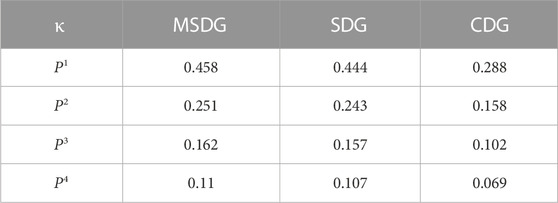
TABLE 1. The maximum Courant numbers for the MSDG, SDG and CDG methods.

3.2 Dispersion and dissipation

When we discretize the wave equation in space and time, numerical dispersion and dissipation usually appear. Here, we define the numerical dispersion R by the ratio between the numerical speed and the true speed. We also use the ratio of a numerical amplitude to the true amplitude to denote the numerical dissipation S. According to the definitions, closer values of R and S to 1 indicate smaller dispersion and dissipation, meaning a better numerical method. Generally, R and S are related to the spatial sampling ratio S_p, the Courant number $\alpha =c∆t/h$, as well as the direction of wave propagation θ. In the following analysis, the Courant number α is set to 0.1 for κ = 1∼3, α is 0.05 for κ= 4. This measure can guarantee that for all methods α is within the maximum Courant number. We also assume that the spatial sampling ratio S_p ≈ 0.4.

Figure 1 exhibits the numerical dispersion R of the MSDG method changing with propagation direction θ for κ = 1∼4. The results of the SDG and CDG methods are also presented for comparison. It is obvious that R decreases as κ increases. Moreover, R varies with the value of θ, meaning that the numerical dispersion has anisotropic character. Figure 1 also indicates that the values of R for these three methods are similar when κ = 1, 2; however, when κ = 3, 4, the values of R for CDG are obviously larger than that of MSDG and SDG, meaning that using symplectic Runge-Kutta time-stepping method has certain advantages over non-symplectic scheme. For MSDG and SDG methods, we observe some minor differences. Figure 1B shows that the numerical dispersion of MSDG is slightly smaller than that of SDG, demonstrating the slight advantage of MSDG method in numerical dispersion.

FIGURE 1

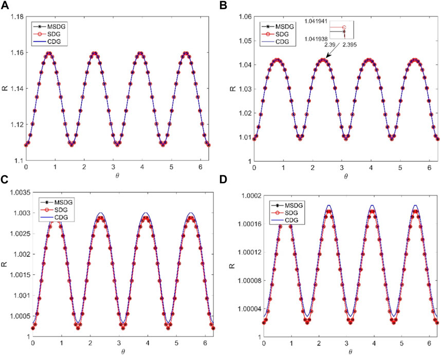
FIGURE 1. Numerical dispersion changing with the propagation direction. (A–D): κ = 1∼ 4.

Figure 2 shows the variation of numerical dissipation S. The anisotropy along with the propagation direction can also be identified. Unlike the case of numerical dispersion, the numerical dissipation of the three methods is quite different. Both MSDG and SDG methods do not introduce numerical dissipation, indicating that these two methods can maintain energy conservation and are beneficial to long-term simulations. However, the CDG method introduces a large numerical dissipation, indicating that the energy will attenuate in the wave propagation, which is not conducive to long-term simulation. The results of the numerical dissipation analysis fully illustrate the importance of adopting the symplectic scheme.

FIGURE 2

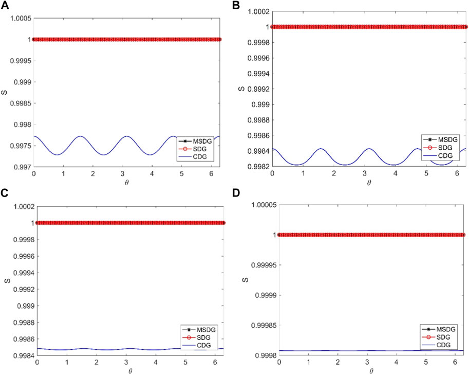
FIGURE 2. Numerical dissipation changing with the propagation direction. (A–D): κ = 1∼ 4.

4 Numerical examples

We now carry out several tests to illustrate the validity and efficiency of the proposed algorithm.

4.1 The acoustic model with long time simulation test

In the first example, the computational domain is a square with $0\le x,z\le 6$ km. The domain is discretized with uniform rectangles with 21.7 m × 21.7 m. The acoustic speed is 3 km/s. A point source is set at (3.0 km, 3.0 km), and its evolution equation is:

$f\left(t\right)=-5.76f_0^2\left[1-16{\left(0.6f_{0}t-1\right)}^2\right]\exp \left[-8{\left(0.6f_{0}t-1\right)}^2\right](21)$

where f₀ = 20 Hz. A receiver is set at (4.26 km, 4.26 km) to record the waveforms. We use a MSDG method with order κ = 2 of the basis function. The time increment is ∆t = 1.138 ms. We do not make any special treatment to the boundary conditions, and we just implement the simplest Dirichlet zero boundary condition.

We show the wavefield snapshot at t = 0.8 s in Figure 3A, from which we observe clear wave fronts without visible numerical dispersion. We also plot the normalized waveforms in the time interval of [0 s, 1.4 s] in Figure 3B. The solid line is the numerical result generated by the MSDG method, and the dotted line is the analytical result using Cagnidard-de Hoop algorithm (de Hoop, 1960). Comparing the two solutions, we find that they fit well, illustrating the correctness of our method. In addition, the waveforms exhibit no visible pseudo fluctuations, demonstrating the availability of our method for restraining the numerical dispersion.

FIGURE 3

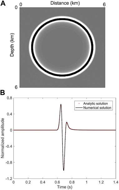
FIGURE 3. (A) Snapshots of the acoustic wavefields at t = 0.8 s, and (B) normalized waveform records in [0 s, 1.4 s] computed by the MSDG method in homogeneous acoustic medium.

Next, we intend to examine the long-time simulation capability of our method. We first plot the snapshots of the acoustic wavefields generated by the MSDG and CDG methods at t = 2 s in Figure 4A, where the left part is generated by the MSDG method and the right part is generated by the CDG method. The arrow indicates that there is a slight phase shift. To illustrate the performance of the two methods more clearly, we extend the simulation time to 13 s. Now the total time iteration steps is 11427. Figure 4B shows part of the waveform records in [11 s, 13 s]. The records produced by the CDG method are provided as well for comparison. The solutions obtained by reducing the time step by half for both methods are taken as two reference solutions, which show more accurate results. It is indicated that although the general waveform trends of these methods are consistent, there are subtle differences. Figure 5 gives closer observations of the waveforms in time intervals of [12.27 s, 12.31 s] and [12.86 s, 12.90 s], from which we clearly see that the CDG method provides the worst results, with significant deviations in phase and amplitude compared to the other results, whereas the results of MSDG method are close to the other two reference solutions. This experiment demonstrates the effectiveness and reliability of our method in preserving phase and amplitude.

FIGURE 4

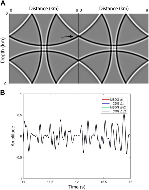
FIGURE 4. (A) Snapshots of the wavefields generated by the MSDG and CDG methods at t = 2 s, where the left part is generated by the MSDG method and the right part is generated by the CDG method. The arrow indicates that there is a slight phase shift. (B) Normalized waveforms within the time interval of [11 s, 13 s].

FIGURE 5

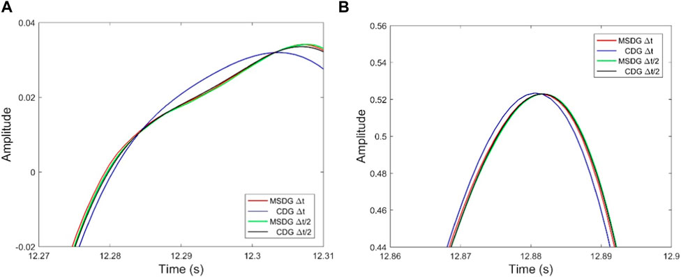
FIGURE 5. Normalized waveforms in time intervals of (A) [12.27 s, 12.31 s] and (B) [12.86 s, 12.90 s], which are clear observations of Figure 4.

4.2 Elastic wave propagation models

Here, the elastic wavefield propagation in two models are considered. The first model is a square domain with $0\le x,z\le 6$ km. The domain is discretized with uniform rectangles with 20 m × 20 m. The density is ρ = 1.8 g/cm³. P and SV wave speeds are c_p = 3.456 km/s and c_s = 2.160 km/s. A point source is set at (3.0 km, 3.0 km) with similar time variation function as in Eq. 21 where f₀ = 20 Hz. We set a receiver at (2.4 km, 3.8 km) to record the synthetic seismogram. The MSDG method with order κ = 2 of the basis function is used for computing. The time increment is ∆t = 1.16 ms.

Figure 6 shows the elastic wavefield snapshot at time 0.85 s, from which we see clear wavefronts without visible numerical dispersion. To observe more clearly, we plot the normalized waveforms at t $\in$ [0 s, 1.4 s] in Figure 7. The solid line is the numerical result generated by the MSDG method, and the dotted line is the reference result generated by the staggered grid method (Virieux, 1986) on fine grids. We see that the two solutions fit well, illustrating the correctness of our method.

FIGURE 6

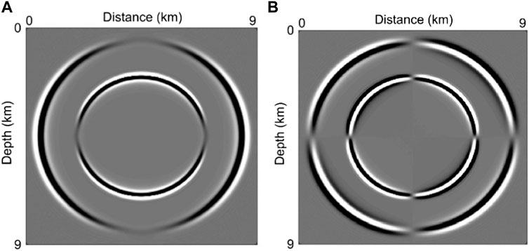
FIGURE 6. Snapshots of the elastic wavefields in homogeneous isotropic medium. (A) u₁ and (B) u₂.

FIGURE 7

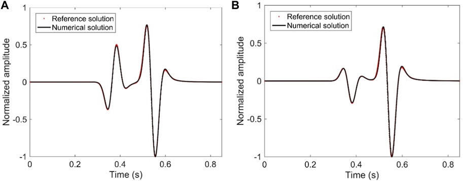
FIGURE 7. Normalized waveform records computed by the MSDG method within the time interval of [0 s, 0.8 s] in homogeneous medium. (A) u₁ and (B) u₂.

The second homogeneous elastic model is the Lamb’s model, in which the long side extends 4 km, and the left boundary has a length of 2 km. The surface is a slope with a tilt angle θ = 10^o. P and SV wave speeds are c_p = 3.2 km/s and c_s = 1.848 km/s, respectively. A point source is located at the upper surface, and its evolution equation is:

$f\left(t\right)=\left(t-t_0\right)\exp \left(-{\left(\pi f_0\left(t-t_0\right)\right)}^2\right),\mathrm{w}\mathrm{i}\mathrm{t}\mathrm{h}\left(f_1,f_2\right)=\left(-\sin \theta ,\cos \theta \right)f\left(t\right)(22)$

where f₀ = 12 Hz, and t₀ is the decay time with t₀ = 0.08 s. We discretize the model with unstructured triangles, and the average length is 30 m with a time step of 0.938 ms.

For the upper surface boundary, we use a free surface boundary condition (FSBC) which says: σ (u)∙n = 0. According to the practice of Rivière (2008), the integral term in Eq. 12 related to this boundary vanishes, so that the FSBC is automatically obtained. Figure 8 shows the elastic wavefield snapshots at t = 0.6 s. The wavefronts are clear without visible numerical dispersion. Particularly, the Rayleigh wave can be clearly observed, demonstrating that the MSDG method is convenient and effective to deal with FSBC.

FIGURE 8

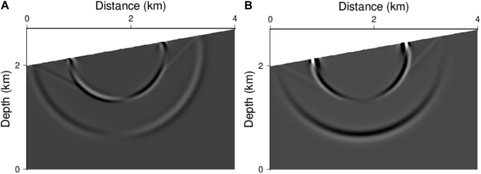
FIGURE 8. Snapshots of the elastic wavefields at t = 0.6 s (A) u₁ and (B) u₂.

4.3 Anisotropic model

This experiment considers a vertical transversely isotropic mode with surface topography (notice that He et al., 2019 used a similar model to study the acoustic wavefields). This model is divided by 66,051 triangles, and the average length is 30 m. A point source with central frequency f₀ = 20 Hz is used with similar time variation function as in Eq. 21, and it is located at (3.6 km, 2.5 km). The material parameters are: ρ = 2.1 g/cm³, c₁₁ = 18.9 GPa, c₁₃ = 8.96 GPa, c₃₃ = 4.725 GPa, and c₄₄ = 28.35 GPa. The time step is 0.3 ms. We use FSBC to deal with topography.

The resulting snapshots at t = 0.35 s and 0.7 s are shown in Figures 9, 10, respectively. The wave fronts are clear. Moreover, the obvious anisotropic propagation of wavefields can be observed. This experiment shows that that the MSDG method is appropriate for wavefield simulations in complicated anisotropic medium.

FIGURE 9

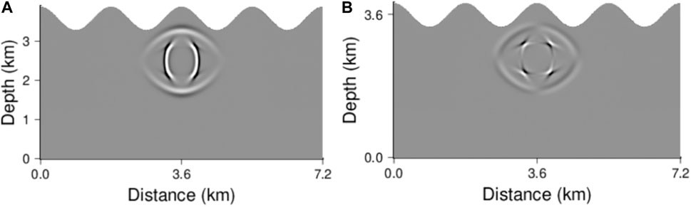
FIGURE 9. Snapshots of the elastic wavefields in anisotropic medium at t = 0.35 s (A) u₁ and (B) u₂.

FIGURE 10

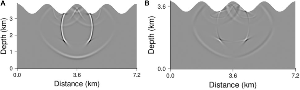
FIGURE 10. Snapshots of the elastic wavefields in anisotropic medium at t = 0.7 s (A) u₁ and (B) u₂.

4.4 Heterogeneous case

The last experiment concentrates on the acoustic wave propagation in 2D SEG/EAGE model. This is a typical heterogeneous model with large speed contrast. The speed structure is shown in Figure 11, the maximum speed of which is 4.482 km/s and the minimum speed is 1.5 km/s. The domain is discretized by regular quadrangular meshes with length of 15 m. The time step is 0.84 ms. The source is located at the center of the domain with similar evolution equation as in Eq. 21 where f₀ = 20 Hz. The MSDG method with order κ = 2 of the basis function is used for simulation. Figure 12 presents the wavefield snapshots at t= 0.35 and 0.7 s. Clear wavefronts are observed, and the reflected, refracted, and scattered waves can be clearly identified. This test demonstrates that the MSDG method is promising for wavefield modeling in complicated heterogeneous medium.

FIGURE 11

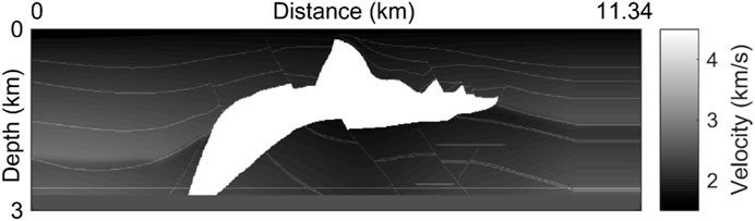
FIGURE 11. Acoustic velocity structure of the SEG/EAGE model.

FIGURE 12

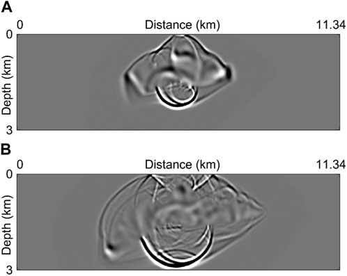
FIGURE 12. Snapshots of the acoustic wavefields at (A) t = 0.35 s and (B) t = 0.7 s.

5 Conclusion

We propose a new MSDG method for 2D seismic wavefield modeling, the temporal discretization of which employs a modified symplectic partitioned Runge–Kutta scheme which has minimized phase error, and the space discretization is based on the symmetric interior penalty Galerkin formulations. The numerical stability condition of the MSDG method is investigated in detail. We compare the stability results with classic SDG and CDG methods, and it is indicated that the proposed method has more relaxed maximum Courant numbers than the other two methods. We study the dispersion and dissipation of the MSDG method, and find that MSDG produces smaller dispersion than SDG and CDG. Moreover, both MSDG and SDG methods are non-dissipative that have beneficial effect on long-term simulations, whereas the CDG method introduces a large numerical dissipation. These conclusions confirm the advantages of symplectic time-stepping method over non-symplectic scheme in keeping energy conservation. Finally, we perform some tests on wave propagation in homogeneous and heterogeneous media. Both isotropic and anisotropic cases are considered. A long time simulation is also carried out. The numerical results show that the MSDG method has good abilities to suppress the numerical dispersion and is suitable for wavefield simulations with regular and irregular geometric areas, especially suitable for long time simulation.

The research presented in this paper is currently applicable to the 2D case. In fact, our method can be directly generalized to 3D case. The program implementation in this study is serial, and the design of parallel computing is imminent. These are the focus of future research.

Data availability statement

The raw data supporting the conclusion of this article will be made available by the authors, without undue reservation.

Author contributions

XHe makes contributions to the code and writing of the original draft; JZ makes contributions to the modeling and writing-editing; JS, XHu, and YZ check all the data and revise the language.

Funding

This work was supported by the Project of Cultivation for Young Top-notch Talents of Beijing Municipal Institutions (Grant No. BPHR202203047), the Young Elite Scientists Sponsorship Program by BAST, and the National Natural Science Foundation of China (Grant Nos. 41974114, 11961020).

Conflict of interest

The authors declare that the research was conducted in the absence of any commercial or financial relationships that could be construed as a potential conflict of interest.

Publisher’s note

All claims expressed in this article are solely those of the authors and do not necessarily represent those of their affiliated organizations, or those of the publisher, the editors and the reviewers. Any product that may be evaluated in this article, or claim that may be made by its manufacturer, is not guaranteed or endorsed by the publisher.

References

Ainsworth, M., Monk, P., and Muniz, W. (2006). Dispersive and dissipative properties of discontinuous Galerkin finite element methods for the second-order wave equation. J. Sci. Comput. 27 (1), 5–40. doi:10.1007/s10915-005-9044-x

CrossRef Full Text | Google Scholar

Chen, J. B. (2009). Lax Wendroff and Nyström methods for seismic modelling. Geophys. Prospect. 57 (6), 931–941. doi:10.1111/j.1365-2478.2009.00802.x

CrossRef Full Text | Google Scholar

Chen, K. H. (1984). Propagating numerical model of elastic wave in anisotropic in homogeneous media-finite element method. 54th SEG Annu. Meet. Expand. Abstr., 631–632.

Google Scholar

Cockburn, B., and Shu, C. W. (2001). Runge–Kutta discontinuous Galerkin methods for convection-dominated problems. J. Sci. Comput. 16 (3), 173–261.

Google Scholar

Dablain, M. A. (1986). The application of high order differencing to the scalar wave equation. Geophysics 51 (1), 54–66. doi:10.1190/1.1442040

CrossRef Full Text | Google Scholar

Dawson, C., Sun, S., and Wheeler, M. F. (2004). Compatible algorithms for coupled flow and transport. Comput. Methods Appl. Mech. Eng. 193 (23-26), 2565–2580. doi:10.1016/j.cma.2003.12.059

CrossRef Full Text | Google Scholar

de Basabe, J. D., and Sen, M. K. (2010). Stability of the high-order finite elements for acoustic or elastic wave propagation with high-order time stepping. Geophys. J. Int. 181 (1), 577–590. doi:10.1111/j.1365-246x.2010.04536.x

CrossRef Full Text | Google Scholar

de Basabe, J. D., Sen, M. K., and Wheeler, M. F. (2008). The interior penalty discontinuous Galerkin method for elastic wave propagation: Grid dispersion. Geophys. J. Int. 175 (1), 83–93. doi:10.1111/j.1365-246x.2008.03915.x

CrossRef Full Text | Google Scholar

de Hoop, A. (1960). A modification of Cagniard’s method for solving seismic pulse problems. Appl. Sci. Res. Sect. B 8 (1), 349–356. doi:10.1007/bf02920068

CrossRef Full Text | Google Scholar

Étienne, V., Chaljub, E., Virieux, J., and Glinsky, N. (2010). An hp-adaptive discontinuous Galerkin finite-element method for 3-D elastic wave modelling. Geophys. J. Int. 183 (2), 941–962. doi:10.1111/j.1365-246x.2010.04764.x

CrossRef Full Text | Google Scholar

Feng, K., and Qin, M. (2010). Symplectic geometric algorithms for Hamiltonian systems, 449. Berlin, Germany: Springer.

Google Scholar

Ferroni, A., Antonietti, P. F., Mazzieri, I., and Quarteroni, A. (2017). Dispersion-dissipation analysis of 3-D continuous and discontinuous spectral element methods for the elastodynamics equation. Geophys. J. Int. 211 (3), 1554–1574. doi:10.1093/gji/ggx384

CrossRef Full Text | Google Scholar

Fornberg, B. (1998). A practical guide to pseudospectral methods (No.1). Cambridge, UK: Cambridge University Press.

Google Scholar

Grote, M. J., Schneebeli, A., and Schötzau, D. (2006). Discontinuous Galerkin finite element method for the wave equation. SIAM J. Numer. Analysis 44 (6), 2408–2431. doi:10.1137/05063194x

CrossRef Full Text | Google Scholar

Hairer, E., Lubich, C., and Wanner, G. (2006). Geometric numerical integration: Structure-preserving algorithms for ordinary differential equations. Berlin, Germany: Springer Science and Business Media.

Google Scholar

He, X. J., Li, J. S., Huang, X. Y., and Zhou, Y. J. (2022a). Solving elastic wave equations in 2D transversely isotropic media by a weighted Runge-Kutta discontinuous Galerkin method. Petroleum Sci. doi:10.1016/j.petsci.2022.10.007

CrossRef Full Text | Google Scholar

He, X., Yang, D., Huang, X., and Ma, X. (2020a). A numerical dispersion-dissipation analysis of discontinuous Galerkin methods based on quadrilateral and triangular elements. Geophysics 85 (3), T101–T121. doi:10.1190/geo2019-0109.1

CrossRef Full Text | Google Scholar

He, X., Yang, D., Ma, X., and Qiu, C. (2020b). A modified numerical-flux-based discontinuous Galerkin method for 2D wave propagations in isotropic and anisotropic media. Geophysics 85 (5), T257–T273. doi:10.1190/geo2019-0485.1

CrossRef Full Text | Google Scholar

He, X., Yang, D., Ma, X., and Zhou, Y. (2019). Symplectic interior penalty discontinuous Galerkin method for solving the seismic scalar wave equation. Geophysics 84 (3), T133–T145. doi:10.1190/geo2018-0492.1

CrossRef Full Text | Google Scholar

He, X., Yang, D., Qiu, C., Zhou, Y., and Ma, X. (2022b). An efficient discontinuous Galerkin method using a tetrahedral mesh for 3D seismic wave modeling. Bull. Seismol. Soc. Am. 112 (3), 1197–1223. doi:10.1785/0120210229

CrossRef Full Text | Google Scholar

Igel, H. (2017). Computational seismology: A practical introduction. Oxford, UK: Oxford University Press.

Google Scholar

Iwatsu, R. (2009). Two new solutions to the third-order symplectic integration method. Phys. Lett. A 373 (34), 3056–3060. doi:10.1016/j.physleta.2009.06.048

CrossRef Full Text | Google Scholar

Käser, M., and Dumbser, M. (2006). An arbitrary high-order discontinuous Galerkin method for elastic waves on unstructured meshes-I: The two-dimensional isotropic case with external source terms. Geophys. J. Int. 166 (2), 855–877. doi:10.1111/j.1365-246x.2006.03051.x

CrossRef Full Text | Google Scholar

Komatitsch, D., and Vilotte, J. P. (1998). The spectral element method: An efficient tool to simulate the seismic response of 2D and 3D geological structures. Bull. Seism. Soc. Am. 88 (2), 368–392. doi:10.1785/bssa0880020368

CrossRef Full Text | Google Scholar

Kosloff, D. D., and Baysal, E. (1982). Forward modeling by a Fourier method. Geophysics 47 (10), 1402–1412. doi:10.1190/1.1441288

CrossRef Full Text | Google Scholar

Li, B. Q. (2006). Discontinuous Finite Elements in Fluid Dynamics and Heat Transfer, 578. Berlin, Germany: Springer Science & Business Media.

Google Scholar

Liu, S. L., Yang, D. H., Lang, C., Wang, W., and Pan, Z. (2017). Modified symplectic schemes with nearly-analytic discrete operators for acoustic wave simulations. Comput. Phys. Commun. 213, 52–63. doi:10.1016/j.cpc.2016.12.002

CrossRef Full Text | Google Scholar

Liu, S., Yang, D., Dong, X., Liu, Q., and Zheng, Y. (2017). Element-by-element parallel spectral-element methods for 3-D teleseismic wave modeling. Solid earth 8 (5), 969–986. doi:10.5194/se-8-969-2017

CrossRef Full Text | Google Scholar

Liu, Y., and Sen, M. K. (2009). An implicit staggered-grid finite-difference method for seismic modelling. Geophys. J. Int. 179 (1), 459–474. doi:10.1111/j.1365-246x.2009.04305.x

CrossRef Full Text | Google Scholar

Ma, X., and Yang, D. H. (2017). A phase-preserving and low-dispersive symplectic partitioned Runge-Kutta method for solving seismic wave equations. Geophys. J. Int. 209 (3), 1534–1557. doi:10.1093/gji/ggx097

CrossRef Full Text | Google Scholar

Ma, X., Yang, D. H., and Liu, F. Q. (2011). A nearly analytic symplectically partitioned Runge-Kutta method for 2-D seismic wave equations. Geophys. J. Int. 187 (1), 480–496. doi:10.1111/j.1365-246x.2011.05158.x

CrossRef Full Text | Google Scholar

Meng, W., and Fu, L. Y. (2018). Numerical dispersion analysis of discontinuous Galerkin method with different basis functions for acoustic and elastic wave equations. Geophysics 83 (3), T87–T101. doi:10.1190/geo2017-0485.1

CrossRef Full Text | Google Scholar

Meng, W., and Fu, L. Y. (2017). Seismic wavefield simulation by a modified finite element method with a perfectly matched layer absorbing boundary. J. Geophys. Eng. 14 (4), 852–864. doi:10.1088/1742-2140/aa6b31

CrossRef Full Text | Google Scholar

Rivière, B. (2008). Discontinuous Galerkin methods for solving elliptic and parabolic equations: Theory and implementation. Philadelphia, PA,USA: Society for Industrial and Applied Mathematics.

Google Scholar

Rivière, B., and Wheeler, M. F. (2003). Discontinuous finite element methods for acoustic and elastic wave problems. Contemp. Math. 329 (271-282), 4–6.

Google Scholar

Sei, A., and Symes, W. (1995). Dispersion analysis of numerical wave propagation and its computational consequences. J. Sci. Comput. 10 (1), 1–27. doi:10.1007/bf02087959

CrossRef Full Text | Google Scholar

Tarantola, A. (1984). Inversion of seismic reflection data in the acoustic approximationflection data in the acoustic approximation. Geophysics 49, 1259–1266. doi:10.1190/1.1441754

CrossRef Full Text | Google Scholar

Tong, P., Komatitsch, D., Tseng, T. L., Hung, S. H., Chen, C. W., Basini, P., et al. (2014). A 3 D spectral element and frequency wave number hybrid method for high resolution seismic array imaging. Geophys. Res. Lett. 41 (20), 7025–7034. doi:10.1002/2014gl061644

CrossRef Full Text | Google Scholar

Virieux, J. (1986). P-SV wave propagation in heterogeneous media: Velocity-stress finite-difference method. Geophysics 51 (4), 889–901. doi:10.1190/1.1442147

CrossRef Full Text | Google Scholar

Wilcox, L. C., Stadler, G., Burstedde, C., and Ghattas, O. (2010). A high-order discontinuous Galerkin method for wave propagation through coupled elastic–acoustic media. J. Comput. Phys. 229 (24), 9373–9396. doi:10.1016/j.jcp.2010.09.008

CrossRef Full Text | Google Scholar

Williamson, J. H. (1980). Low-storage Runge-Kutta schemes. J. Comput. Phys. 35 (1), 48–56. doi:10.1016/0021-9991(80)90033-9

CrossRef Full Text | Google Scholar

Yang, D. H. (2002). Finite element method of the elastic wave equation and wavefield simulation in two-phase anisotropic media. Chin. J. Geophys. 45 (4), 575–583.

CrossRef Full Text | Google Scholar

Yang, D. H., He, X. J., Ma, X., Zhou, Y. J., and Li, J. (2016). An optimal nearly analytic discrete-weighted Runge-Kutta discontinuous Galerkin hybrid method for acoustic wavefield modeling. Geophysics 81 (5), T251–T263. doi:10.1190/geo2015-0686.1

CrossRef Full Text | Google Scholar

Yang, D., Song, G., Chen, S., and Hou, B. (2007). An improved nearly analytical discrete method: An efficient tool to simulate the seismic response of 2-D porous structures. J. Geophys. Eng. 4 (1), 40–52. doi:10.1088/1742-2132/4/1/006

CrossRef Full Text | Google Scholar

Yang, D., Teng, J., Zhang, Z., and Liu, E. (2003). A nearly analytic discrete method for acoustic and elastic wave equations in anisotropic media. Bull. Seismol. Soc. Am. 93 (2), 882–890. doi:10.1785/0120020125

CrossRef Full Text | Google Scholar

Yang, D., Tong, P., and Deng, X. (2012). A central difference method with low numerical dispersion for solving the scalar wave equation. Geophys. Prospect. 60 (5), 885–905. doi:10.1111/j.1365-2478.2011.01033.x

CrossRef Full Text | Google Scholar