Papua New Guinea Moho inversion based on XGM 2019e gravity field model

The construction of the high-resolution Moho depth model is significant for studying the characteristics of the complex tectonic movement (seafloor spreading, plate subduction phenomena) in Papua New Guinea. We calculate the region’s Moho relief and lithosphere thinning factor using the XGM 2019e gravity field model and nonlinear fast gravity inversion method under the GEMMA Moho depth model’s constraint considering the influence of lithosphere thermal gravity anomaly. The calculation result shows that the Moho depth is between 6—34 km, forming two large depressions in Woodlark Basin (WB) and Solomon Sea Plate (SSP) with deep scattered islands. In addition, the findings suggest that Significant differences exist in the shape and tectonic movement intensity of the North and South oceanic crust at the WB. Nevertheless, the lithosphere extends evenly in Manus Basin (MB). WB collided with the Solomon Islands at a higher angle than the SSP subducted under Bismarck Sea Plate (BSP); strong earthquakes may frequently occur on both sides and in deeper positions at West New Britain Trench in the future.

1 Introduction

Papua New Guinea is in the northeast of Australia and southwest of the Pacific Ocean, situated at the junction of the Pacific Plate and the Indo-Australian plate, composed of several microplates (Wallace et al., 2004; Davies, 2012) (Figure 1). The region has undergone a series of tectonic movements such as plate subduction, arc-continent collision, and seafloor spreading (Curtis, 1973), which indirectly or directly led to strong earthquakes and tsunamis (Borrero et al., 2003; Xu et al., 2020). Since the Cretaceous, the convergence and subduction of the Indo-Australian and Pacific plate caused the rise of seafloor sediments, which in turn rose to form arcs and collided with the Australian continent (Pigram and Davies, 1987; Haddad and Watts, 1999). There are still intricate motions between multiple microplates or accretion blocks. For instance, WB subducted into the Solomon Islands; SSP subducted beneath BSP; BSP moved southwest due to the Finisterre collision (Wallace et al., 2004); Finisterre, Adelbert block ran into Guinea Plateau. The interaction between microplates leads to strong plate coupling (Mann et al., 1998), which results in regional uplift and folds (Curtis, 1973). The phenomenon of seafloor spreading primarily occurs in three areas, namely, WB, MB, and SSP, with varying intensities, periods, and forms. The spreading center of WB moves from east to west at a quick speed of 14 cm/yr from 3.6 Ma and continuously goes through the spreading center nucleation, expansion, and standstill (Taylor et al., 1999). In the young (<1 Ma) back-arc MB (Dyriw et al., 2021), Martinez and Taylor (1996) found that the spreading center diffuses outward at a rate of 9.2 cm/yr to form a wedge-shaped oceanic crust. The SSP spread at a relatively slow rate of 5.8 cm/yr for a long time (Joshima et al., 1987), which is partially subducted below the BSP and Trobriand Trench (Honza et al., 1987).

FIGURE 1

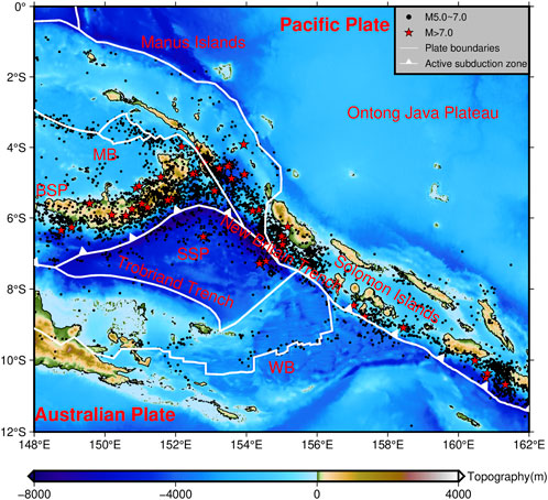
FIGURE 1. Topography and earthquake occurrence in Papua New Guinea. The earthquake data comes from United States Geological Survey (USGS) (e.g., earthquakes with a magnitude greater than 5.0 since 1980 are considered); topography data are obtained from General Bathymetric Chart of the Oceans 2021 (GEBCO 2021); plate boundary data is taken from Bird. (2003).

Previous research has investigated variable tectonic movements from various perspectives. Nonetheless, our understanding of the overall deep structure characteristics remains limited due to a few previous research on this aspect, and the existing Moho depth models have low resolution (up to 0.5°×0.5°). The Moho relief and lithosphere thinning factor are critical parameters that present deep structure features: the former describes the overall crustal structure (Zhu, 2000) and is closely linked to tectonic evolution, such as plate subduction; the latter indicates the degree of thinning of the lithosphere, which can measure the extent and intensity of seafloor spreading. Solving both data with higher resolution can help us better understand the details and characteristics of the deep structure of the region.

In recent studies, the Moho relief has been determined through five different methods: seismic refraction, receiver functions, seismic reflection profiles, seismic tomography, and gravity inversion (Aitken et al., 2013). While several seismic techniques provide relatively accurate Moho depth results, they are limited to individual points, sections, or strip areas. They are not suitable for large-scale research due to high costs. As a result, using gravity data has become a more popular alternative approach in geophysics due to its high resolution, extensive coverage, and richer sources. Nonetheless, some hyperparameters must be selected during the gravity inversion, such as Moho reference depth (the depth of the normal Earth) and crust-mantle density contrast. To enhance the accuracy of Moho depth inversion results, many researchers use seismic data as constraint information to determine hyperparameters by minimizing the misfit between the gravimetric solution and the seismic data. For example, Gaulier et al. (1997) determined the Moho reference depth and crust-mantle density contrast of the Liguro-Provençal Basin’s Moho depth based on seismic refraction and reflection data. The Moho depth obtained by the seismic method was broadly consistent with the gravity inversion result, with a difference of less than 2 km; Aitken. (2010) also inverted the Australian Moho depth using various interface models and seismic data constraints, revealing that seismically-constrained gravity inversion can generate a well-constrained and detailed Moho depth model (Abrehdary et al., 2015).

Gravity corrections are crucial for improving the accuracy of Moho depth inversion results. In addition to topography and other common corrections, lithosphere thermal gravity anomaly correction is essential in Papua New Guinea. Seafloor spreading results in the extension and thinning of the oceanic lithosphere and adjacent rifted continental margin lithosphere, resulting in the geothermal rise and lithosphere lateral density change (Chappell and Kusznir, 2008), which generates significant lithosphere thermal gravity anomaly, reaching the maximum at the ocean ridge (Alvey et al., 2008). Chappell and Kusznir. (2008) obtained lithosphere thermal gravity anomaly through iterative calculation combined with the lithosphere thinning temperature field model proposed by McKenzie. (1978). He considered the existence of the crustal melting thickness (White and McKenzie, 1989) and evaluated the sensitivity of the thermal model. Alvey et al. (2008) established multiple plate reconstruction models to estimate the age of the oceanic lithosphere, providing more methods for calculating lithosphere thermal gravity anomaly. After correcting the lithosphere thermal gravity anomaly, the inversion result will be more accurate and closer to the actual geological structure (Cowie and Kusznir, 2012; Constantino and Sacek, 2020).

Based on the reasons mentioned above, we propose to use the Moho depth of the GEMMA model as constraint information, along with Bouguer gravity anomaly data (After lithosphere thermal gravity anomaly correction) to obtain the Moho depth and distribution of lithosphere thinning factors in Papua New Guinea through gravity inversion, focusing on the Moho relief, seafloor spreading and microplate subduction. The paper is structured as follows: 1) Data source: presentation of the Bouguer gravity anomaly data required for gravity inversion, the GEMMA Moho depth data, and the relevant data for calculating the lithosphere thermal gravity anomaly. 2) Methodology: presentation of the gravity inversion and lithosphere thermal gravity anomaly calculation methods. 3) Results and discussion: description and analysis of the Moho inversion results, lithosphere thermal gravity anomaly, lithosphere thinning factor results, the seafloor spreading features at WB and MB, and microplate subduction at SSP and WB. 4) Conclusion: summary of the work carried out.

2 Data source

We use the combined global gravity field model XGM 2019e (Zingerle et al., 2020) as the raw gravity data. This model integrates terrestrial and satellite altimetry data based on the spherical harmonic domain. Its spherical harmonic is 2’ (the spatial resolution is about 4 km). According to the GNSS/levelling validation test and Ocean Mean Dynamic Topography (MDT) calculation results, XGM 2019e′s performance is more consistent globally than preceding models, especially in the ocean.

For the terrain correction, we use the spherical approximation classical gravity anomaly obtained from the model minus the attraction of the Bouguer plate, in which the topography spherical harmonic model of ETOPO1 data (Amante and Eakins, 2009) up to the same maximum degree is used (Standard density of 2,670 $\mathrm{k}\mathrm{g}/{\mathrm{m}}^3$ for the continents, −1,025 $\mathrm{k}\mathrm{g}/{\mathrm{m}}^3$ for the oceans), then resample the calculations into Bouguer gravity anomaly data with a spatial resolution of 3′for gravity inversion. The overall variation range is about −200–400 mGal, showing apparent high anomaly in several oceanic basins and low anomaly in densely distributed islands (Figure 2A). There are two major gravity anomaly gradient zones with drastic variation, located at the junction of plate subduction, which are the areas where earthquakes occur frequently. They are the SE-NW trend of SSP-MB and the SW-NE trend of WB - Solomon Islands-Ontong Java Plateau.

FIGURE 2

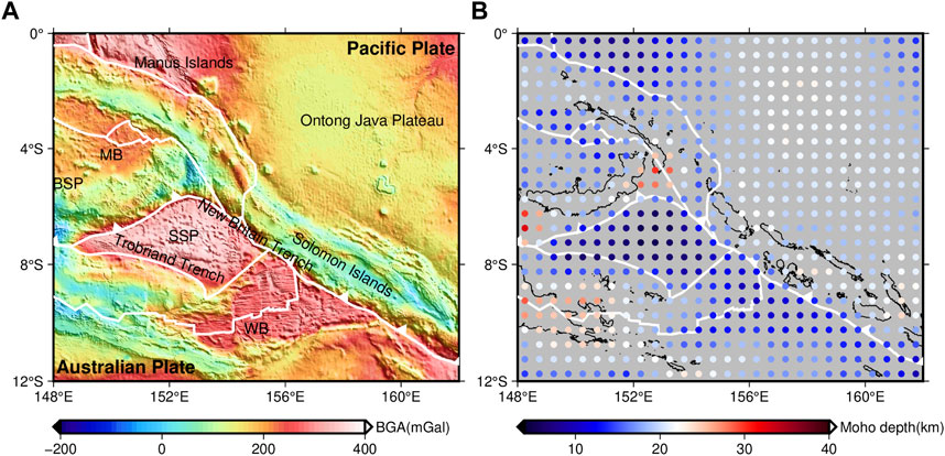
FIGURE 2. (A) The calculated Bouguer gravity anomaly, (B) Moho depth of GEMMA model.

In the study area, only a few Moho depth point data values obtained by the seismic method exists at WB and Manus Islands, so we can’t understand the characteristics of Moho relief as a whole. We only use this data to verify our Moho depth inversion result. Therefore, this paper intends to use the Moho depth (with respect to sea level) provided by the GEMMA Earth crust model (Reguzzoni and Sampietro, 2015) as the depth constraint information. The spatial resolution of the model is $0.5°\times 0.5°$, and the Moho depth error standard deviation is 3.4 km globally. It is calculated using a uniformly distributed GOCE gravity satellite dataset and CRUST2.0 seismic information through least squares inversion, considering many factors, such as differences between major geological provinces and lateral density variations of the upper mantle. The model’s gravitational effects are more consistent with the actual gravity field, so it can be used as a reference for studying Moho relief in some places lacking seismic data. We select 1760 Moho depth points from the model, as shown in Figure 2B. Model’s Moho depth is between 5∼40 km. Along the SW-NE direction, the depth decreases slowly, then increases sharply, and finally decreases gradually. The minimum depth is found at the SSP and WB, while the maximum depth is at the Solomon Islands and locations close to the Ontong Java Plateau.

Lithosphere thermal equilibration time (Figure 3) are needed to calculate the lithosphere thermal gravity anomaly. In oceanic lithosphere, the lithosphere thermal equilibration time is the age of oceanic crust, which is taken from Müller et al. (2019). In continental margin lithosphere, the lithosphere thermal equilibration time is the age since continental breakup, we set it as 32 Ma (Wu et al., 2017).

FIGURE 3

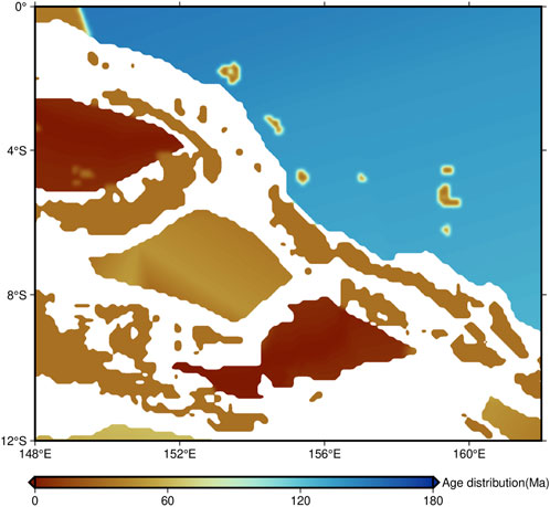
FIGURE 3. Distribution of lithosphere thermal equilibration time in Papua New Guinea.

3 Methodology

3.1 Gravity inversion

The fast nonlinear gravity inversion based on spatial spherical coordinate proposed by Uieda and Barbosa. (2017) is adopted to study the Moho depth’s solution. This approach considers the influence of Earth curvature on the calculation result (Uieda et al., 2015). Moreover, it enhances the inversion calculation efficiency by using Silva et al. (2014) of replacing Jacobian matrix with a Bouguer plate.

To reduce the ill-posed solution of the inversion problem, regularization constraint is introduced to make the inversion result smoother and closer to the real situation (Silva et al., 2001). The inversion objective function $\mathrm{\Gamma }\left(\mathit{P}\right)$ constructed according to the gravity data fitting term and regularization term is as follows:

$\mathrm{\Gamma }\left(\mathit{P}\right)={\left[{\mathit{d}}^0-\mathit{d}\left(\mathit{p}\right)\right]}^T\left[{\mathit{d}}^0-\mathit{d}\left(\mathit{p}\right)\right]+\mu {\mathit{p}}^T{\mathbf{R}}^{\mathrm{T}}\mathbf{R}\mathit{p}(1)$

Where $\mathit{p}$ represents the Moho depth parameter vector, $\mathit{d}\left(\mathit{p}\right)$ is the gravity anomaly prediction data vector calculated by $\mathit{p}$, ${\mathit{d}}^0$ is the gravity anomaly observation data vector, $\mathbf{R}$ is the first-order difference matrix representing the depth of adjacent spherical prisms, and $\mu$ is the regularization parameter.

The Gauss-Newton iteration method minimizes the objective function. The perturbation vector $∆\mathit{p}$ updates the parameter vector $\mathit{p}$ through the iteration process until the objective function reaches the optimal solution. At the k+1st iteration, the parameter vector ${\mathit{p}}^{k+1}$ is updated as follows:

${\mathit{p}}^{k+1}={\mathit{p}}^k+∆{\mathit{p}}^k(2)$

The perturbation vector of the kth iteration is obtained by solving linear Eq. (3):

$\left[{\mathbf{A}}^{{\mathrm{k}}^{\mathrm{T}}}{\mathbf{A}}^{\mathrm{k}}+\mu {\mathbf{R}}^{\mathrm{T}}\mathbf{R}\right]∆{\mathit{p}}^k={\mathbf{A}}^{{\mathrm{k}}^{\mathrm{T}}}\left[{\mathit{d}}^0-\mathit{d}\left({\mathit{p}}^k\right)\right]-\mu {\mathbf{R}}^{\mathrm{T}}\mathbf{R}{\mathit{p}}^k(3)$

$\mathbf{A}=2\mathrm{\pi }\mathrm{G}∆\rho \mathbf{I}(4)$

In which G is the gravitational constant, $∆\rho$ is the crust-mantle density contrast, and $\mathbf{I}$ is the identity matrix.

We determine the three hyperparameters needed for the inversion by two cross-validations: The Moho reference depth ($z^{ref}$), crust-mantle density contrast ($∆\rho$), and regularization parameters ($\mu$). The specific process is as follows:

(1) Divide the Bouguer gravity anomaly data into two data sets: test set and training set. The grid spacing of the training set is twice that of the test set. We apply the training set to invert the Moho depth given three different parameters, while the test set data is used to determine the values of hyperparameters;

(2) Perform the first cross-validation to determine $\mu$. We set the value range and interval of three hyperparameters, choose one $z^{ref}$ and $∆\mathrm{\rho }$ randomly and calculate the mean square error (MSE) between the gravity anomaly obtained by forward calculation of Moho depth obtained by inversion and the test set when different $\mathrm{\mu }$ is selected. The $\mathrm{\mu }$ corresponding to the minimum MSE is taken as the final $\mu$;

(3) Perform the second cross-validation to determine $z^{ref}$ and $∆\rho$. Calculating the MSE between the Moho depth obtained by inversion and the constraint information while selecting different combinations of $z^{ref}$ and $∆\rho$. The $z^{ref}$, $∆\rho$ correspond to the minimum MSE that is taken as the optimal solution.

3.2 Lithosphere thermal gravity anomaly correction

To calculate lithosphere thermal gravity anomaly, we first need to estimate temperature anomaly at different depths in the lithosphere. We divide the study region into 141×121 grids with a vertical spacing of 5 km and utilize the lithosphere thinning temperature field model (McKenzie, 1978) to calculate the temperature anomaly caused by lithosphere stretching based on the assumption that the stretching degree of the lithosphere is equal to the crust. The temperature anomaly in °C, $T_z$, at depth $z$ is:

$\begin{array}{c}{T}_z=\frac{2{\mathrm{T}}_{\mathrm{m}}}{\mathrm{\pi }}{\displaystyle \sum _{n=0}^{\infty }}\frac{{\left(-1\right)}^{n+1}}{n}\left[\frac{\beta }{n\mathrm{\pi }}\sin \left(\frac{n\mathrm{\pi }}{\beta }\right)\times \exp \left(-\frac{n^{2}t}{\mathrm{\tau }}\right)\sin \left(\frac{n\mathrm{\pi }z}{\mathrm{a}}\right)\right]\end{array}(5)$

where the base-lithosphere temperature ${\mathrm{T}}_{\mathrm{m}}$ = 1,300°C, lithosphere cooling thermal decay constant $\mathrm{\tau }$ = 65 Ma, and the equilibrium lithosphere thickness $\mathrm{a}$ = 125 km (Greenhalgh and Kusznir, 2007). The description of lithosphere thermal equilibration time $t$ is provided in the Data Source section.

The selection of lithosphere stretching factor $\beta$ can be divided into two cases. For oceanic lithosphere, $\beta =\infty$. For continental margin lithosphere, the original crustal thickness $\mathrm{C}{\mathrm{t}}_{\mathrm{i}\mathrm{n}\mathrm{i}\mathrm{t}}$ is set as 32 km (Wu et al., 2017), and $\beta$ is equal to the ratio of the original crustal thickness $\mathrm{C}{\mathrm{t}}_{\mathrm{i}\mathrm{n}\mathrm{i}\mathrm{t}}$ to the current crustal thickness $C{t}_{now}$ derived from gravity inversion. At the rifted continental margin, decompression melting makes the crust thick until the seafloor spreads to form a new oceanic crust. Therefore, thickness of magmatic should be considered and $\beta$ is calculated as follows:

$\begin{array}{c}\beta =\frac{\mathrm{C}{\mathrm{t}}_{\mathrm{i}\mathrm{n}\mathrm{i}\mathrm{t}}}{C{t}_{now}-C{t}_{mag}}\end{array}(6)$

where $C{t}_{mag}$ is the thickness of magmatic. We use the relationship between the thinning factor and thickness of magmatic (White and McKenzie, 1989) to calculate $\beta$, set the critical thinning factor $\left(1-1/{\mathrm{\beta }}_{\mathrm{c}\mathrm{r}\mathrm{i}\mathrm{t}}\right)$ = 0.5 and the maximum oceanic crust thickness $\mathrm{C}{\mathrm{t}}_{\max }$ =10 km (Greenhalgh and Kusznir, 2007) (Figure 4). When the lithosphere thinning factor $\left(1-1/\beta \right)$ is less than 0.5, $C{t}_{mag}$ = 0. On the contrary, the influence of magma on crustal stretching needs to be considered.

FIGURE 4

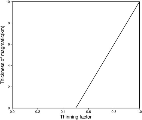
FIGURE 4. Predicted thickness of magmatic as a function of thinning factor.

When the temperature anomaly is calculated, the second step is to calculate the density anomaly. The transition relationship between temperature anomaly and density anomaly is given by:

$∆\rho =-\mathrm{\alpha }\mathrm{\rho }∆T(7)$

in which thermal expansion coefficient $\mathrm{\alpha }$ = $3.28\times {10}^{-5}{\mathrm{K}}^{-1}$, and $\mathrm{\rho }$ = $3300\mathrm{k}\mathrm{g}/{\mathrm{m}}^3$ (Greenhalgh and Kusznir, 2007).

We set each horizontal layer of the grid represents a 5 km thick layer and calculate the lithosphere thermal gravity anomaly of each layer in spherical coordinate. Therefore, the total lithosphere thermal gravity anomaly is the sum of the anomaly calculated for each layer.

3.3 Calculation process

The final Moho relief is obtained by the following steps (Figure 5):

(1) Obtain the initial Moho relief. The Bouguer gravity anomaly data without lithosphere thermal gravity anomaly correction is used for inversion;

(2) Calculate lithosphere thermal gravity anomaly. The crustal thickness is further calculated from the Moho depth obtained in the previous step, and lithosphere thermal anomaly is computed according to the method described above;

(3) Obtain the final Moho relief. The final Moho depth is got through inversion using the Bouguer gravity anomaly data with lithosphere thermal gravity anomaly correction.

FIGURE 5

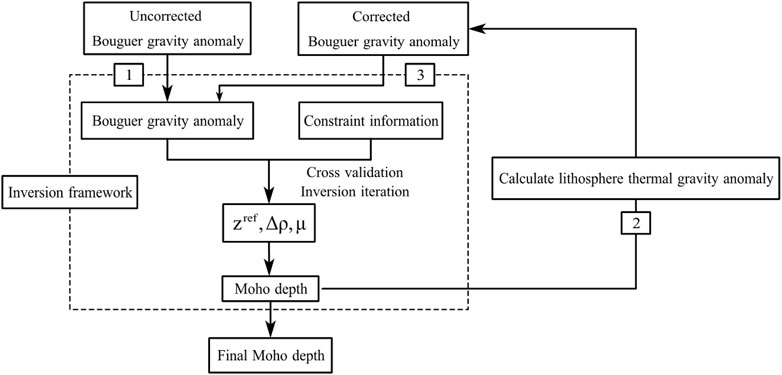
FIGURE 5. Iterative calculation flow chart.

4 Results and discussion

4.1 Moho depth inversion results

The spatial resolution of Moho depth inversion results is 0.1 $°\times$ 0.1 $°$ and the relevant information on the hyperparameters’ selection is shown in Tables 1, 2; Figure 6.

TABLE 1

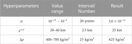
TABLE 1. Hyperparameters’ selection before lithosphere thermal gravity anomaly correction, where $z^{ref}$ is Moho reference depth, $∆\rho$ is crust-mantle density contrast, and $\mu$ is regularization parameters.

TABLE 2

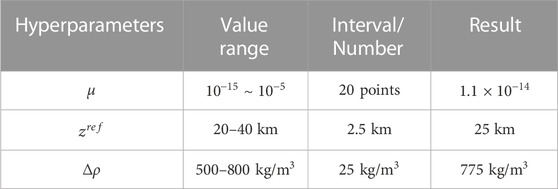
TABLE 2. Hyperparameters’ selection after lithosphere thermal gravity anomaly correction, where $z^{ref}$ is Moho reference depth, $∆\rho$ is crust-mantle density contrast, and $\mu$ is regularization parameters.

FIGURE 6

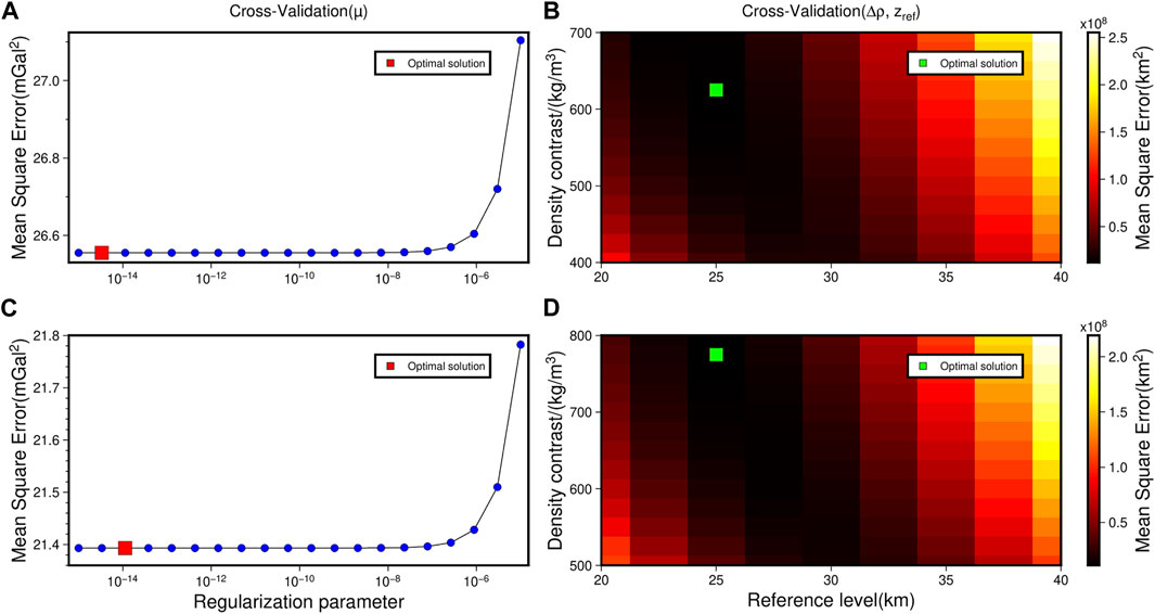
FIGURE 6. Visualization of hyperparameters’ selection. (A, B) are the hyperparameters selection for gravity inversion without lithosphere thermal gravity anomaly correction; (C, D) are the hyperparameters selection for gravity inversion with lithosphere thermal gravity anomaly correction.

The final inversion result after lithosphere thermal gravity anomaly correction (Figure 7B) shows that the Moho relief is consistent with the geological structure and Bouguer gravity anomaly distribution. The Moho depth ranges from 6 to 34 km. The Moho depth at SSP is the lowest (6–8 km), WB is about 10–15 km, and they form two large depressions. Fragmented islands’ Moho is deep, up to 28–34 km. The Moho relief fluctuates gently at Ontong Java Plateau (17–19 km) and MB (12–14 km). There are two depth gradient zones with drastic changes along the strike of SSP-MB and WB-Solomon Islands-Ontong Java Plateau.

FIGURE 7

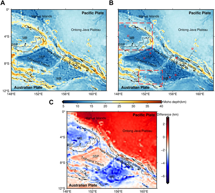
FIGURE 7. Moho depth inversion results. (A) Result without lithosphere thermal gravity anomaly correction, (B) result with lithosphere thermal gravity anomaly correction. The black dotted line is the section profiles. The red dashed rectangular selection range is the area to be studied below. (C) Depth difference between the inversion results after lithosphere thermal gravity anomaly correction and uncorrected inversion results.

Compared to the inversion results without lithosphere thermal gravity anomaly correction (Figures 7A,C), the final inversion result is overall 2–6 km shallower than before. The Moho depth is significantly reduced at locations with young oceanic crust, such as WB (4–6 km), MB (3–5 km), and SSP (1–2 km), which are currently active parts of seafloor spreading, with significant geothermal upwelling and large lateral density variations. This produces large lithosphere thermal gravity anomaly, resulting in great changes in depth after correction. In contrast, Ontong Java Plateau’s Moho depth decreases only by 1–2 km in a wide range, where the oceanic crust is old, and there is no active seafloor spreading, therefore no significant changes in depth after correction.

The misfit analysis all presents normal distribution (Figures 8C, 9C). The residuals between the gravity anomaly obtained by the inversion result’s forward calculation and the gravity anomaly observation have a mean of 0.047 mGal and a Standard deviation (Std) of 6.59 mGal (Figure 8C). The mean depth difference between the inversion result and the GEMMA equals −0.3 km, and Std equals 3.45 km (Figure 8D). After correction, gravity residuals’ mean value of 0.04 mGal and standard deviation of 6.29 mGal (Figure 9C); the depth differences’ mean is 0.18 km, and the standard deviation is 3.31 km (Figure 9D), both of which are reduced from the previous values, indicating that the lithosphere thermal gravity anomaly correction has a positive impact on improving the accuracy of the inversion results.

FIGURE 8

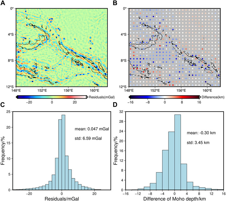
FIGURE 8. The misfit analysis of Moho depth inversion result without lithosphere thermal gravity anomaly correction. (A) The residuals between the gravity anomaly obtained by the inversion result’s forward calculation and the gravity anomaly observation, (B) the Moho depth differences between the inversion result and the GEMMA, (C) histogram of the gravity residuals, and (D) histogram of the Moho depth differences.

FIGURE 9

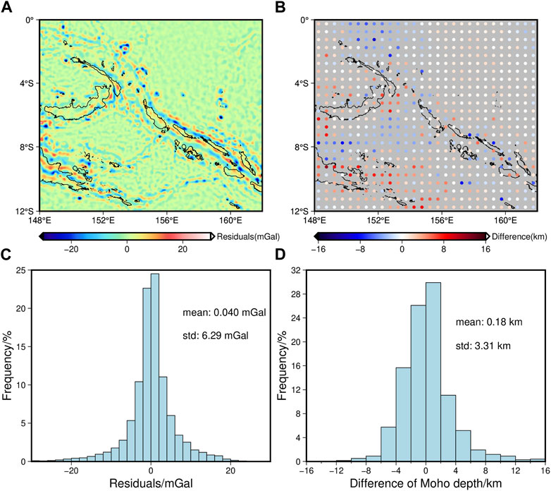
FIGURE 9. The misfit analysis of Moho depth inversion result with lithosphere thermal gravity anomaly correction. The introduction of (A–C), and (D) is the same as that of the corresponding pictures in Figure 8.

The depth difference between the final inversion result and the GEMMA model is smaller in SSP and Ontong Java Plateau than without lithosphere thermal gravity anomaly correction (Figures 8B, 9B), which is because these areas no longer experience active seafloor spreading movements, and the lithosphere thermal gravity anomaly can be more accurately calculated, so these areas’ Moho depth can better be fitted with the GEMMA model after minor correction. In contrast, the Moho depth in the final inversion result is smaller than in the GEMMA model at the southwest corner of MB and WB (Figure 9B). This difference may arise due to the omission of the lithosphere thermal gravity anomaly in the GEMMA model calculation, or it could be attributed to the present-day active seafloor spreading motion, which leads to errors in the gravity anomaly and oceanic crust age data, resulting in inaccuracy in the calculation of the lithosphere thermal gravity anomaly and overcorrection.

Gravity residuals are mainly distributed in the trenches (Figures 8A, 9A), and the maximum Moho depth difference is also primarily located there (Figures 8B, 9B), reaching 8–16 km. This result could be attributed to the fact that trenches are formed by the collision between oceanic and continental plates and are situated at the transition zone between oceanic and continental crust, with a complex geological structure. As a result, gravity anomaly data may be inaccurate and lead to significant discrepancies in Moho depth calculations.

4.2 Lithosphere thinning factor and thermal gravity anomaly calculation results

Figure 10A presents the calculated lithosphere thinning factor (LTF), which shows the highest values at SSP and Manus Islands, at around 1.0, followed by WB, with values ranging from 0.7 to 0.9. The values at MB are slightly larger than that at Ontong Java Plateau (0.3–0.4) by 0.1–0.2. The values at fragmented islands range from 0 to 0.3. Additionally, Figure 10B shows that the lithosphere thermal gravity anomaly (LTGA) is inversely proportional to the age of the oceanic crust, with the largest at WB (−200∼−160 mGal), followed by MB (−160∼ −110 mGal). The values at the SSP range from −137 mGal to −110 mGal. Other areas, such as the Manus Islands and Solomon Islands, are usually between −100 and −70 mGal. In contrast, the values at Ontong Java Plateau are only −20∼−60 mGal.

FIGURE 10

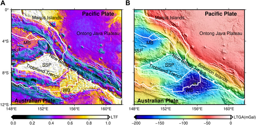
FIGURE 10. Distribution of lithosphere thinning factor and lithosphere thermal gravity anomaly in Papua New Guinea. (A) Lithosphere thinning factor (LTF), (B) lithosphere thermal gravity anomaly (LTGA).

The lithosphere thinning factor and lithosphere thermal gravity anomaly exhibit significant differences between WB and SSP. The SSP continued to spread over the following 10 Ma due to the development of the Solomon rift in the early Oligocene, reaching its peak in the late Oligocene (Honza et al., 1987). Consequently, it underwent prolonged lithosphere stretching and experienced a high degree of thinning. In contrast, WB has a much faster seafloor spreading rate, higher temperature anomaly, and thicker crustal thickness (Figure 13A) than the SSP. The generation of the thin oceanic crust may be due to colder asthenosphere temperature and very slow seafloor spreading rate (Greenhalgh and Kusznir, 2007). Therefore, we speculate that WB has a higher asthenosphere temperature and more intense seafloor spreading activity than the SSP. These factors may explain why the thinning factor at the SSP is higher than that in WB, but the lithosphere thermal gravity anomaly is lower at the SSP.

The problem with the current study of the lithosphere thermal gravity anomaly in Papua New Guinea is that we assumed that the extension of the crust is equivalent to the extension of the lithosphere. However, there is a significant stretching difference between these units in the actual evolution process, which we have not yet discussed in our current calculations. We will focus on this issue in more depth in a follow-up study.

4.3 Seafloor spreading

Lithosphere thinning factor and crust thickness variation are critical parameters that describe the extent and intensity of seafloor spreading. Sudden thinning of the crustal thickness may be attributed to seafloor spreading (Bown and White, 1994). Meanwhile, the lithosphere thinning factor measures the degree of thinning of the lithosphere. Hence, we decide to use these data to analyse the characteristics of seafloor spreading in two typical areas (Part of WB and MB).

Study area I is in the southwest corner of the WB, between Trobriand Trench and Owen Stanley Fault Zone. WB has expanded from northeast to southwest since 3.4 Ma, and the spreading centre keeps moving southward. The crustal thickness is significantly thinner by 10–15 km compared with the surrounding area (The Solomon Islands and the Australian plate) (Figure 13B). Seafloor spreading from 1 Ma to the present has occurred in 151°40′E∼152°30′E, 9°30’S∼10°30’S (Benes et al., 1994), SE-NW trend. The oceanic crust gradually decreases from southeast to northwest (Solid orange lines in Figure 11A), the corresponding Moho depth is shallower than the surrounding area, and the variation range is almost consistent with the oceanic crust (Figure 11A). The spreading centre is practically located in the central area of the oceanic crust. It spreads laterally to form a younger oceanic crust (<0.78 Ma, the dark blue solid line in Figure 11A) with a more significant thinning.

FIGURE 11

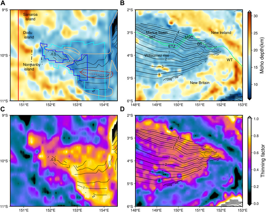
FIGURE 11. Distribution of Moho depth, thinning factor in the study area I and Ⅱ. The first column (A, C) is the two data distribution details of study area I; the second column is the data distribution details of study area Ⅱ. CBGA is the abbreviation of corrected Bouguer gravity anomaly. Previous research results are drawn in Figure 11A. The solid brown line represents the COB, where the dotted brown line is the spreading centre (Taylor et al., 1999). The solid orange line represents the oceanic crust since 1.2 Ma, where the dotted orange line is the spreading centre (Goodliffe and Taylor, 2022). The light blue solid line is the scope of the oceanic crust older than 0.73 Ma (Benes et al., 1994). The area surrounded by the dark blue line is the younger new-born oceanic crust, less than 0.73 Ma (Benes et al., 1997). The solid red line is the location of the receiver function line result of Abers et al. (2002). Martinez and Taylor. (1996) refer to the area enclosed by the solid green line in Figure 11B. ETZ represents the extensional transform zone. WiT, DT, and WT are transformed faults. The contours in the figures show the age of oceanic crust.

The oceanic crust displays apparent asymmetry on its northern and southern sides, with the southern side exhibiting a wider range and steeper inclination angle than the other one (Figure 11A). Abers et al. (2002) provided a north-south profile of Moho depth at the southwest corner of the WB using receiver function data at 150.8°E. We compared a portion of these results (9°S-11°S, the solid red line in Figure 11A) with our inversion results and the GEMMA model. We found that the inversion results fit the trend of the receiver function results more closely than the GEMMA model. The gravity inversion results match well with the receiver function results to the south direction from the point of coordinate (150.8°E, 10°S), with differences basically between 0 and 8 km. However, the Moho depth inversion results are generally lower than the receiver function results towards the south direction (>8 km) (Figure 12). This discrepancy may be caused by simple shear acting on the rift margin of the southern side of the lithosphere, resulting in a more complex geological structure on this side (Benes et al., 1994). Additionally, Taylor et al. (1999) provided the location of the Continent-Ocean Boundary (COB) (solid brown line in Figure 11A), which is situated in the narrow region between longitude 153°–154°5’ E on the south side of the oceanic crust, representing the boundary between the thinning continental crust and the normal oceanic crust. Meanwhile, the thinning factor is greater on the southern than on the northern side (>0.8, Figure 11C). These two pieces of evidence suggest the stronger tectonic movement on the southern side of the oceanic crust.

FIGURE 12

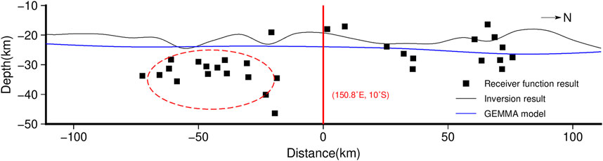
FIGURE 12. Comparison between the previous research results and this paper’s results at WB.

At 151°40′E, 9°–11°S, there are significant variations in crustal thickness and thinning factor, characterized by rapid crustal thickening (12–16 km) and drastic changes in thinning factor (0.8–0.3). Towards the west direction from 151°40′E, the terrain is transformed into a series of mounds and graben structures associated with continental rift (Benes et al., 1994) lies a narrow transition zone between seafloor spreading and continental rifting (Ferris et al., 2006), which is balanced by transition fault systems (Black dotted line in Figure 11A) (Benes et al., 1997).

Study area II is primarily situated in the Manus Basin (MB), which is bordered by New Ireland and New Britain. Receiver function analysis has determined a Moho depth point of 19.2 km at the Manus Islands (Xu et al., 2022), which is very close to our inversion results with a difference of only 0.4 km. The Manus spreading centre is located in the southeast corner of the MB, accompanied by an extensional transform zone to its left, together constituting the seafloor spreading segment. The relationship between continental rifting and seafloor spreading is balanced by three transform fault systems: WiT, DT, and WT (Martinez and Taylor, 1996). The crustal thickness in the MB and its vicinity remains relatively stable, primarily at 15 km. Moreover, the thinning factor is symmetrically distributed along the north and south sides of the spreading segment, indicating that the lithosphere may be uniformly stretched along the spreading part. Dyriw et al. (2021) also indicate that the back-arc crust was partially extended before seafloor spreading, suggesting that the spreading centre uniformly diffused along the spreading axis (Martinez and Taylor, 1996).

4.4 Microplates subduction and seismic activity

We select two profiles with distinct subduction features under the tectonic background and project the relative earthquakes within 150 km along with the profiles onto them to analyse the relationship between the Moho relief, earthquakes, and microplate subduction (Figures 7B, 13C, D).

FIGURE 13

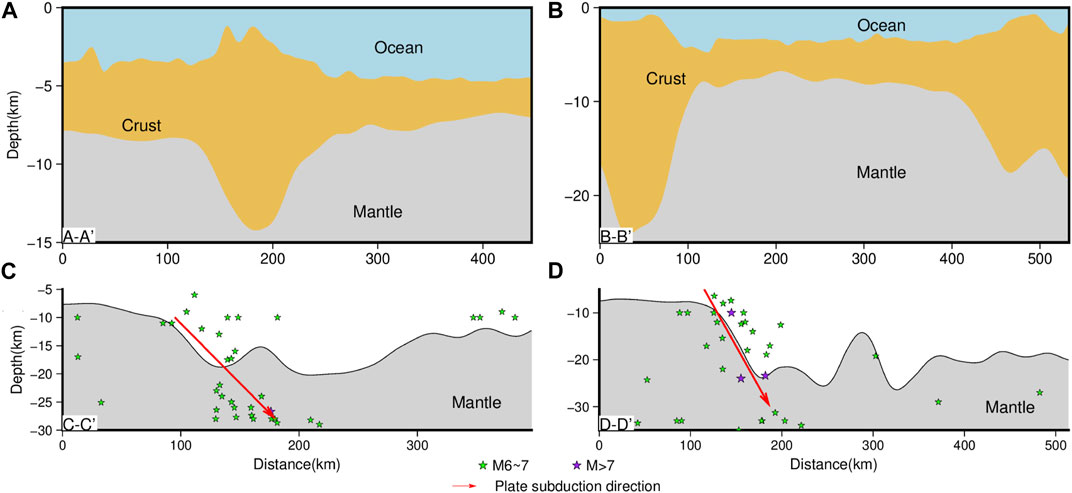
FIGURE 13. Four selected profiles, of which the locations of the profiles are shown in Figure 7B.

Profile C-C′ traverses the Western New Britain Trench, SSP, and BSP. The Australian Crustal front is embedded within a portion of the accretion block, influenced by arc-continent collision and block accretion. It provides upward heat flow (Holm and Richards, 2013), forming an active West Bismarck volcanic arc. In the first half of the profile, the Moho depth increases gradually from 10 km to 17 km; strong earthquakes are primarily distributed along the direction indicated by the red arrow (Figure 13C), which should be the angle of the SSP subducted beneath the BSP, severe subduction leads to the generation of fault systems in the deep crust (Abers, 1994).

Profile D-D’ across WB, East New Britain Trench, Solomon Islands, and Ontong Java Plateau shows that the Moho depth rapidly deepens from 8 to 23 km, and earthquakes are primarily distributed in the deep crust. The red arrow in Figure 13D may indicate the angle of WB subducted into the Solomon Islands. Therefore, we can assume that WB subducted into the Solomon Islands at a higher angle than SSP subducted beneath BSP according to Moho relief and earthquake distribution, which further suggests that the Solomon Islands are in a high-stress state, earthquakes on the west side of WB might be affected by it (Yoneshima et al., 2005).

Earthquakes are primarily concentrated in the Moho depth gradient zone of Papua New Guinea, particularly on both sides of the New Britain Trench. The lithosphere thinning factor varies significantly there, indicating intense stretching and strong deep crustal tectonic movement. Moreover, the anti-isostatic effect is most significant in the West New Britain Trench, demonstrating that underground materials’ distribution is exceptionally uneven and has a strong trend of isostatic adjustment (Yang et al., 2018), which may further trigger strong earthquakes.

In addition, the seismic distribution of SSP is mainly concentrated in the shallow crust. In contrast, the seismic distribution of BSP decreases gradually from shallow to medium-deep sources, which means BSP has lower integrity and is less stable than the former. Therefore, strong earthquakes near the West New Britain Trench tend to extend further under BSP with the development of microplate movement.

5 Conclusion

We discuss the characteristics of regional seafloor spreading and microplate subduction combined with other geophysical data from the perspective of the lithosphere thinning factor, Moho depth inversion result based on the gravity field model XGM 2019e by removing the lithosphere thermal gravity anomaly. The main conclusions are as follows:

(1) The Moho depth of Papua New Guinea is between 6 and 34 km. The lithosphere thinning factor is the largest at Solomon Sea Plate and Manus Islands, values at fragmented islands are close to 0. The maximum value of lithosphere thermal gravity anomaly is −200 mGal at Woodlark Basin.

(2) More intense tectonic movement occurred in the southern oceanic crust at the southwest of Woodlark Basin. Within Manus Basin, new oceanic crust expends uniformly on both sides along the spreading axis.

(3) The earthquakes and the Moho relief are closely related to microplate movement. Woodlark Basin subducted into the Solomon Islands at a higher Angle than Solomon Sea Plate beneath the Bismarck Sea Plate.

Data availability statement

The original contributions presented in the study are included in the article/supplementary material, further inquiries can be directed to the corresponding author.

Author contributions

YL contributed to the application of methods, original draft writing and review. GY, JZ, and BZ contributed to the draft review and its scientific development. All authors revised the manuscript and approved the final version for publication validation for the program. All authors contributed to the article and approved the submitted version.

Funding

This study was supported by the National Natural Science Foundation of China under Grant No. 42174104, U1939204 and Hubei Provincial Natural Science Foundation of China (2022CFB350).

Conflict of interest

The authors declare that the research was conducted in the absence of any commercial or financial relationships that could be construed as a potential conflict of interest.

Publisher’s note

All claims expressed in this article are solely those of the authors and do not necessarily represent those of their affiliated organizations, or those of the publisher, the editors and the reviewers. Any product that may be evaluated in this article, or claim that may be made by its manufacturer, is not guaranteed or endorsed by the publisher.

References

Abers, G. A., Ferris, A., Craig, M., Davies, H., Lerner-Lam, A. L., Mutter, J. C., et al. (2002). Mantle compensation of active metamorphic core complexes at Woodlark rift in Papua New Guinea. Nature 418 (22), 862–865. doi:10.1038/nature00990

PubMed Abstract | CrossRef Full Text | Google Scholar

Abers, G. A., and McCaffrey, R. (1994). Active arc-continent collision: Earthquakes, gravity anomalies, and fault kinematics in the Huon-Finisterre collision zone, Papua New Guinea. Tectonics 13 (2), 227–245. doi:10.1029/93TC02940

CrossRef Full Text | Google Scholar

Abrehdary, M., Sjöberg, L. E., and Bagherbandi, M. (2015). Combined Moho parameters determination using CRUST1.0 and vening meinesz-moritz model. J. Earth Sci. 26 (4), 607–616. doi:10.1007/s12583-015-0571-6

CrossRef Full Text | Google Scholar

Aitken, A. R. A. (2010). Moho geometry gravity inversion experiment (MoGGIE): A refined model of the Australian Moho, and its tectonic and isostatic implications. Earthpl. Sci. Lett. 297, 71–83. doi:10.1016/j.epsl.2010.06.004

CrossRef Full Text | Google Scholar

Aitken, A. R. A., Salmon, M. L., and Kennett, B. L. N. (2013). Australia's Moho: A test of the usefulness of gravity modelling for the determination of Moho depth. Tectonophysics 609, 468–479. doi:10.1016/j.tecto.2012.06.049

CrossRef Full Text | Google Scholar

Alvey, A., Gaina, C., Kusznir, N. J., and Torsvik, T. H. (2008). Integrated crustal thickness mapping and plate reconstructions for the high Arctic. Earthpl. Sci. Lett. 274 (3-4), 310–321. doi:10.1016/j.epsl.2008.07.036

CrossRef Full Text | Google Scholar

Amante, C., and Eakins, B. W. (2009). “ETOPO1 1 arc-minute global relief model: Procedures, data sources and analysis,” in NOAA technical memorandum NESDIS NGDC-24 (National Geophysical Data Center, NOAA). doi:10.7289/V5C8276M

CrossRef Full Text | Google Scholar

Benes, V., Bocharova, N., Popov, E., Scott, S. D., and Zonenshain, L. (1997). Geophysical and morpho-tectonic study of the transition between seafloor spreading and continental rifting, Western Woodlark Basin, Papua New Guinea. Mar. Geol. 142, 85–98. doi:10.1016/S0025-3227(97)00042-X

CrossRef Full Text | Google Scholar

Benes, V., Scott, S. D., and Binns, R. A. (1994). Tectonics of rift propagation into a continental margin: Western Woodlark Basin, Papua New Guinea. J. Geophys. Res. Solid Earth 99 (B3), 4439–4455. doi:10.1029/93JB02878

CrossRef Full Text | Google Scholar

Bird, P. (2003). An updated digital model of plate boundaries. Geochem. Geophys. Geosystems 4 (3), 1027. doi:10.1029/2001GC000252

CrossRef Full Text | Google Scholar

Borrero, J. C., Bu, J., Saiang, C., UsJu, B., Freckman, J., Gomer, B., et al. (2003). Field Survey and preliminary modeling of the wewak, Papua New Guinea earthquake and tsunami of 9 september 2002. Seismol. Res. Lett. 74 (4), 393–405. doi:10.1785/gssrl.74.4.393

CrossRef Full Text | Google Scholar

Bown, J. W., and White, R. S. (1994). Variation with spreading rate of oceanic crustal thickness and geochemistry. Earthpl. Sci. Lett. 121, 435–449. doi:10.1016/0012-821X(94)90082-5

CrossRef Full Text | Google Scholar

Chappell, A. R., and Kusznir, N. J. (2008). Three-dimensional gravity inversion for Moho depth at rifted continental margins incorporating a lithosphere thermal gravity anomaly correction. Geophys. J. Int. 174, 1–13. doi:10.1111/j.1365-246X.2008.03803.x

CrossRef Full Text | Google Scholar

Constantino, R. R., and Sacek, V. (2020). Thermal correction for Moho depth estimations on west philippine basin: A Python code to calculate the gravitational effects of lithospheric cooling under oceanic crust. Pure Appl. Geophys 177, 5225–5236. doi:10.1007/s00024-020-02581-2

CrossRef Full Text | Google Scholar

Cowie, L., and Kusznir, N. (2012). Gravity inversion mapping of crustal thickness and lithosphere thinning for the eastern Mediterranean. Lead. Edge 31 (7), 810–814. doi:10.1190/tle31070810.1

CrossRef Full Text | Google Scholar

Curtis, J. W. (1973). Plate tectonics and the papua—new Guinea—Solomon islands region. J. Geol. Soc. Aust. 20 (1), 21–35. doi:10.1080/14400957308527892

CrossRef Full Text | Google Scholar

Davies, H. L. (2012). The geology of New Guinea - the cordilleran margin of the Australian continent. Episodes 35 (1), 87–102. doi:10.18814/epiiugs/2012/v35i1/008

CrossRef Full Text | Google Scholar

Dyriw, N. J., Bryan, S. E., Richards, S. W., Parianos, J. M., Arculus, R. J., and Gust, D. A. (2021). Morphotectonic analysis of the east Manus Basin, Papua New Guinea. Front. Earth Sci. 8, 596727. doi:10.3389/feart.2020.596727

CrossRef Full Text | Google Scholar

Ferris, A., Abers, G. A., Zelt, B., Taylor, B., and Roecker, S. (2006). Crustal structure across the transition from rifting to spreading: The Woodlark rift system of Papua New Guinea. Geophys. J. Int. 166, 622–634. doi:10.1111/j.1365-246X.2006.02970.x

CrossRef Full Text | Google Scholar

Gaulier, J. M., Chamot-Rooke, N., and Jestin, F. (1997). Constraints on Moho depth and crustal thickness in the Liguro-Provençal Basin from a 3d gravity inversion: Geodynamic implications. Rev. l’Institut Français Pétrole, EDP Sci. 52 (1), 557–583. doi:10.2516/ogst:1997060

CrossRef Full Text | Google Scholar

Goodliffe, A. M., and Taylor, B. (2022). The boundary between continental rifting and sea-floor spreading in the Woodlark Basin, Papua New Guinea. Geol. Soc. Spec. Publ. 282, 217–238. doi:10.1144/sp282.11

CrossRef Full Text | Google Scholar

Greenhalgh, E. E., and Kusznir, N. J. (2007). Evidence for thin oceanic crust on the extinct Aegir Ridge, Norwegian Basin, NE Atlantic derived from satellite gravity inversion. Geophys. Res. Lett. 34, L06305. doi:10.1029/2007GL029440

CrossRef Full Text | Google Scholar

Haddad, D., and Watts, A. B. (1999). Subsidence history, gravity anomalies, and flexure of the northeast Australian margin in Papua New Guinea. Tectonics 18 (5), 827–842. doi:10.1029/1999TC900009

CrossRef Full Text | Google Scholar

Holm, R. J., and Richards, S. W. (2013). A re-evaluation of arc–continent collision and along-arc variation in the Bismarck Sea region, Papua New Guinea. Aust. J. Earth Sci. 60 (5), 605–619. doi:10.1080/08120099.2013.824505

CrossRef Full Text | Google Scholar

Honza, E., Davies, H. L., Keene, J. B., and Tiffin, D. L. (1987). Plate boundaries and evolution of the Solomon sea region. Geo-Mar Lett. 7, 161–168. doi:10.1007/BF02238046

CrossRef Full Text | Google Scholar

Joshima, M., Okuda, Y., Murakami, F., Kishimoto, K., and Honza, E. (1987). Age of the Solomon sea basin from magnetic lineations. Geo-Mar Lett. 6, 229–234. doi:10.1007/BF02239584

CrossRef Full Text | Google Scholar

Mann, P., Taylor, F. W., Lagoe, M. B., Quarles, A., and Burr, G. (1998). Accelerating late Quaternary uplift of the New Georgia Island Group (Solomon island arc) in response to subduction of the recently active Woodlark spreading center and Coleman seamount. Tectonophysics 295, 259–306. doi:10.1016/S0040-1951(98)00129-2

CrossRef Full Text | Google Scholar

Martinez, F., and Taylor, B. (1996). Backarc spreading, rifting, and microplate rotation, between transform faults in the Manus Basin. Mar. Geophys. Res. 18, 203–224. doi:10.1007/BF00286078

CrossRef Full Text | Google Scholar

Mckenzie, D. (1978). Some remarks on the development of sedimentary basins. Earth Planet. Sci. Lett. 40, 25–32. doi:10.1016/0012-821X(78)90071-7

CrossRef Full Text | Google Scholar

Müller, D. R., Zahirovic, S., Williams, E. S., Cannon, J., Seton, M., Bower, D. J., et al. (2019). A global plate model including lithospheric deformation along major rifts and orogens since the Triassic. Tectonics 38, 1884–1907. doi:10.1029/2018TC005462

CrossRef Full Text | Google Scholar

Pigram, C. J., and Davies, H. L. (1987). Terrranes and the accretion history of the new Guinea orogen: Bmr. J. Aust. Geol. Geophys. 10, 193–211.

Google Scholar

Reguzzoni, M., and Sampietro, D. (2015). Gemma: An Earth crustal model based on GOCE satellite data. Int. J. Appl. Earth Obs. Geoinf 35 (A), 31–43. doi:10.1016/j.jag.2014.04.002

CrossRef Full Text | Google Scholar

Silva, J., Medeiros, W., and Barbosa, V. (2001). Potential-field inversion: Choosing the appropriate technique to solve a geologic problem. Geophysics 66 (2), 511–520. doi:10.1190/1.1444941

CrossRef Full Text | Google Scholar

Silva, J., Santos, D., and Gomes, K. (2014). Fast gravity inversion of basement relief. Geophysics 79 (5), G79–G91. doi:10.1190/geo2014-0024.1

CrossRef Full Text | Google Scholar

Taylor, B., Goodliffe, A. M., and Martinez, F. (1999). How continents break up: Insights from Papua New Guinea. J. Geophys. Res. Solid Earth 104 (B4), 7497–7512. doi:10.1029/1998JB900115

CrossRef Full Text | Google Scholar

Uieda, L., Barbosa, V. C. F., and Braitenberg, C. (2015). Tesseroids: Forward-modeling gravitational fields in spherical coordinates. Geophysics 81 (5), 41–48. doi:10.1190/geo2015-0204.1

CrossRef Full Text | Google Scholar

Uieda, L., and Barbosa, V. C. F. (2017). Fast nonlinear gravity inversion in spherical coordinates with application to the South American Moho. Geophys. J. Int. 208, 162–176. doi:10.1093/gji/ggw390

CrossRef Full Text | Google Scholar

Wallace, L. M., Stevens, C., Silver, E., McCaffrey, R., Loratung, W., Hasiata, S., et al. (2004). GPS and seismological constraints on active tectonics and arc-continent collision in Papua New Guinea: Implications for mechanics of microplate rotations in a plate boundary zone. J. Geophys. Res. Solid Earth 109 (B05404), 1–16. doi:10.1029/2003JB002481

CrossRef Full Text | Google Scholar

White, R., and Mckenzie, D. (1989). Magmatism at rift zones: The generation of volcanic continental margins and flood basalts. J. Geophys. Res. Solid Earth 94 (86), 7685–7729. doi:10.1029/JB094iB06p07685

CrossRef Full Text | Google Scholar

Wu, Z. C., Gao, J. Y., Ding, W. W., Shen, Z. Y., Zhang, T., and Yang, C. G. (2017). Moho depth of the South China Sea basin from three-dimensional gravity inversion with constraint points. Chin. J. Geophys. 60 (4), 368–383. doi:10.6038/cjg20170709

CrossRef Full Text | Google Scholar

Xu, C., Xing, J. H., Gong, W. W., Zhang, H., Xu, H. W., and Xu, X. (2022). Density structure of the Papua New Guinea-Solomon arc subduction system. J. Ocean. Univ. China 22 (3), 1–8. doi:10.1007/s11802-023-5425-8

CrossRef Full Text | Google Scholar

Xu, Z., Feng, W. P., Du, H. L., Li, L., Wang, S., Yi, L., et al. (2020). The 2018 M_<i>w</i> 7.5 Papua New Guinea earthquake: A possible complex multiple faults failure event with deep-seated reverse faulting. Geophys. Res. Lett. 47, e2020GL089271. doi:10.1029/2019EA000966

CrossRef Full Text | Google Scholar

Yang, G. L., Shen, C. Y., Wang, J. P., Xuan, S. B., Wu, G. J., and Tan, H. B. (2018). Isostatic anomaly characteristics and tectonism of the New Britain Trench and neighboring Papua New Guinea. Geod. Geodyn. 9 (5), 404–410. doi:10.1016/j.geog.2018.04.006

CrossRef Full Text | Google Scholar

Yoneshima, S., Mochizuki, K., Araki, E., Hino, R., Shinohara, M., and Suyehiro, K. (2005). Subduction of the Woodlark Basin at new Britain trench, Solomon islands region. Tectonophysics 397, 225–239. doi:10.1016/j.tecto.2004.12.008

CrossRef Full Text | Google Scholar

Zhu, L. P., and Kanamori, H. (2000). Moho depth variation in southern California from teleseismic receiver functions. J. Geophys. Res. Solid Earth 105 (B2), 2969–2980. doi:10.1029/1999JB900322

CrossRef Full Text | Google Scholar

Zingerle, P., Pail, R., Gruber, T., and Oikonomidou, X. (2020). The combined global gravity field model XGM2019e. J. Geod. 94 (7), 66. doi:10.1007/s00190-020-01398-0

CrossRef Full Text | Google Scholar