 Shunzhi He
 Xiaoping Cheng1*
 Xiangcheng Li
 Zexun Wei
 Xiaogang Huang
95% of researchers rate our articles as excellent or good
Learn more about the work of our research integrity team to safeguard the quality of each article we publish.
Find out more
ORIGINAL RESEARCH article
Front. Earth Sci. , 13 March 2023
Sec. Atmospheric Science
Volume 11 - 2023 | https://doi.org/10.3389/feart.2023.1142537
The cold wake caused by a tropical cyclone (TC) extends for hundreds of kilometers and persists for several weeks, thus influencing the surface response for any subsequent TCs that might pass over it. It is commonly accepted that sea-surface temperature (SST) cooling, as produced by a single TC, occurs primarily through vertical mixing. However, when there are sequential TCs, the earlier TC can dramatically change the thermal structure of the upper ocean, which may influence the subsequent development of a latter-occurring TC (LTC). Therefore, the contribution of horizontal advection and vertical mixing to SST-cooling during the passage of LTCs is of great interest. Using a 19-year-long observational dataset and the heat budget analysis of an idealized numerical simulation, the SST change during the passage of sequential TCs is investigated. The results demonstrate that, on average, the SST cooling caused by the LTC shows an overall decreasing trend with enhanced lingering wakes. Budget analysis of the model simulations suggests that an earlier TC can suppress the vertical mixing induced by an LTC mainly through an alteration of dynamics within the deepened mixed layer and that the contribution of vertical mixing to the SST cooling is weaker due to the intensification of the earlier TC. The weakened vertical mixing dominates the decreased SST cooling induced by an LTC. In contrast, the cold wake generated by an earlier TC can produce more cold water on the right side of the TC’s track, which contributes to stronger horizontal advection upon the arrival of the LTC. In general, the effects of the earlier TC can suppress the sea-surface thermal response to an LTC. If the contribution of the horizontal advection to SST cooling is neglected, the SST cooling induced by an LTC could be reduced by about 40%. As for the response of the sub-surface water to the passage of an LTC, the weakened warm anomaly induced by vertical mixing and the enhanced cooling anomaly caused by the vertical advection explain the reduced tendency for the mixed layer to deepen. As a result, the tendency for the mixed layer depth (MLD) to increase is suppressed during the passage of an LTC. These results highlight the importance of optimally depicting cold wakes in numerical simulations to improve the prediction of the upper ocean’s response to sequential TCs.
Tropical cyclones (TCs) with strong surface wind can produce one of the most severe natural disasters in the tropics and subtropics. They can also impact upper-ocean dynamics. During the passage of a single TC, the surface wind stress can significantly disturb the upper-ocean structure. A notable feature of this response is sea-surface temperature (SST) cooling, particularly on the right side of the TC track in the Northern Hemisphere (Price et al., 1994). The TC-induced SST cooling ranges from less than 1°C to greater than 10°C (Cione et al., 2000; Lin et al., 2003; Chiang et al., 2011; Dare and McBride, 2011; Baranowski et al., 2014). Tropical cyclones can change the SST mainly through three processes: vertical mixing, upwelling, and air-sea flux exchange (Zhang et al., 2018; Liu et al., 2019). The vertical mixing is produced by wind-induced current velocity shear, which is an associated entrainment process in the upper ocean (Shay et al., 2000; Jaimes and Shay, 2009). Many studies found that TC-induced vertical mixing leads to SST cooling (up to ∼85%). The upwelling process, which brings cold sub-surface water to the surface ocean, is caused by the near-inertial oscillation and wind-driven Ekman pumping effect (Huang et al., 2009; Zhang et al., 2019) and contributes less than 15% to SST cooling (Price, 1981). In addition to vertical mixing and upwelling, air-sea turbulent flux exchanges (sensible heat and latent heat) also influence the SST. Still, it is not as important as the two major oceanic processes (Jacob et al., 2000). Besides SST cooling, the sub-surface water temperature is modulated by mixing, vertical advection (upwelling and downwelling), and horizontal advection (Yang et al., 2015; Chen et al., 2020). Mixing can warm the sub-surface water, resulting in the deepening of the oceanic mixed layer. Vertical advection brings the cold water of thermocline into the mixed layer through upwelling, weakening the warm sub-surface anomaly or even turning it into a cold anomaly (Niwa and Hibiya, 1997; Wu and Li, 2018; Zhang et al., 2018). As a result of the mixing, the sub-surface water can be warmed by up to 4°C and can usually be modulated by vertical advection (Zhang et al., 2016; Zhang et al., 2019).
The upper-ocean response to TCs strongly depends not only on both the intensity and translation speed but also on pre-existing oceanic background environments, such as warm-core eddies, cold-core eddies, and the western boundary current (Lin et al., 2008; Lin et al., 2009; Uhlhorn and Shay, 2013; Wei et al., 2014; Wang et al., 2016; Lin et al., 2017; Ma et al., 2018). Several case studies found that weak upper-ocean cooling occurred in the warm-core eddy during a TC passage (Shay et al., 2000; Lin et al., 2005; Jaimes and Shay, 2009; Jaimes and Shay, 2010; Vianna et al., 2010). They attributed this to the characteristic deep thermocline and the negative vorticity within the warm-core eddy. The positive vorticity and the shallow mixed layer in the cold-core eddies contribute to upper-ocean cooling during the passage of a TC (Ma et al., 2017). Based on the satellite data, Walker et al. (2005, 2014) found that SST cooling has been observed to amplify to 3°C–9°C when TCs pass over a cold-core eddy regime. Wu et al. (2008) found that no significant temperature cooling occurred in the Kuroshio because of a thick mixed layer. Meanwhile, previous studies on a TC passing over the Kuroshio and Gulf Stream found that the surface and sub-surface water experienced a rapid temperature recovery because of downstream transport by strong sea currents (Uhlhorn and Shay, 2013; Liu and Wei, 2015; He et al., 2022).
Except for the oceanic eddy and the western boundary current, the cold wake left behind by a TC is also a common feature, which would significantly change the thermal structure of the upper ocean. The cold wake may extend for hundreds of kilometers adjacent to the storm track in the horizontal direction and persist for several weeks after the passage of a TC, influencing the upper-ocean response to subsequent or latter TCs (hereafter referred to as LTCs) passing over it within several weeks. (Price et al., 2008; Balaguru et al., 2014; Walker et al., 2014). Based on numerical simulations, Baranowski et al. (2014) suggested that the magnitude of the SST response to sequential TCs (Jangmi and Hagupit) was larger than that caused by a single TC (Jangmi). Wu and Li (2018) claimed that the magnitude of SST cooling is significantly larger when the upper ocean is influenced by successive TCs within a short period. In addition, the SST response to an LTC would have been significantly larger if the ocean had not already been influenced by an earlier TC (hereafter referred to as, ETC) (Baranowski et al., 2014). Due to the deeper mixed layer (MLD) produced by an, ETC, LTC-induced SST cooling (∼2°C), as indicated by satellite SST maps, was found to be weaker than that caused by an, ETC (∼4°C) (Zhang et al., 2019).
The upper ocean response to a single TC has been well documented in previous studies, while less is known about the upper ocean response to successive TCs. The state and structure of the upper ocean play a crucial role in the intensification of TCs. Thus it is essential to understand the effect of the, ETC., on the upper ocean response to sequential TCs. The existing literatures has focused on an individual case about the upper ocean response to sequential TCs. It is unclear to what extent the conclusions from those studies suitably apply to most cases concerning the upper-ocean response to sequential TCs. Based on a statistical analysis of observational data and idealized numerical simulations, this study aims to investigate the upper ocean response to the sequential TCs passing over the Western North Pacific. The remainder of this paper is organized as follows: The data, statistical methods, and model configuration are presented in Section 2. The results of statistical analysis and numerical simulations are shown in Section 3. Section 4 presents a summary.
The data used in this study include the positions and intensities of the TCs, satellite-derived SST maps, and climatological oceanic temperature and salinity. The TC best track data is from the Joint Typhoon Warning Center (JTWC; https://www.metoc.navy.mil/jtwc), which includes the TC’s center position, the maximum sustained surface wind speed, the radius of the 34 kt and 50 kt surface wind, and the minimum sea level pressure at 6-h intervals. The location of the TC center is based on the 6-h best track data before TC landfall. The daily SST dataset, provided by Remote Sensing Systems (https://www.remss.com/measurements/), has a high spatial resolution of 0.25°in both latitude and longitude. This data set is produced by combining the microwave-observed SST data from the Microwave Imager of Tropical Rainfall Measuring Mission, Advanced Microwave Scanning Radiometer for EOS AMSR-E, and the Advanced Microwave Scanning Radiometer 2. The Argo data are used to obtain the MLD characteristics, which consist of a delayed mode and quality-controlled data (https://argo.ucsd.edu/data/). The climate temperature and salinity data were obtained from the National Centers for Environmental Information (World Ocean Atlas 2018: https://www.ncei.noaa.gov/products/world-ocean-atlas). To be consistent with the available ocean variables, the TC track data from 2002 to 2020 were selected.
To investigate the ocean response to sequential TCs, TC tracks were required to determine the important parameters, which are “closeness in time” and “closeness in space” (Balaguru et al., 2014). The maximum time difference between an, ETC., track and an LTC track may be as long as 14 days since the mean recovery time required for SST cooling is statistically close to 2 weeks (Ma et al., 2018; He et al., 2022). The mean radius of 12 m/s surface wind for cyclones in Northern west Pacific is about 250 km (Chavas and Emanuel, 2010). In this study, the mean radius of the 12 m/s surface wind selected as the metric is refererd to the study of Baranowski et al. (2014), which claimed that little deep convection occurs beyond this distance.
To describe the temporal characteristics of the local SST response to sequential TCs, day 0 refers to the arrival day of the LTC. The time window begins 12 days before the passage of the, ETC., and extends to 30 days after the LTC passage (Lloyd and Vecchi, 2010; Mei and Pasquero., 2013). At first, the values of ocean variables at each location are computed through subtracting climatological values of daily ocean variables for the removal of the seasonal cycle and the long-term trend. Then the SST cooling was calculated at the fixed point of the TC center by the difference between the instantaneous SSTs and the mean SST values from 12 to 3 days before the, ETC., passage. In the meanwhile, we removed the TC records including more than 2 TCs. Thus, aA total of 11,704 TC center records passing over the domain bounded by 100–180°E, 0–40°N were obtained. Including 10,901 single TC track records and 803 sequential TCs track records. All records were composited based on the time relative to the passage of the TC to investigate the temporal characteristics of the upper-ocean thermal response to TCs.
To better interpret the mechanisms of the SST response to sequent TCs, the Coastal and Regional Ocean Community model (CROCO)was used for numerical simulations with different idealized TC and oceanic fields (Ezer et al., 2000). The model was successfully used in previous studies to simulate and explore the physical processes involved in the ocean response to a TC (Jullien et al., 2014). Here the model domain spanned 4,000 km in the x-direction and 6,000 km in the y-direction, with a 15 km horizontal resolution. The model bathymetry was set as 1,500 m for the entire model domain. There are 35 terrain-following vertical levels with a finer layer distribution in the upper 100 m to better resolve the ocean mixed layer. The generic length scale method with the k−ε closure scheme (Warner et al., 2005) was implemented for parameterization of the ocean vertical turbulent mixing. In an effort to choose a representative profile of the oceanic state, the mean temperature and salinity profiles from the WOA18 climatology data were calculated for the domain of 130°–180°E, 10°-25°N during the TC season (from August to October). As shown in Figures 1C, D, the selected domain and time are based on the observation. Finally, according to the average profile (Figure 2), the initial salinity and temperature field on the whole domain was set as horizontally homogeneous. The current velocity was set to zero, and thus the model ocean was initially at rest.
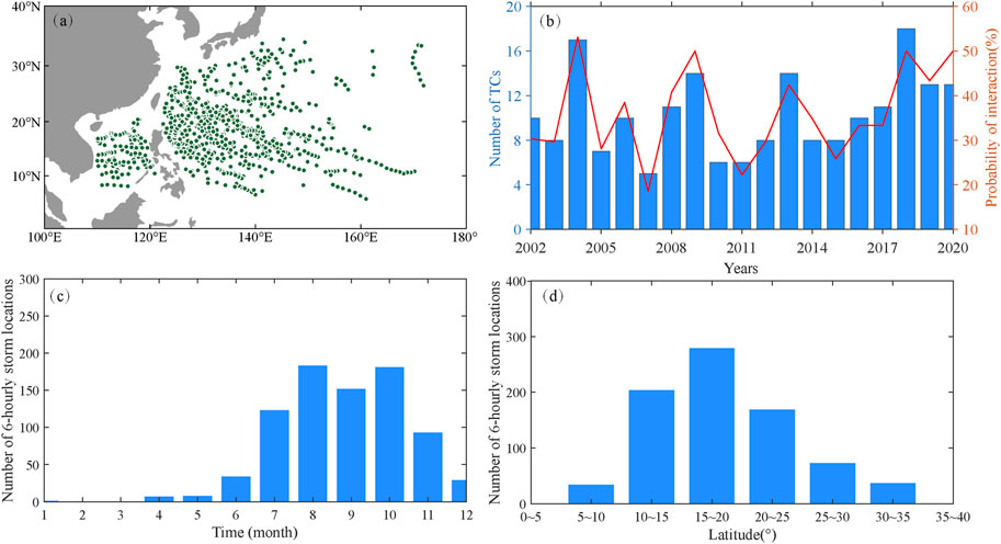
FIGURE 1. (A) A spatial map of the distributions for cyclones when they encountered cold wakes from 2002 to 2020. (B) The interaction probability for cyclones when they encountered cold wakes and the number of cyclones for each year. (C) The number of 6-hourly cyclone track locations for each month. (D) The number of 6-hourly cyclone track locations for each latitude.
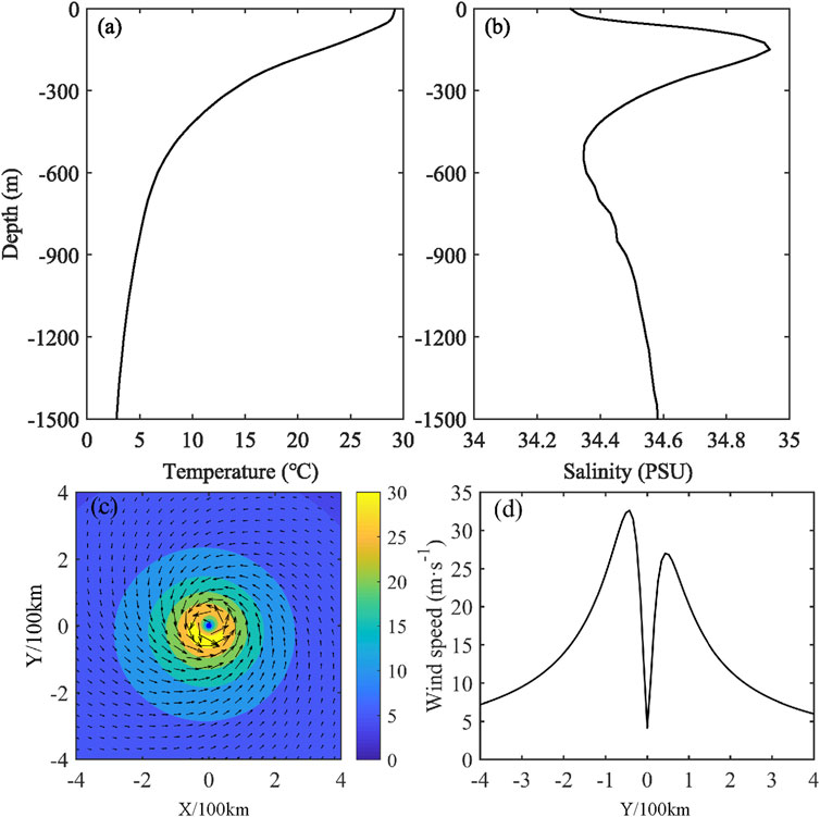
FIGURE 2. (A) Temperature and (B) Salinity for the WOA18 profiles averaged over the domain of 130°–180°E, 10°-25°N during the TC season (from August to October). These were used as initial conditions for CROCO model. (C) The reconstructed vector wind field of idealized TC based on the SLOSH method, with color shading for wind speed. (D) Idealized wind speed across TC center and along the y direction.
The ocean model was forced by the surface wind of an idealized moving TC, with a translation speed of 6 m/s. The idealized axisymmetric wind field is constructed according to the Sea Lake and Overland Surges from Hurricanes method (Jelesnianski, 1966; Jelesnianski and Taylor, 1973). The wind forcing for the model has asymmetries due to the translation speed of the TC (Figures 2C, D). This model defined the wind speed as follows:
where Vmax is the maximum wind speed (m/s), Rmax is the radius (m) of the maximum wind speed, and r is the distance (m) from the center of the TC.
Based on the 19-year JTWC data, the mean maximum surface wind speed for the LTC was 35 m/s, which was used for the idealized wind forcing in this study. The radius of maximum wind was set as 50 km, as shown in Figures 2C, D. The surface enthalpy flux under the corresponding TC condition was obtained and considered as model forcing. Similar to what has been in some previous studies (e.g., Jaimes et al., 2015; Gelaro et al., 2017; Jeon et al., 2022), the surface enthalpy flux (sum of sensible and latent heat fluxes) under the corresponding TC condition were calculated in the typhoon region using the following bulk formula:
where
The CROCO model was integrated for a total of 15 days. To characterize the processes responsible for the thermal response, a heat budget analysis was carried out with the following thermodynamic equation at each model grid point (Wei et al., 2014; Li et al., 2022):
Here, the left-hand term is the local tendency of temperature (RATE), and the terms on the right-hand side are the horizontal advection term (HADV), vertical advection term (VADV), horizontal diffusion term (HDIF), and vertical mixing term (VMIX), respectively. In general, for SST cooling, the contribution of the HDIF was much smaller than the VMIX and ADV; thus, they were neglected in this study.
The spatial and temporal distribution of sequential TCs tracks over the Western North Pacific from 2002 to 2020 is given in Figure 1. There are a total of 540 TCs, of which 33% have sequential TC tracks. Figure 3 shows the probability density function of the maximum SST anomaly. The maximum SST cooling at each point was obtained based on the temporal evolution of SST anomaly from −12 days relative to the passage of the, ETC., to +30 days relative to the LTC passage. Whether there was an, ETC., or not, the shape of probability density function is similar, whereas the maxima of the probability density function are different (Figure 3A). The peak probability for the SST anomaly induced by a sequential TC is found to be approximately −0.5°C smaller than that generated by a single TC. Compared with the single-TC condition, the probability is smaller (larger) under the sequential-TC condition when SST anomalies is weaker (stonger) than −1°C. Figure 3B shows that the mean maximum SST cooling in the sequential-TC condition is −1.50°C, which is 0.16°C colder than that in the single-TC condition. This difference is significant above the 95% confidence level based on a Student’s t-test. This suggests that sequential TCs can amplify a TC-induced SST response.
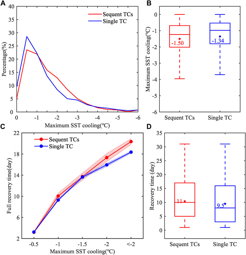
FIGURE 3. (A) Probability density function and (C) The recovery time as a function of maximum SST cooling. Boxplots of maximum SST cooling (B) and recovery time (D). In subgraph (B) and (D), the dots in boxes denote the averaged values. The larger maximum SST cooling in the sequent TCs condition than that in the single TC condition is significant above the 95% confidence level based on the Student’s t-test. The increase of recovery time under the sequential TCs condition compared to that under the single TC condition is significant above the 95% confidence level based on the Student’s t-test.
After the SST cooling reaches its peak value, it is followed by a subsequent relaxation period with the departure of the TC. During the relaxation stage, the sea surface absorbs heat through air-sea heat flux, and the SST recovers. The recovery time for the SST to return to the pre-TC state ranges from 1 day to more than 30 days (Hart et al., 2007; Price et al., 2008). Within 30 days after the TC’s passage, some data points for the SST may not have fully recovered, and those points are discarded in the analysis. As shown in Figure 3C, the mean recovery time for a sequential-TC condition is 11 days, longer than that for a single TC, with a difference of 1.5 days. The difference is significant above the 95% confidence level based on a Student’s t-test. As shown in Figure 3D, the mean recovery time is computed according to the maximum cooling at an interval of 0.5°C. Given the same SST cooling, there is no difference between the conditions of sequential TCs and a single TC, as shown in Figure 3D. This indicates that sequential TCs prolong the recovery time of the SST, which is intuitive, as it should take longer to recover from cooler conditions.
The characteristics of the SST response to a TC are affected by the TC intensity and translation speed (Samson et al., 2009; Wang et al., 2016; Lin et al., 2017). The correlation coefficients between the maximum SST cooling and the intensity of TCs are calculated. When TCs do not encounter the ETC-induced cold wake, the correlation coefficient is −0.49 (Figure 4). In contrast, a correlation coefficient of −0.41 is slightly weaker when TCs encounter the ETC-induced cold wake. Similarly, without a cold wake, the correlation coefficient between the maximum SST cooling and translation speed of TC is 0.26, substantially larger than that when TCs encounter the ETC-induced cold wake, which is 0.18. The ETC-induced cold wake reduces the correlation between the TC (intensity and translation speed) and the maximum SST cooling. Thus, the maximum SST cooling may also be affected by the ETC-induced cold wake, except for the intensity and translation speed of the TC.
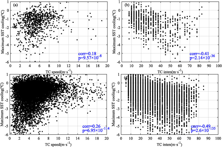
FIGURE 4. Scatterplots of the maximum SST cooling and the (A) speed and (B) intensity of the LTC at each 6-h location. Scatterplots of the maximum SST cooling and the (C) speed and (D) intensity of the single TC at each 6-h location. Numbers in each plot indicate the correlation coefficients and p-vaule. These correlation coefficients are statistically significant (p<0.0001).
To further explore the effect of the ETC-induced cold wakes in the maximum SST cooling, the maximum SST cooling induced by the sequential TC is separated into two parts: (1) the ETC-induced SST cooling (the remnant of the cold wake) and (2) the LTC-induced SST cooling. Due to the large wind field of TC, the SST begins to decrease one or 2 days before the arrival of a TC (Dare and McBride, 2011). Therefore, for time difference between an, ETC., track and an LTC track more than 2 days, the ETC-induced SST cooling is defined as the SSTA observed 3 days before the LTC passage. As for time difference between an, ETC., track and an LTC track less than 3 days, the ETC-induced SST cooling is defined as the SSTA observed at, ETC., arrvial. Noting that the ETC-induced SST cooling did not represent the ETC-induced maximum cooling, but the remnant of the ETC-induced cold wake. The LTC-induced SST cooling is calculated by subtracting the ETC-induced SST cooling from the maximum SST cooling induced by sequential TCs. The mean LTC-induced SST cooling is −1.08°C, substantially stronger than the mean ETC-induced SST cooling, which was −0.42°C. In addition, the TC-induced SST cooling difference between a single TC and an LTC can be clearly seen in Figures 3B, 5A, and it is significant above a 95% confidence level based on a Student’s t-test. These results suggest that the ETC-induced cold wake can contribute to a larger SST response associated with the passage of sequential TCs, but inhibit the LTC-induced SST response. In addition, the effect of an ETC-induced cold wake on the LTC-induced SST cooling and sequential TCs is more significant, with the ETC-induced cold wake intensifying (Figures 5B, C).
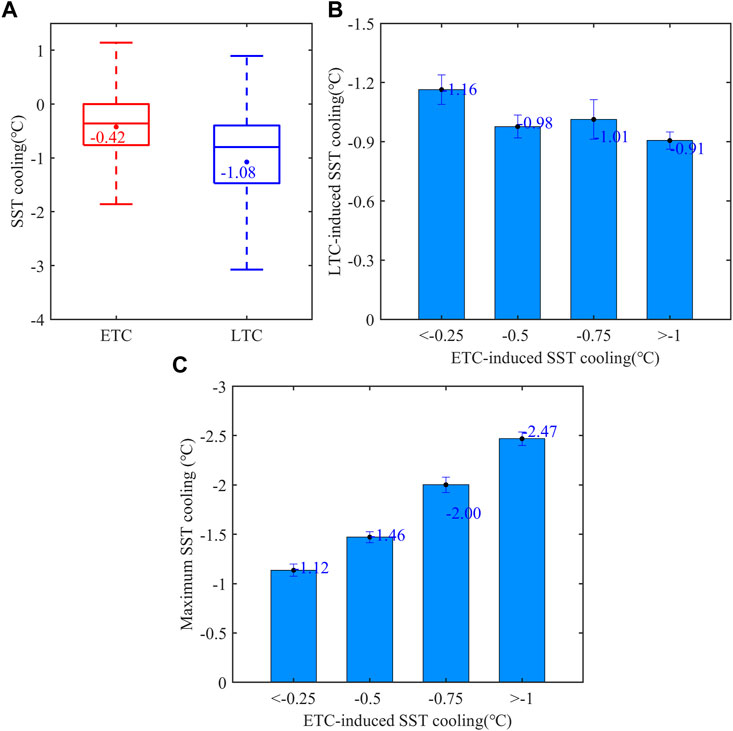
FIGURE 5. The boxplot of the ETC-induced SST cooling and the LTC-induced SST cooling (A) during the passage of sequential TCs and (B) the mean SST cooling induced by the LTC and the sequential TCs and (C) as a function of the ETC-induced SST cooling. In subgraph (A), the dots in the boxes denote the average values of SST cooling. The degree to which the LTC-induced SST cooling is larger than the ETC-induced SST cooling is significant above the 95% confidence level based on the Student’s t-test.
In addition, we the Argo float profiles within 150 km around the TC center recording according to the time change. Based on the Argo data, the mixed layer was also been analyzed under the sequential-TC condition (Figure 6). The MLD is defined as the depth where the density had increased by 0.125 kg m−3 above the value of the surface density (Girishkumar et al., 2004; Ye et al., 2019). The MLD remarkably deepened due to the stirring action of a TC, it is consistent with the previous studies (Mei and Pasquero, 2013; Zhang et al., 2016). When there are sequential TCs, the MLD has a two successive deepening (Zhang et al., 2019). For the first deepening induced by the, ETC, the ETC-indcued MLD anomaly is larger on 4 days before the LTC passage than that under the single TC condition. As shown in Figure 6B, the, ETC., has a mean TC intensity 30.03 m s−1, compared to 27.05 m s−1 of the single TC. This difference is significant above the 95% confidence level based on Student’s t-test. However, The differences between the, ETC., and the single TC in translation speed are insignificant based on the Student’s t-test (Figure 6C). These suggest that the ETC-induced MLD anomaly is larger than that produced by the single TC. As shown in Figure 6A, the MLD anomaly under the sequential TCs condition is deepened to 11 m, which is deeper than that in the single TC condition by 4 m. It may be explained by the fact that the upper ocean is exposed to more wind energy from the sequential TCs.
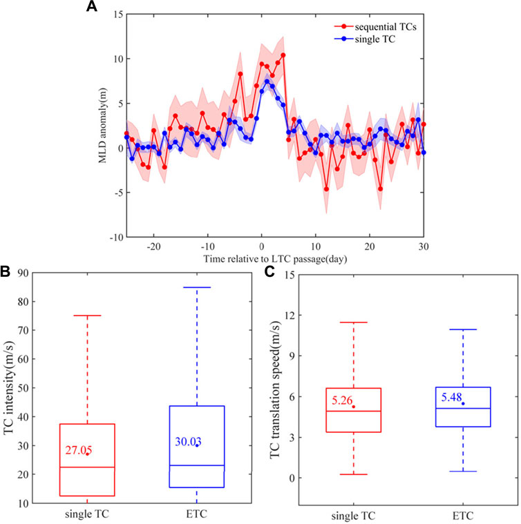
FIGURE 6. The mixed layer depth (A) as a function of days relative to the LTC passage. The shaded areas show the standard errors of the mixed layer depth. Boxplots of the intensity (B) and translation speed (C) for the single TC ETC. The stronger TC intensity for the, ETC., than that for the single TC is significant above the 95% confidence level based on Student’s t-test. The differences between the, ETC., and the single TC in translation speed are insignificant based on the Student’s t-test.
According to the statistical results, the modulating effect of the, ETC., results from the ETC-induced SST cooling. Thus, the four idealized numerical experiments with different TCs forcing were carried out (see Table 1; Figure 7 for detailed model configurations). The model in this study captured the main features of the temperature changes induced by TCs. Figure 8 shows a snapshot of the ocean surface and vertical sections of the simulated ocean temperature and current velocity at 3 days for the model in the CTRL experiment. The intense wind stress directly drives the upper ocean currents, which is typically biased to the right side of the TC tracks in the Northern Hemisphere (Mei and Pasquero, 2013; Zhang et al., 2020). The strongest SST cooling appears on the right-rear side of the TC track, primarily due to resonant coupling between the clockwise-rotating wind stress and near-inertial current oscillations (Price, 1981). The mixed layer is deepened in the vertical sections from 30 to 60 m because of the vertical mixing in the upper ocean.
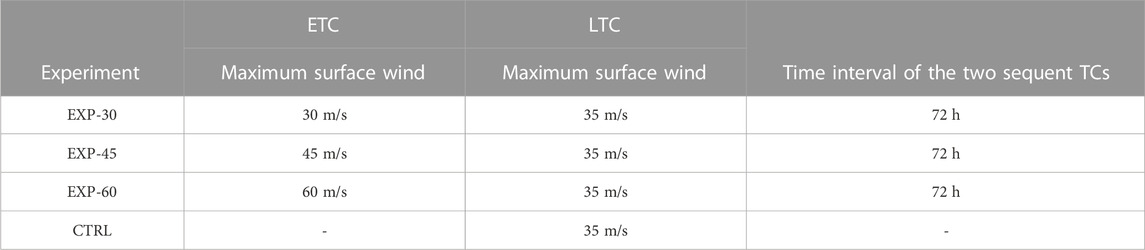
TABLE 1. Sensitivity experiments for the sequential TCs. The wind filed for the, ETC., and LTC are constructed based on the SLOSH method, with a moving speed of 6 m/s and a maximum winds radius of 50 km.
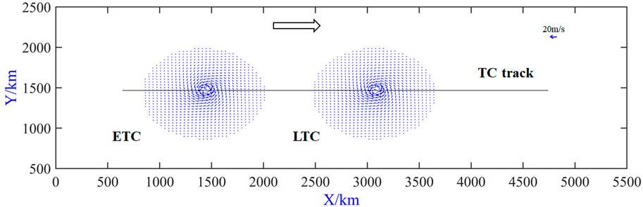
FIGURE 7. The schematics of simulations for sequential TCs.
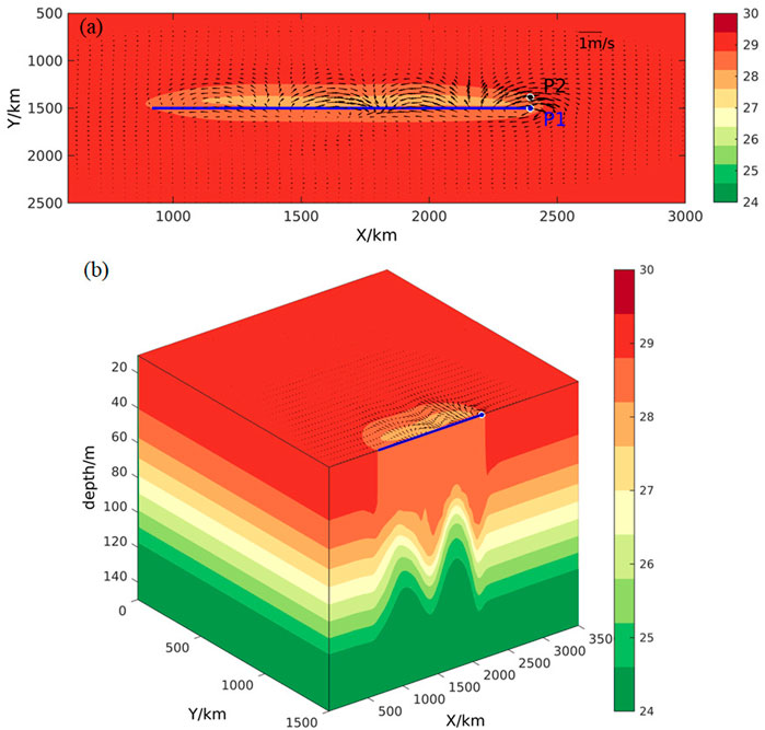
FIGURE 8. (A) Model simulated temperature and velocity at the sea surface and (B) vertical sections on day 3 in the CTRL experiment. In subgraph (A), the roundness label of two selected points is at the center (P1) and 50 km on the right side (P2) of the TC track.
In this study, two points were selected to explore the SST responses to TCs in the four idealized experiments (Figure 8A): one point was the center of the TC track (point 1: P1), and the second was located at 50 km to the right side of the track (point 2: P2). The P2 had an SST cooling of −1.1 °C in the CTRL experiment, compared to −2.21 °C in the EXP-30 experiment, −2.51°C in the EXP-45 experiment, and −3.53 °C in the EXP-60 experiment (Figure 9). It is also clear that the SST cooling at P1 and P2 in the sensitivity experiments are larger than those in the control experiment, consistent with the statistical result reflected in (Figures 3, 5C). Notably, the SST cooling caused by the sequential TCs at P1 and P2 yields an overall increasing trend with a more intense, ETC. The stronger wind stress associated with a more intense, ETC., can produce more significant SST cooling and can contribute more to the SST cooling during the passage of sequential TCs.
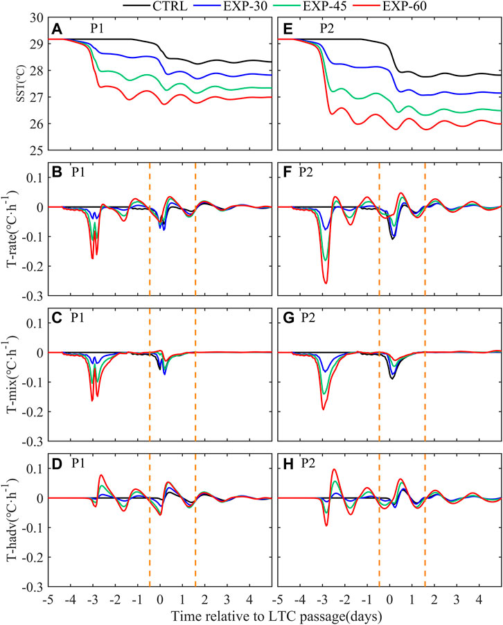
FIGURE 9. The temporal evolutions for the sea surface temperature, local tendency of SST (T-rate), the vertical mixing (T-mix), and the horizontal advection (T-hadv) at P1 and P2 in the CTRL, EXP-30, EXP-45 and EXP-60 experiments. Day 0 refers to the day of the LTC arrival on the local position. The black, blue, gray, and red lines label the different idealized experiments. The orange dashed lines donate the periods during which the contributions of each term in Equation 3 to the LTC-induced SST cooling are calculated.
As shown in Figure 9, each individual term in the surface heat budget analysis at the two selected points further revealed the inhibiting role of the ETC-induced cold wake on the LTC-induced SST cooling. The LTC-induced SST cooling at the P2 (P1) is −0.68°C, −0.67°C, −0.57°C, and −0.44°C (−1.08°C, −0.87°C, −0.65°C, and −0.53°C) in the CTRL, EXP-30, EXP-45, and EXP-60 experiment, respectively (Table 2). The LTC-induced SST cooling showed an overall decreasing trend with the enhancement of the ETC-induced cold wake, consistent with the statistical result of Figure 5B. In the CTRL experiment, the SST change trend kept pace with the change of the vertical mixing at P1 and P2 during the LTC passage. The vertical mixing contributed more than 80% to the maximum SST cooling at both P1 and P2 (Table 2). Previous studies generally suggested that vertical mixing could dominate the total TC-induced SST cooling (Price, 1981; Jullien et al., 2012), which was consistent with the result in the CTRL experiment. At P1 in the EXP-45 experiments, the LTC-induced SST cooling due to vertical mixing is reduced by 80%, compared with that in the CTRL experiment (Table 2). Similarly, for the corresponding experiments, the contribution of vertical mixing at P2 to the SST cooling decreased to 76% of the SST cooling. Especially in the EXP-60 experiment, the SST cooling induced by the vertical mixing had fallen to below 60%. Since a thick mixed layer can effectively restrain the entrainment of cold water (Lin et al., 2008), the LTC-induced SST cooling decreased in the presence of a deepening mixed layer. In the sensitivity experiments, the deepening of the mixed layer by the, ETC., is more profound than that in the CTRL experiment (Figure 12). As a result, during the LTC passage, the SST cooling caused by the vertical mixing in the EXP-60 experiments is smaller than in other experiments, which can be explained by the fact that the corresponding mixed layer is deeper.
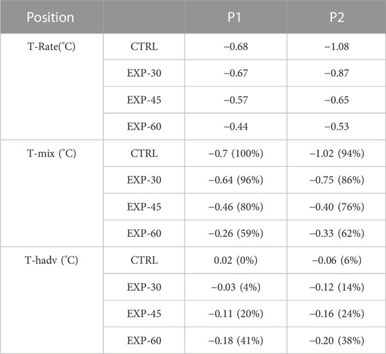
TABLE 2. The changes in SST (°C) and those due to the vertical mixing (T-mix) and the horizontal advection (T-hadv) at the two selected points. The periods for calculating the changes are labeled in Figure 9 with the dashed lines.
However, the contribution of horizontal advection to LTC-induced SST cooling showed an increasing trend with a more intense, ETC. In the EXP-45 experiment, the contribution from horizontal advection (−0.16°C and −0.11 °C at P2 and P1) to the LTC-induced SST cooling was larger than those (0.02°C and −0.06°C at P2 and P1) toin the CTRL experiment (Figure 9; Table 2). In the EXP-60 experiment, the horizontal advection largely accounted for the LTC-induced SST cooling, producing −0.18 (41%) and −0.20 (38%) at P1 and P2, respectively. This result differed from the conclusions of previous studies on single TCs (Price, 1981; Jacob et al., 2000; Jullien et al., 2012). During the passage of sequential TCs, the, ETC., produced asymmetrical SST cooling, and the colder water appeared on the right side of the TC track. Owing to the surface wind stress of the LTC, the colder water on the right side of the TC track rapidly shifted leftward about 1 day before the LTC passage. The horizontal cold advection associated with the cross-track currents was acting to promote the local SST cooling in the presence of the ETC-induced cold wake (Figure 10). As a result, the SST cooling induced by the horizontal cold advection was significantly enhanced during the LTC passage. Similarly, the, ETC., amplified the subsequent horizontal warm advection (Figures 9D, H). The thick mixed layer induced by the, ETC., was acting to prevent local SST cooling by weakening vertical mixing so that more warm water was carried to the left by the surface wind at the half-rear side of the LTC. Overall, horizontal advection contributed to the LTC-induced SST cooling, which was larger with intense, ETCs. During the passage of sequential TCs, the cold wake left behind by the, ETC., led to relatively colder water on the right side of the TC track, which increased the contribution of the horizontal advection to the SST cooling (Figure 10).
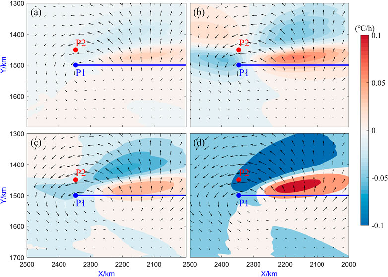
FIGURE 10. The change rate of the SST due to the horizontal advection (°C/h, shaded) at 0 days relative to the LTC passage in the (A) CTRL, (B) EXP-30, (C) EXP-45, and (D) EXP-60 experiment. The black vectors are the currents (m/s, vectors). The blue and red points label points P1 and P2.
To explore the sub-surface thermodynamic changes induced by sequential TCs, P1 was selected as the typical point to investigate the sub-surface temperature response to the sequential TCs. The temperature evolution indicated that the apparent warm and cold water alternately appeared at the sub-surface ocean (Figure 11), which was consistent with the observed result during the TC passage (Li et al., 2022). The mixed layer depth was calculated according to the temperature and salinity from the model results. As shown in Figure 12, The mixed layer depth induced by sequential TCs was deeper than that under the single-TC condition, which is consistent with the results of Figure 6.
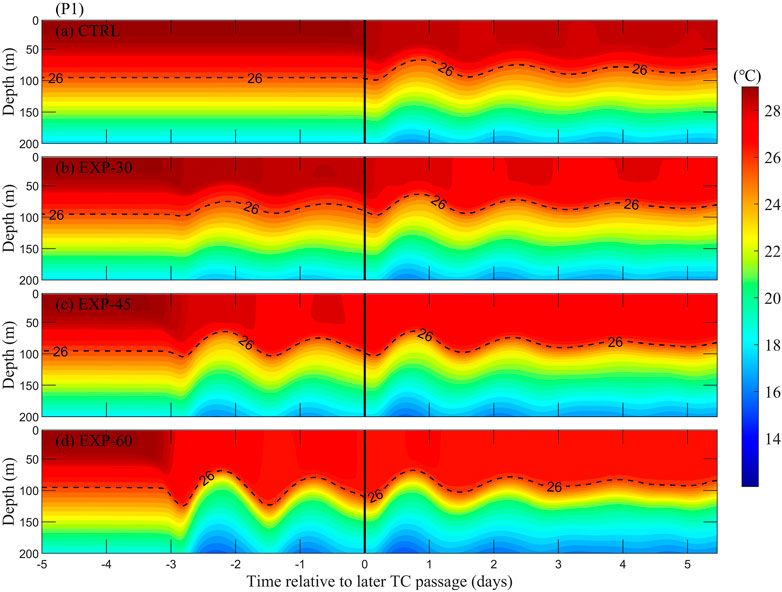
FIGURE 11. Time-depth cross-section of temperature (°C) at point P1 in different experiments. Day 0 is the arrival time of the LTC.
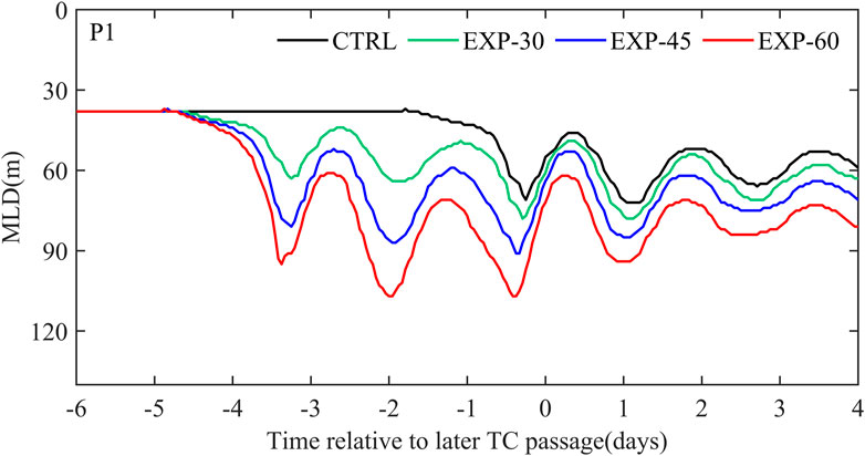
FIGURE 12. The temporal evolution of the MLD (m) during TC passage, day 0 refers to the day of the LTC arrival on the local position. The differently colored solid lines indicate different idealized model experiments.
Figure 13 shows the contributions to the temperature change by vertical mixing, vertical advection, and horizontal advection at P1. Vertical mixing can deepen the mixed layer by warming the sub-surface water temperature, while vertical advection renders the mixed layer to become shallower by cooling the sub-surface water (Zhang et al., 2016). There was a depth difference in the warm temperature anomaly induced by the vertical mixing among the different experiments (Figures 13a1–d1) due to the difference in ETC-induced mixed layer depth. The amplitude of the warm temperature anomalies induced by the vertical mixing was larger in the CTRL experiment than these in the other sensitivity experiments. However, the LTC produced larger vertical advection following a more intense, ETC. Therefore, the joint influence of the weakened vertical mixing and intense vertical advection can suppress the deepening of mixed layer. Even in the EXP-60 experiment, the mixed layer became significantly shallower after the passage of an LTC. As for the horizontal advection, its contribution to the upper ocean thermal response was generally small as compared to that of mixing and upwelling, possibly because most of the flow whirled within the cold wake of a TC. As the surface winds of an, ETC., increased, the effect of the advection showed an overall intensifying trend, while the effect of vertical mixing showed a weakening trend.
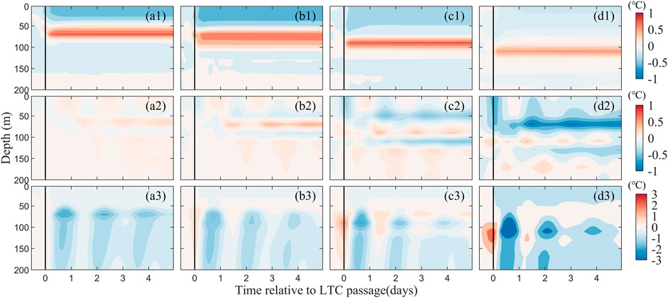
FIGURE 13. Temperature changes caused by the vertical mixing (a1–d1), horizontal advection (a2–d2), and vertical advection (a3–d3) at point P1 in the four experiments. Day 0 is the arrival time of the LTC.
The upper ocean response to sequential TCs was investigated using the 19-year observational datasets (satellite-derived high-resolution SST maps, TC best track data and Argo data) and the heat budget analysis of idealized numerical simulations. Compared to a single TC, the sequential TCs can induce greater surface cooling. However, the SST cooling produced by the LTC of sequential TCs is statistically weaker than that induced by a single TC. Meanwhile, the LTC-induced SST cooling is also modulated by the cold wake left behind by an, ETC. The numerical simulation results revealed that the contribution from horizontal advection to sea surface cooling could be observed even larger than that induced by the vertical mixing during an LTC passage. An, ETC., contributed to a thicker mixed layer thus, restraining the contributions of vertical mixing to SST cooling. On the other hand, an, ETC., produced relative colder water on the right side of the TC track. Before the arrival of an LTC, the relatively colder water was driven by its surfac wind, and propagate leftward. This interaction favors an enhancement of the horizontal cold advection. For the SST cooling, the induced increase by the cross-track horizontal advection can offset the partial reduction caused by vertical mixing. With an intensified, ETC, the horizontal advection contributed to a stronger LTC-induced SST cooling, while the effect of the vertical mixing was weakened. In addition, the more pronounced deepening of mixed layer was observed during the passage of sequential TCs. Compared with a single TC, the influence of an LTC upon the deepening of the mixed layer is weaker.
This study is concerned about cyclone-wake interaction. Based on satellite-derived high-resolution SST maps and idealized numerical simulations, this study emphasized the effect of ETC-induced cold wake on the upper ocean response to a subsequent LTC through regulating advection and vertical mixing.
The original contributions presented in the study are included in the article/Supplementary Material, further inquiries can be directed to the corresponding author.
SH and XC contributed to conception and design of the study, SH wrote the first draft of the manuscript. All authors contributed to manuscript revision, read, and approved the submitted version.
This research was funded by the National Natural Science Foundation of China (42192552).
The authors declare that the research was conducted in the absence of any commercial or financial relationships that could be construed as a potential conflict of interest.
All claims expressed in this article are solely those of the authors and do not necessarily represent those of their affiliated organizations, or those of the publisher, the editors and the reviewers. Any product that may be evaluated in this article, or claim that may be made by its manufacturer, is not guaranteed or endorsed by the publisher.
Balaguru, K., Taraphdar, S., Leung, L. R., Foltz, G. R., and Knaff, J. A. (2014). Cyclone-cyclone interactions through the ocean pathway. Geophys. Res. Lett. 41, 6855–6862. doi:10.1002/2014GL061489
Baranowski, D. B., Flatau, P. J., Chen, S., and Black, P. G. (2014). Upper ocean response to the passage of two sequential typhoons. Ocean Sci. 10 (3), 559–570. doi:10.5194/os-10-559-2014
Chavas, D. R., and Emanuel, K. A. (2010). A QuikSCAT climatology of tropical cyclone size. Geophys. Res. Lett. 37 (18), L18816. doi:10.1029/2010GL044558
Chen, H., Li, S., He, H. L., Song, J. B., Ling, Z., Cao, A. Z., et al. (2020). Obser-vational study of super typhoon Meranti (2016) using satellite, surface drifter. Argo float and reanalysis data. Acta Oceanol. Sin. 40 (1), 70–84. doi:10.1007/s13131-021-1702-9
Chiang, T.-L., Wu, C.-R., and Oey, L.-Y. (2011). Typhoon kai-tak: An ocean's perfect storm. J. Phys. Oceanogr. 41, 221–233. doi:10.1175/2010JPO4518.1
Cione, J. J., Molina, P., Kaplan, J., and Black, P. G. (2000). “SST time series directly under tropical cyclones: Observations and implications,” in 24th conference on hurricanes and tropical meteorology/10th conference on interaction of the sea and atmosphere.
Dare, R. A., and McBride, J. L. (2011). Sea surface temperature response to tropical cyclones. Mon. Weather Rev. 139 (12), 3798–3808. doi:10.1175/MWR-D-10-05019.1
Ezer, T., Arango, H. G., and Shchepetkin, A. F. (2000). Developments in terrain-following ocean models: Intercomparisons of numerical aspects. Ocean. Model. 4, 249–267. doi:10.1016/S1463-5003(02)00003-3
Gelaro, R., McCarty, W., Suárez, M. J., Todling, R., Molod, A., Takacs, L., et al. (2017). The modern-era retrospective analysis for research and applications, version 2 (MERRA-2). J. Clim. 30 (14), 5419–5454. doi:10.1175/JCLI-D-16-0758.1
Girishkumar, M. S., Suprit, K., Chiranjivi, J., Udaya Bhaskar, T. V. S., Ravichandran, M., Shesu, R. V., et al. (2004). Observed oceanic response to tropical cyclone Jal from a moored buoy in the south-Western Bay of Bengal. Ocean. Dyn. 64 (3), 325–335. doi:10.1007/s10236-014-0689-6
He, S., Cheng, X., Fei, J., Wei, Z., Huang, X., and Liu, L. (2022). Thermal response to tropical cyclones over the Kuroshio. Earth Space Sci. 9 (5). doi:10.1029/2021EA002001
Huang, P. S., Sanford, T. B., and Imberger, J. (2009). Heat and turbulent kinetic energy budgets for surface layer cooling induced by the passage of Hurricane Frances (2004). J. Geophys. Res. 114, C12023. doi:10.1029/2009JC005603
Jacob, D. S., Shay, L. K., Mariano, A. J., and Black, P. G. (2000). The 3D oceanic mixed layer response to hurricane gilbert. J. Phys. Oceanogr. 30, 1407–1429. doi:10.1175/1520-0485(2000)030<1407:tomlrt>2.0.co;2
Jaimes, B., and Shay, L. K. (2009). Mixed layer cooling in mesoscale oceanic eddies during Hurricanes Katrina and Rita. Mon. Weather Rev. 137 (12), 4188–4207. doi:10.1175/2009mwr2849.1
Jaimes, B., and Shay, L. K. (2010). Near-inertial wave wake of Hurricanes Katrina and Rita over mesoscale oceanic eddies. J. Phys. Oceanogr. 40 (6), 1320–1337. doi:10.1175/2010JPO4309.1
Jaimes, B., Shay, L. K., and Uhlhorn, E. W. (2015). Enthalpy and momentum fluxes during hurricane earl relative to underlying ocean features. Mon. Weath. Rev. 143 (1), 111–131. doi:10.1175/MWR-D-13-00277.1
Jelesnianski, C. P., and Taylor, A. D. (1973). A preliminary view of storm surges before and after storm modifications. Washington, DC: NOAA Technical Memorandum ERL WMPO-3, 23–33.
Jelesnianski, C. P. (1966). Numerical computation of storm surges without bottom stress, Mon. Weather Rev. 94 (6), 374–379. doi:10.1175/1520-0493(1966)094<0379:NCOSSW>2.3.CO;2
Jeon, C., Watts, D. R., Min, H. S., Kim, D. G., Kang, S. K., Moon, I-J., et al. (2022). Weakening of the Kuroshio upstream by cyclonic cold eddies enhanced by the consecutive passages of typhoons danas, wipha, and francisco (2013). Front. Mar. Sci. 9, 884768. doi:10.3389/fmars.2022.884768
Jullien, S., Marchesiello, P., Menkes, C. E., Lefèvre, J., Jourdain, N. C., Samson, G., et al. (2014). Ocean feedback to tropical cyclones: Climatology and processes. Clim. Dyn. 43, 2831–2854. doi:10.1007/s00382-014-2096-6
Jullien, S., Menkes, C. E., Marchesiello, P., Jourdain, N. C., Lengaigne, M., KochLarrouy, A., et al. (2012). Impact of tropical cyclones on the heat budget of the south Pacific ocean. J. Phys. Oceanogr. 42 (11), 1882–1906. doi:10.1175/jpo-d-11-0133.1
Li, X., Cheng, X., Fei, J., and Huang, X. (2022). A numerical study on the role of mesoscale cold-core eddies in modulating the upper-ocean responses to typhoon trami (2018). J. Phys. Oceanogr. 52 (12), 3101–3122. doi:10.1175/JPO-D-22-0080.1
Lin, I. I., Liu, W. T., Wu, C. C., Wong, G. T. F., Hu, C. M., Chen, Z. Q., et al. (2003). New evidence for enhanced ocean primary production triggered by tropical cyclone. Geophys. Res. Lett. 30 (13), 51. doi:10.1029/2003GL017141
Lin, I. I., Pun, I. F., and Wu, C. C. (2009). Upper-ocean thermal structure and the Western North Pacific category 5 typhoons. Part II: Dependence on translation speed. Mon. Weather Rev. 137 (11), 3744–3757. doi:10.1175/2009MWR2713.1
Lin, I. I., Wu, C. C., Emanuel, K. A., Lee, I.-H., Wu, C. R., and Pun, I. F. (2005). The interaction of Supertyphoon Maemi (2003) with a warm ocean eddy. Mon. Weather Rev. 33 (9), 2635–2649. doi:10.1175/MWR3005.1
Lin, I. I., Wu, C. C., Pun, I. F., and Ko, D. S. (2008). Upper-Ocean thermal structure and the Western North Pacific category 5 typhoons. Part I: Ocean features and the category 5 typhoons’ intensification. Mon. Weather Rev. 136 (9), 3288–3306. doi:10.1175/2008MWR2277.1
Lin, S., Zhang, W. Z., Shang, S. P., and Hong, H. S. (2017). Ocean response to typhoons in the Western North Pacific: Composite results from Argo data. Deep-Sea Res. Part I 123, 62–74. doi:10.1016/j.dsr.2017.03.007
Liu, X., and Wei, J. (2015). Understanding surface and subsurface temperature changes induced by tropical cyclones in the Kuroshio. Ocean. Dyn. 65 (7), 1017–1027. doi:10.1007/s10236-015-0851-9
Liu, X., Zhang, D. L., and Guan, J. (2019). Parameterizing Sea surface temperature cooling induced by tropical cyclones: 2. Verification by ocean drifters. J. Geophys. Res. Oceans 124, 1232–1243. doi:10.1029/2018jc014118
Lloyd, I. D., and Vecchi, G. A. (2010). Observational evidence for oceanic controls on hurricane intensity. J. Clim. 24 (4), 1138–1153. doi:10.1175/2010JCLI3763.1
Ma, Z. H., Fei, J. F., Huang, X. G., and Cheng, X. P. (2018). Modulating effects of mesoscale oceanic eddies on sea surface temperature response to tropical cyclones over the Western North Pacific. J. Geophys. Res. Atmos. 123 (1), 367–379. doi:10.1002/2017JD027806
Ma, Z. H., Fei, J. F., Lei, L., Huang, X. G., and Li, Y. (2017). An Investigation of the influences of mesoscale ocean eddies on tropical cyclone intensities. Mon. Weather Rev. 145 (4), 1181–1201. doi:10.1175/MWR-D-16-0253.1
Mei, W., and Pasquero, C. (2013). Spatial and temporal characterization of sea surface temperature response to tropical cyclones. J. Clim. 26 (11), 3745–3765. doi:10.1175/JCLI-D-12-00125.1
Niwa, Y., and Hibiya, T. (1997). Nonlinear processes of energy transfer from traveling hurricanes to the deep ocean internal wave field. J. Geophys. Res. 102 (C6), 12469–12477. doi:10.1029/97JC00588
Price, J. F., Morzel, J., and Niiler, P. P. (2008). Warming of SST in the cool wake of a moving hurricane. J. Geophys. Res. 113 (C7), C07010. doi:10.1029/2007JC004393
Price, J. F., Sanford, T. B., and Forristall, G. Z. (1994). Forced stage responseto a moving hurricane. J. Phys. Oceanogr. 24, 233–260. doi:10.1175/1520-0485(1994)024<0233:fsrtam>2.0.co;2
Price, J. F. (1981). Upper ocean response to a hurricane. J. Phys. Oceanogr. 11 (2), 153–175. doi:10.1175/1520-0485(1981)011<0153:uortah>2.0.co;2
Samson, G., Giordani, H., Caniaux, G., and Roux, F. (2009). Numerical investigation of an oceanic resonant regime induced by hurricane winds. Ocean. Dyn. 59, 565–586. doi:10.1007/s10236-009-0203-8
Shay, L. K., Goni, G. J., and Black, P. G. (2000). Effects of a warm oceanic feature on Hurricane Opal. Mon. Weather Rev. 128 (5), 1366–1383. doi:10.1175/1520-0493(2000)128<1366:EOAWOF>2.0.CO;2
Thompson, C., Barthe, C., Bielli, S., Tulet, P., Pianezze, J., and Kieu, C. (2021). Projected characteristic changes of a typical tropical cyclone under climate change in the south west Indian ocean. Atmosphere 12 (2), 232. doi:10.3390/atmos12020232
Uhlhorn, E. W., and Shay, L. K. (2013). Loop current mixed layer energy response to Hurricane Lili (2002). Part II: Idealized numerical simulations. J. Phys. Oceanogr. 43 (6), 1173–1192. doi:10.1175/JPO-D-12-0203.1
Vianna, M. L., Menezes, V. V., Pezza, A. B., and Simmonds, I. (2010). Interactions between hurricane catarina (2004) and warm core rings in the south atlantic ocean. J. Geophys. Res. 115 (C7), C07002. doi:10.1029/2009JC005974
Walker, N. D., Leben, R. R., and Balasubramanian, S. (2005). Hurricane-forced upwelling and chlorophyll a enhancement within cold-core cyclones in the Gulf of Mexico. Geophys. Res. Lett. 32, L18610. doi:10.1029/2005GL023716
Walker, N. D., Leben, R. R., Pilley, C. T., Shannon, M., Herndon, D. C., Pun, I. F., et al. (2014). Slow translation speed causes rapid collapse of northeast Pacific Hurricane Kenneth over cold core eddy. Geophys. Res. Lett. 41 (21), 7595–7601. doi:10.1002/2014GL061584
Wang, G., Wu, L., Johnson, N. C., and Ling, Z. (2016). Observed three-dimensional structure of ocean cooling induced by Pacific tropical cyclones. Geophys Res. Lett. 43, 7632–7638. doi:10.1002/2016GL069605
Warner, J. C., Sherwood, C. R., Arango, H. G., and Signell, R. P. (2005). Performance of four turbulence closure models implemented using a generic length scale method. Ocean. Model 8, 81–113. doi:10.1016/j.ocemod.2003.12.003
Wei, J., Liu, X., and Wang, D. X. (2014). Dynamic and thermal responses of the Kuroshio to typhoon Megi (2004). Geophys. Res. Lett. 41, 8495–8502. doi:10.1002/2014gl061706
Wu, C. R., Chang, Y. L., Oey, L. Y., and Hsin, Y. C. (2008). Air-sea interaction between tropical cyclone Nari and Kuroshio. Geophys. Res. Lett. 35 (12). doi:10.1029/2008GL033942
Wu, R., and Li, C. (2018). Upper ocean response to the passage of two sequential typhoons. Deep Sea Res. Part I Oceanogr. Res. Pap. 132, 68–79. doi:10.1016/j.dsr.2017.12.006
Yang, B., Hou, Y., Hu, P., Liu, Z., and Liu, Y. (2015). Shallow ocean response to tropical cyclones observed on the continental shelf of the Northwestern South China sea. J. Geophys Res. Oceans 120, 3817–3836. doi:10.1002/2015JC010783
Ye, H., Sheng, J., Tang, D., Morozov, E., Kalhoro, M. A., Wang, S., et al. (2019). Examining the impact of tropical cyclones on air-sea CO2 exchanges in the Bay of Bengal based on satellite data and in situ observations. J. Geophys. Res. Oceans 124 (1), 555–576. doi:10.1029/2018jc014533
Zhang, H., Chen, D. K., Zhou, L., Liu, X. H., Ding, T., and Zhou, B. F. (2016). Upper ocean response to typhoon Kalmaegi (2014). J. Geophys. Res. Oceans 121 (8), 6520–6535. doi:10.1002/2016JC012064
Zhang, H., Liu, X., Wu, R., Chen, D., Zhang, W., Shang, X., et al. (2020). Sea surface current response patterns to tropical cyclones. J. Mar. Syst. 208, 103345. doi:10.1016/j.jmarsys.2020.103345
Zhang, H., Liu, X., Wu, R., Liu, F., Yu, L., Shang, X., et al. (2019). Ocean response to successive typhoons Sarika and Haima (2016) based on data acquired via multiple satellites and moored array. Remote Sens. 11 (20), 2360. doi:10.3390/rs11202360
Keywords: sequential tropical cyclones, sea surface temperature cooling, mixed layer, idealized numerical experiment, vertical mixing, horizontal advection
Citation: He S, Cheng X, Fei J, Li X, Wei Z and Huang X (2023) Thermal response to sequential tropical cyclone passages: Statistic analysis and idealized experiments. Front. Earth Sci. 11:1142537. doi: 10.3389/feart.2023.1142537
Received: 11 January 2023; Accepted: 28 February 2023;
Published: 13 March 2023.
Edited by:
Jianqi Sun, Institute of Atmospheric Physics (CAS), ChinaReviewed by:
Qing Yan, Institute of Atmospheric Physics (CAS), ChinaCopyright © 2023 He, Cheng, Fei, Li, Wei and Huang. This is an open-access article distributed under the terms of the Creative Commons Attribution License (CC BY). The use, distribution or reproduction in other forums is permitted, provided the original author(s) and the copyright owner(s) are credited and that the original publication in this journal is cited, in accordance with accepted academic practice. No use, distribution or reproduction is permitted which does not comply with these terms.
*Correspondence: Xiaoping Cheng, Y2hlbmd4aWFvcGluZzE3QG51ZHQuZWR1LmNu
Disclaimer: All claims expressed in this article are solely those of the authors and do not necessarily represent those of their affiliated organizations, or those of the publisher, the editors and the reviewers. Any product that may be evaluated in this article or claim that may be made by its manufacturer is not guaranteed or endorsed by the publisher.
Research integrity at Frontiers
Learn more about the work of our research integrity team to safeguard the quality of each article we publish.