 Chunlin Zhang
 Liyong Fan2
 Guiting Chen
95% of researchers rate our articles as excellent or good
Learn more about the work of our research integrity team to safeguard the quality of each article we publish.
Find out more
ORIGINAL RESEARCH article
Front. Earth Sci. , 13 March 2023
Sec. Environmental Informatics and Remote Sensing
Volume 11 - 2023 | https://doi.org/10.3389/feart.2023.1141220
This article is part of the Research Topic Advances and Applications of Artificial Intelligence in Geoscience and Remote Sensing View all 14 articles
Staggered-grid finite-difference (FD) method is widely used to solve the wave equation for the numerical seismic modeling, and it is a key step of the advanced seismic imaging and inversion problem. However, the conventional FD method is prone to instability and dispersion error due to the insufficient approximation accuracy. In this work, we propose an efficient temporal high-order finite-difference (FD) scheme with the cross-rhombus stencil. Compared with the standard cross-rhombus method, the new method has less computational cost due to we simplify the FD scheme. Moreover, the dispersion relation of the new method is easy to obtain the dispersion-relation-preserving (DRP) FD coefficients, which can significantly alleviate the spatial and temporal dispersion errors. Dispersion and stability analyses indicate that the new scheme has better performance in seismic modeling than the conventional method, and numerical experiments also indicate that the new scheme can effectively mitigate dispersion error and improve the numerical accuracy.
Staggered-grid finite-difference methods have been extensively applied in the seismic wave simulations due to their straightforward implementation and high computing efficiency (Kindelan et al., 1990; Moczo et al., 2000; Etgen and O¡¯Brien, 2007; Moczo et al., 2011; Moczo et al., 2014; Etemadsaeed et al., 2016; Liu et al., 2019; Zhang et al., 2022). High-order approximation for temporal derivatives in the staggered-grid FD scheme contributes to suppressing the temporal dispersion errors, and enhancing the stability with a large time step. However, the explicit high-order temporal derivative approximation in the FD scheme is always unstable (Chen, 2007; 2011). Generally, we use a second-order temporal approximation and an arbitrary even-order spatial approximation to solve the scalar wave equation.
To improve the temporal accuracy, Dablain (1986) proposed a new FD scheme based on the Lax-Wendroff approach, which can reach fourth-order accuracy in the temporal derivative approximation but has a limitation in the case of the large velocity contrast. Chen (2007, 2011) further developed the fourth- and sixth-order schemes and analyzed the stability condition in the high-order cases. Alternatively, Liu and Sen (2009) proposed the time-space domain FD coefficients by incorporating the dispersion relation of the temporal and spatial terms. The time-space domain method can reach arbitrary even-order accuracy along with some specific propagation angles. However, it is still second-order accuracy along with other angles (Liu and Sen, 2009). To further improve the accuracy, Liu and Sen (2013) proposed a novel rhombus stencil. This new stencil with the time-space domain FD coefficients can reach arbitrary-order accuracy in both temporal and spatial approximations. However, the standard rhombus stencil is not a computationally friendly method for large-scale modeling, and it will increase the computational cost exponentially for the high-order cases. Afterwards, Tan and Huang (2014a),Tan and Huang (2014b) proposed an effective FD stencil with the sixth-order accuracy in the time approximation. Tan’s stencil is similar to the rhombus stencil, but it involves fewer grid nodes outside the cross axis compared to the standard rhombus stencil, thus reducing the computational cost significantly. Wang E. et al. (2016) generally defined this stencil as the cross-rhombus stencil with arbitrary even-order temporal accuracy. The cross-rhombus stencil contains a large cross stencil and a small rhombus stencil. Among them, the small rhombus stencil increases the temporal accuracy and ensures computational efficiency, while the large cross stencil has a high-order spatial accuracy. Then, Ren et al. (2017) developed the cross-rhombus stencil in the staggered-grid FD scheme, and presented two methods for solving the FD coefficients. Wang et al. (2019) further developed the cross-rhombus stencil in the 3D case with the general cuboid grid.
To mitigate the dispersion error, the dispersion relation of the FD scheme should require many wavenumbers, because the spatial dispersion error usually comes from the high-wavenumber component. However, the conventional Taylor series expansion (TE) method for solving FD coefficient satisfies the dispersion relation near the zero wavenumbers, so it is prone to dispersion. The optimization method is a feasible way to obtain the FD coefficients (Liu, 2013; Zhang and Yao, 2013; Tan and Huang, 2014b; Chen et al., 2020) for mitigating dispersion, where the dispersion-relation-preserving method (Wang and Teixeira, 2003; Ye and Chu, 2005; Liang et al., 2015; Etemadsaeed et al., 2016; Chen et al., 2020) has been widely concerned because of its simplicity and easy implementation. The DRP-based method expands dispersion relation into an over-determined system associated with a series of wavenumbers and propagation angles, and then solves this over-determined system numerically to obtain the FD coefficients in the least square sense. The DRP-based FD coefficients satisfy a series of wavenumbers from low to high in the sense of the least square, thus the DRP-based method can effectively mitigate the temporal and spatial dispersion error.
The DRP-based FD coefficients have been successfully applied to the temporal high-order scheme (cross-rhombus stencil) in the regular grid Chen et al. (2020), in which the DRP-based coefficients can significantly mitigate dispersion error, while the cross-rhombus stencil can effectively improve the temporal approximation accuracy. However, for the staggered-grid FD scheme, the DRP-based coefficients cannot be directly obtained because the dispersion relation is difficult to be extended into an over-determined system. Liang et al. (2018) has presented a special FD scheme with a high computational efficiency, in which the second-order FD operator is used to approximate some partial derivatives rather than the global high-order FD operator. And such replacement simplifies the dispersion relation into a form of the linear equation. Motivated by (Liang et al., 2018; Zhou et al., 2022), we propose a general simplified FD scheme for the temporal high-order modeling with a cross-rhombus stencil. The new scheme contains a cross stencil with the analytic FD coefficients and a cross-rhombus stencil with the DRP-based coefficients for different partial derivatives. The cross stencil can simplify the dispersion relation, which makes it easy to construct the over-determined system. The cross-rhombus stencil can make the FD scheme maintain a high-order temporal approximation. The dispersion relation of our new FD scheme can be expanded to an over-determined system with a series of wavenumbers and angles. Solving this over-determined system by the numerical methods (Wang et al., 2014; Wang et al., 2016 Y.; Chen et al., 2020; Wu et al., 2020; Li et al., 2022), we obtain the DRP-based FD coefficients. Therefore, the new FD scheme has three advantages: 1. The DRP-based FD coefficients can effectively mitigate the dispersion error; 2. It still has a temporal higher-order approximation accuracy; 3. The computational cost of the proposed method is significantly reduced compared with the standard cross-rhombus scheme.
The 2D first-order acoustic wave equations with the constant density are
where K = ρυ2 is the bulk modulus, ρ(x, z) is the density and v(x, z) is the velocity. p(x, z, t) is the pressure, and
Here,
and
The superscript CR represents the cross-rhombus stencil composed of a standard cross stencil and a rhombus stencil (as shown in Figure 1). am,n and bm,n represent the FD coefficients of the operators
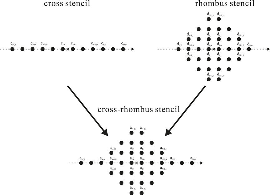
FIGURE 1. Illustrating the cross-rhombus stencil in the staggered grid.
Assuming plane wave propagating in the grid, we let
where kx = k cos(θ) and kz = k sin(θ) are the wavenumbers in x- and z-axes, respectively. θ is a propagation angle of the plane wave, ω is the angular frequency and
Here, r = vτ/h is the Courant number. Generally, the operators HCR and DCR adopt the same FD coefficients, i.e.
Then, Equation 6 can be rewritten as
Eq. 8 represents the time-space domain dispersion relation of the staggered-grid FD scheme with the cross-rhombus stencil. Using the Taylor series to expand the trigonometric functions with respect to the propagation angle θ, we can obtain the time-space domain TE-based FD coefficients (Ren et al., 2017). The cross-rhombus stencil with the TE-based FD coefficients can achieve arbitrary even-order temporal accuracy, thus mitigating the temporal dispersion error significantly.
The TE-based FD coefficients satisfy the dispersion relation within a limited wavenumber bandwidth, resulting in the high-wavenumber components of seismic wavefield are prone to the spatial dispersion. However, the dispersion relation of the standard staggered-grid scheme is a quadratic equation, which is difficult to expand into the over-determined system for solving DRP-based FD coefficients. In this part, we develop a new simplified staggered-grid FD scheme. The new scheme can not only easily obtain the over-determined system for the DRP-based coefficients, but also greatly reduce the computational cost.
The FD operators DCR and HCR use same coefficients (am,n = bm,n), which causes the dispersion relation to be a second-order non-linear equation. To obtain a simple dispersion relation, we propose a new simplified FD scheme as
Here, the superscript C represents the cross stencil. For example, the FD operator
We use the cross-stencil-based operators DC to replace part of the operator DCR in the new scheme. Thus, the new scheme contains a cross-rhombus stencil and a cross stencil for different partial derivatives.
For convenience, DC adopts the analytic time-space domain FD coefficients
Here, L represents the length of the analytic FD operator. And the analytical cross stencil simplifies the original second-order dispersion relation to a linear form. The new dispersion relation can be easily extended to an over-determined linear system for solving the wide-bandwidth FD coefficients. Moreover, the analytical cross stencil has less computational cost compared with the standard cross-rhombus scheme, especially in the high-order cases.
In this part, we present the method for solving the DRP-based FD coefficients of the new scheme. We assume that the plane wave propagating in the grid, and then substitute Eq. 5 into Eq. 9, yield the new dispersion relation
Clearly, the new dispersion relation can be easily extended to the linear system satisfying a series of wavenumbers and propagation angles. It is worth noting that if the FD operator H uses cross stencil, for example: HC and DCR are applied to Equation 9, the dispersion relation does not change. And the cross stencil is applied to the FD operator H or D, the corresponding FD schemes are equivalent.
Following our previous work (Chen et al., 2020), we define a new function ψm,β,θ to represent the weights of FD coefficients am,0 in Eq. 12. Then ψm,β,θ can be denoted as
Here, β = kh and θ represents the propagation angle. Similarly, we define another function χm,n,β,θ to represent the weights of am,n. The function χm,n,β,θ is defined as
Since am,n = an,m, we define a new function
Therefore, the dispersion relation (Eq. 12) of the new FD scheme can be rewritten as
Then we extend ψm,β,θ to a matrix involving a series of β and a fixed angle θ, and the matrix is
Where βi = βmax/ξ*i, βmax = 2πfmax/v with respect to the maximum frequency of the seismic wavefield Chen et al. (2022) and π is the circular constant.
Similarly, we extend the function φn,β,θ to the matrix.
Note that if N is an odd number, the matrix B(θ) is.
The right-hand side of Eq. 16 also be expanded to the matrix
Then the dispersion relation satisfying ξ wavenumbers and ζ angles can be expressed as
This over-determined system has ζ × ξ rows and 1 + M + N2/4 columns with even number N and 1 + M + (N − 1)2/4 columns with odd number N. We can easily obtain the DRP-based FD coefficients by solving this over-determined system. We also introduce the simplified FD scheme in the 3D case, the details are shown in the Supplementary Material S1.
In this part, we analyse the dispersion characteristics of our new scheme. The phase velocity of the new FD scheme can be expressed as
where q is
Thus, the dispersion parameter δ of the new FD scheme is defined as
If δ is not equal to 1, the FD scheme suffers from the numerical dispersion, i.e., has the spatial dispersion error (δ < 1) or temporal dispersion error (δ > 1). We analyze and compare the dispersion parameter δ of the new FD scheme with the other three methods, and the abbreviations of these methods are listed in Table 1. The dispersion curves of δ varying with the kh are shown in Figure 2. It can be seen that the cross-stencil-based FD schemes (TE-C-S and TE-C-TS methods) have obviously temporal dispersion error (δ > 1). The corresponding temporal dispersion of the cross-rhombus stencil (TE-CR-TS and DRP-CR-TS methods) is alleviated (Figures 2C, D) due to the temporal high-order approximation. It is worth noting that the proposed method (DRP-CR-TS method) satisfies the widest range of the wavenumber (kh), which can mitigate the spatial dispersion error considerably.
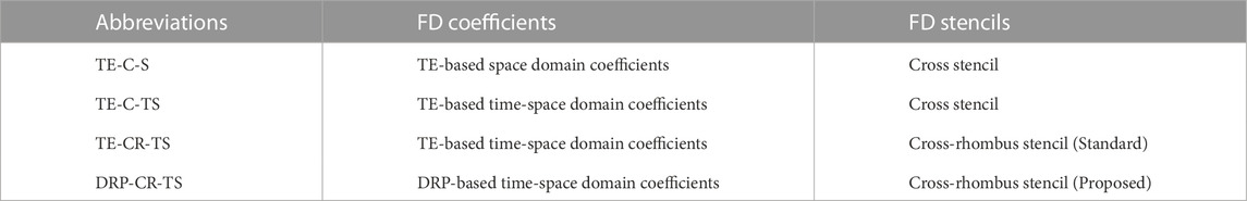
TABLE 1. Abbreviation table of different FD methods used for dispersion analyses.
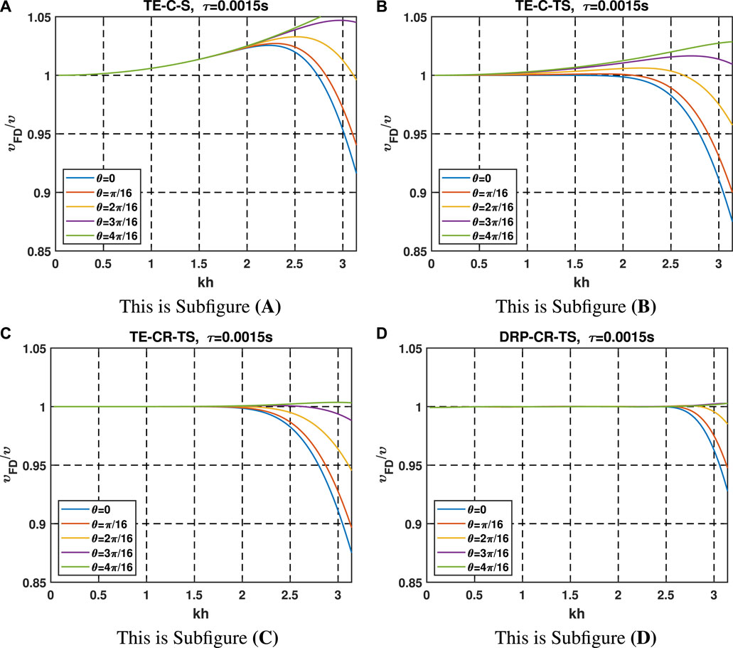
FIGURE 2. Dispersion curves of the four methods with a moderate time step τ=0.0015 s (A) TE-C-S method. (B) TE-C-TS method. (C) TE-CR-TS method. (D) DRP-CR-TS method.
According to the dispersion relation of the new FD scheme, we obtain
It is clear that
Then, we obtain
and
We consider the Nyquist wavenumber, that is
Substituting Eq. 29 into (28), we obtain the stability condition
We denote the right-hand side of inequation (30) as the stability factor
where the stability factor s is related to the FD coefficients am,n and bl,0, and these FD coefficients are determined by the Courant number r. In the following, we analyze the stability factors s varying with the Courant number r, the stability curves of our new scheme and other three methods are shown in Figure 3. It can be seen that the stability factors of the proposed method are slightly less than that of the TE-CR-TS method. Although the DRP-CR-TS method adopts an analytical cross stencil, its stability does not sharp decrease, and it is much larger than that of the conventional methods (TE-C-S and TE-C-TS). Figure 4 shows the maximum value of stability factors satisfying r ≤ s for different orders M. The stability curve of DRP-CR-TS method is volatile due to the use of numerical method to solve the over-determined system, and it is sensitive to order M, but this does not affect the overall stability. It can be seen that the stability curve of the proposed method has the same level with the TE-CR-TS method. Stability analyses in Figures 3, 4 reveals that the proposed scheme has the same level stability as the standard temporal high-order scheme (TE-CR-TS method), and far better than the conventional scheme.
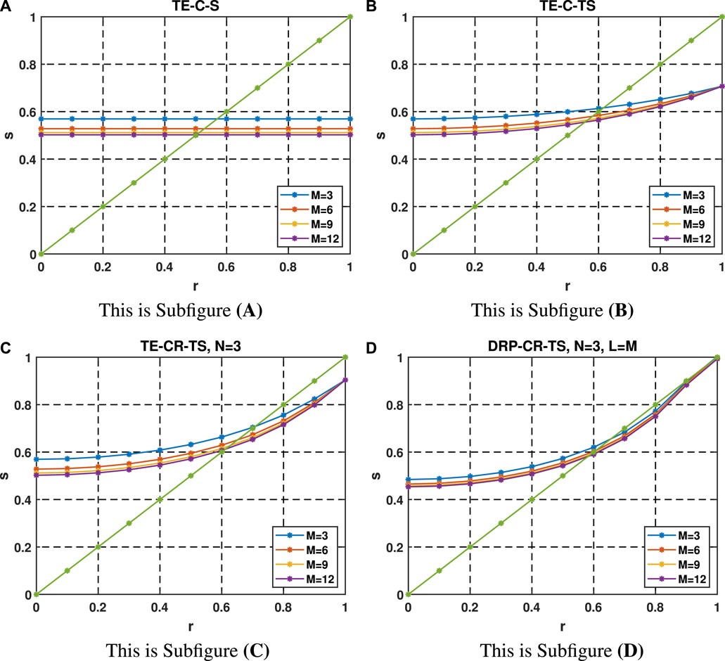
FIGURE 3. Stability factors of the four methods with different r and M, where N =3 and L = M for the cross-rhombus stencil. The green curve represents s(r)= r. (A) TE-C-S method. (B) TE-C-TS method. (C) TE-CR-TS method. (D) DRP-CR-TS method.
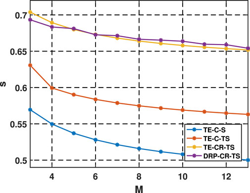
FIGURE 4. Maximum stability factors of the four methods satisfy r ≤ s for different M, where N =3 and L = M for the cross-rhombus stencil.
In this section, we use a 2-D homogeneous velocity model to examine our new scheme. The 2D homogeneous model has 512 × 512 grid nodes with the grid spacing h = 6m and velocity υ = 1500 m/s. A Ricker-wavelet source with a main frequency of 40Hz is located at the spatial point (1536m, 1536m). Two receivers at the spatial points (768m, 768m) and (768m, 1536m) are used to record the waveforms.
Figure 5 shows the snapshots with a time step τ = 0.001s. The TE-C-S and TE-C-TS methods have serious temporal and spatial dispersion errors (Figure 5A). The temporal dispersion error (red arrow) of the TE-CR-TS method is smaller than that of the TE-C-TS method. However, the TE-CR-TS method still has obvious spatial dispersion error (white arrow), because the TE-based FD coefficients preserve the dispersion relation in a limited range. Figure 5D shows that the corresponding spatial dispersion error is reduced considerably in the proposed method (DRP-CR-TS). Figure 6 shows the seismic records of the four methods at Receiver 1 and Receiver 2. The reference traces represented by the green curves are obtained by the high-order FD scheme under the fine grid. The Receiver 1 (Figure 6A) shows that the temporal dispersion errors of the TE-CR-TS and DRP-CR-TS methods are smaller than that of the TE-C-S and TE-C-TS methods, and the Receiver 2 shows that the spatial dispersion error are serious in the TE-based methods (TE-C-S, TE-C-TS, and TE-CR-TS). But the proposed method (DRP-CR-TS) still has a small level of the dispersion error. Table 2 lists the relative errors of the four methods compared to the reference trace at Receiver 1 and Receiver 2. The relative errors of the cross-rhombus stencil are smaller than that of the conventional cross stencil, especially the DRP-CR-TS method reduces the relative error significantly.
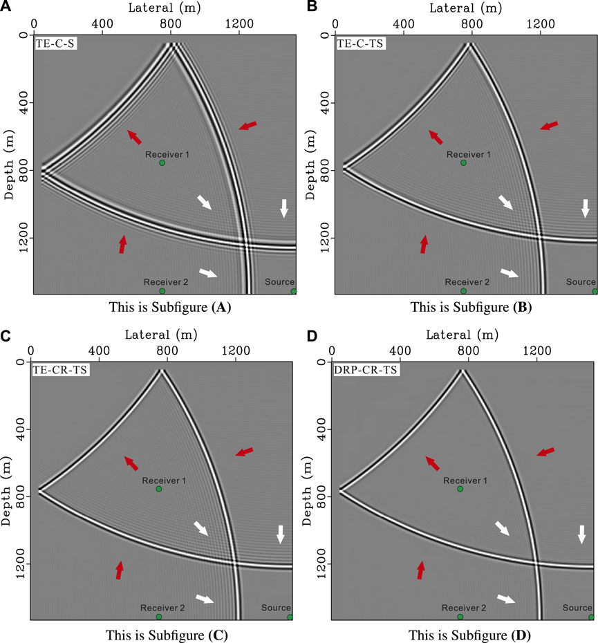
FIGURE 5. Snapshots of the four methods with the time step τ =0.001s, where M =8, N =3, L = M, υ =1500 m/s and h =6m. The main frequency of the Ricker wavelet is 40Hz. (A) TE-C-S method. (B) TE-C-TS method. (C) TE-CR-TS method. (D) DRP-CR-TS method.
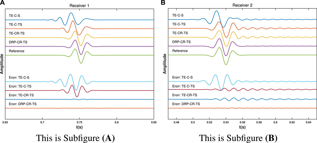
FIGURE 6. Seismic records of the four methods at Receiver 1 and Receiver 2. The reference traces represented by the green curves are obtained by the high-order FD scheme under the fine grid. (A) Seismic records at Receiver 1. (B) Seismic records at Receiver 2.
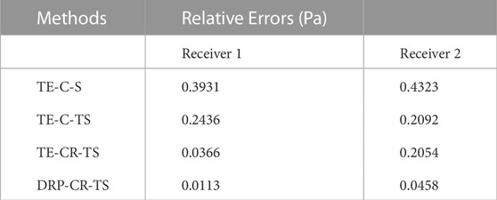
TABLE 2. Relative errors of the four methods at Receiver 1 and Receiver 2.
We also analyze the snapshots for different orders M, the snapshots are shown in Figure 7. In this case, simply increasing M can not effectively reduce the dispersion error in the TE-C-S method. The temporal dispersion errors of the TE-C-TS and TE-CR-TS methods are gradually reduced, but when M = 12, there are still obvious spatial dispersion error (white arrow). The corresponding spatial dispersion error is mitigated in the proposed method (DRP-CR-TS) even at low order (M = 6). Then, we study the snapshots of the proposed method for different N and L, the results are shown in Figure 8. The dispersion error of the proposed method is small for different L and N, thus we can select an appropriate low-order L or N to improve the computational efficiency.
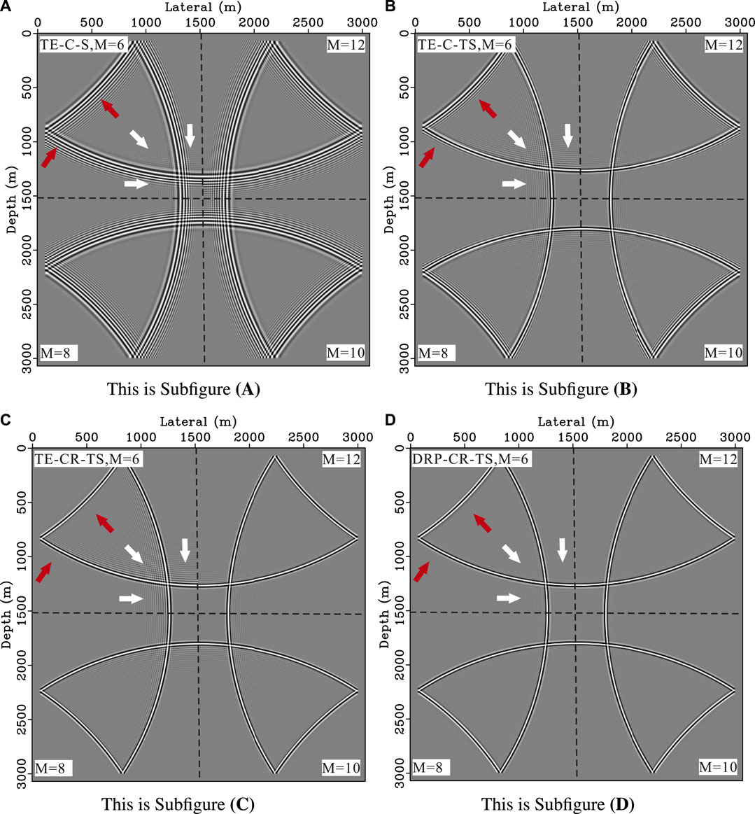
FIGURE 7. Snapshots of the four methods for different M, where τ =0.0015s, υ =1500 m/s, h =6m, and N =3, L = M. The main frequency of the Ricker wavelet is 40Hz. The four quadrants represent the snapshots of the same FD method for different M =6,8,10,12, respectively. (A) TE-C-S method. (B) TE-C-TS method. (C) TE-CR-TS method. (D) DRP-CR-TS method.
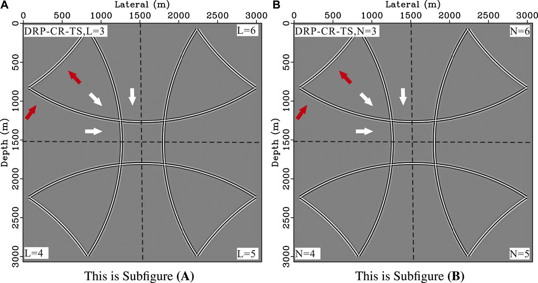
FIGURE 8. Snapshots of the simplified scheme for different L and N, where M =8, τ =0.0015s, υ =1500 m/s and h =6m. The main frequency of the Ricker wavelet is 40Hz. (A) DRP-CR-TS method with different L, here N =3. (B) DRP-CR-TS method with different N, here we set L = M.
We use a widely referred 2D BP velocity model (Figure 9) to test the four methods in the inhomogeneous model. The 2D BP model has 560 × 1000 grid nodes with the variation of velocities from 1500 m/s to 4500 m/s. In this case, we set time step τ = 0.0007 s, M = 8, N = 3, L = M, grid spacing h = 7.5m and main frequency fm = 30Hz for numerical simulation. A total of 1,000 receivers are located on the surface of the model.
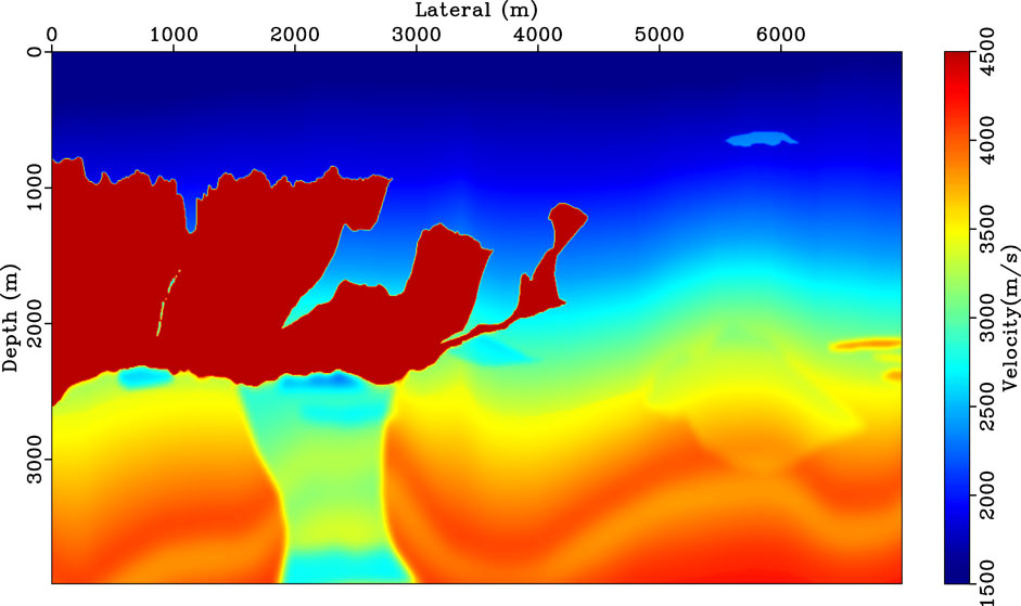
FIGURE 9. BP model with 560×1000 grid nodes and grid spacing h =7.5 m, the variation of velocities from 1500 m/s to 4500 m/s.
Figure 10 shows the snapshots of the four methods. The TE-C-S method has obvious temporal dispersion error (red arrow), and the corresponding error in the TE-C-TS and TE-CR-TS methods is reduced (Figures 10B, C). However, the spatial dispersion error (white arrow) is still serious. Figure 10D shows the spatial dispersion error of the proposed method (DRP-CR-TS) is significantly reduced in the low- and high-velocity layers. Figure 11 shows the seismic records of the four methods, and Figure 12 shows the corresponding seismic records at (1920m, 0m). It can be seen that the TE-based methods have serious spatial dispersion error from the first arrivals, but the corresponding error is mitigated in the proposed method (DRP-CR-TS). The reflected wave from the high-velocity layers contain both the spatial and temporal dispersion errors, and the corresponding error in the proposed method (DRP-CR-TS) is smaller than that of the other three methods.
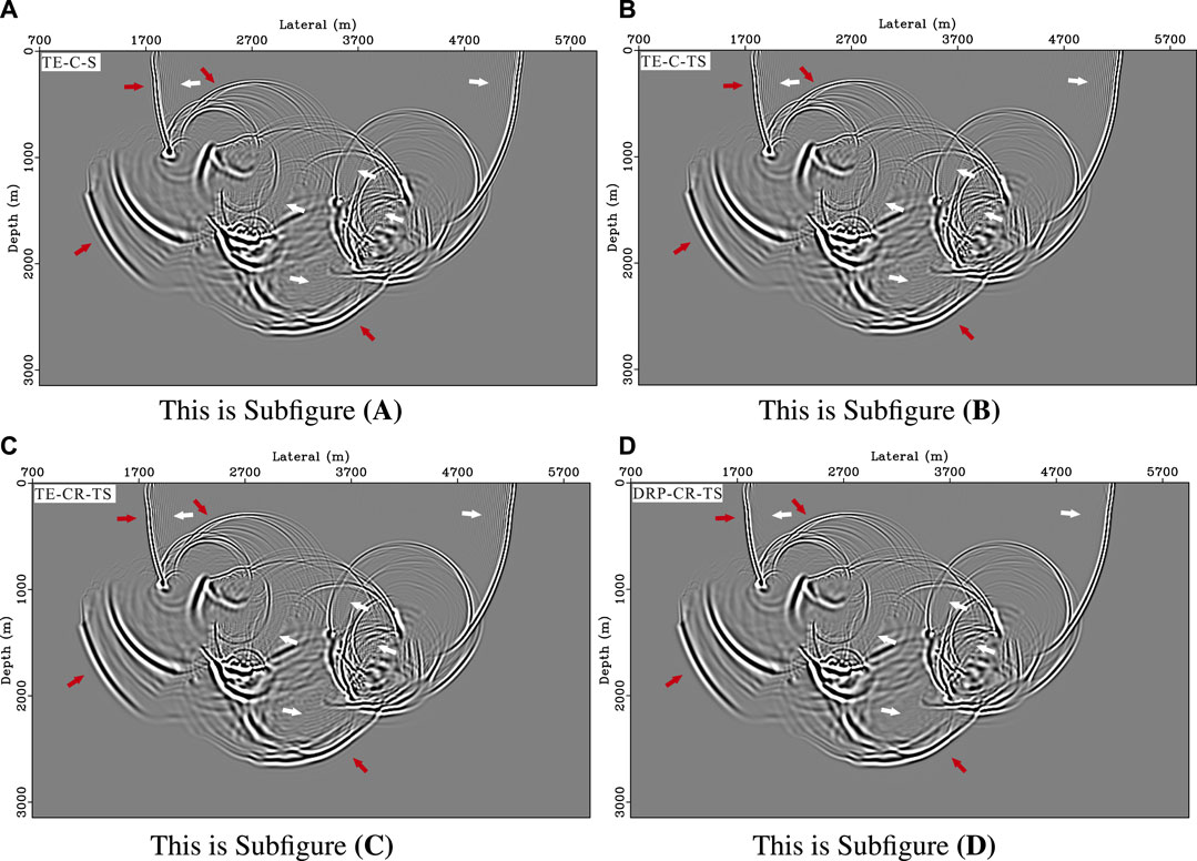
FIGURE 10. Snapshots of the four methods, here we set M =8, N =3, L = M and τ =0.007s (A) TE-C-S method. (B) TE-C-TS method. (C) TE-CR-TS method. (D) DRP-CR-TS method.
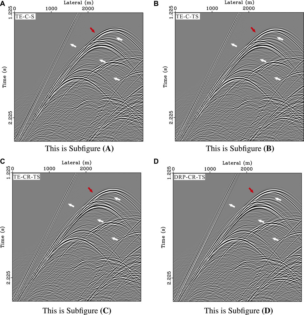
FIGURE 11. Seismic records of the four methods. (A) TE-C-S method. (B) TE-C-TS method. (C) TE-CR-TS method. (D) DRP-CR-TS method.
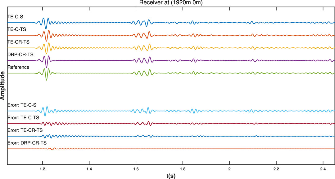
FIGURE 12. Seismic records of the four methods at (1920 m, 0 m).
In this section, we discuss the computational cost and accuracy simultaneously. Taking the above BP model as an example, we design a series of FD parameters for seismic modeling. The numerical experiments are executed on the same computer (Intel Core I7-700 with 3.6 GHz and 8 GB memory). Table 3 shows the CPU execution times and the relative errors at spatial point (1920 m, 0 m) of the four methods. It is clear that the TE-C-S and TE-C-TS methods have fewer execution times in the numerical experiments (Cases 1 and 2 in Table 3), but their relative errors are larger than that of the TE-CR-TS and DRP-CR-TS methods. The relative error of the DRP-CR-TS method is significantly reduced, and their execution time is less than that of the TE-CR-TS method. It is worth noting that when we reduce the length of the analytic FD operator in the DRP-CR-TS method (Cases 5 and 6), the execution time is reduced considerably, and the relative error is almost unaffected. Besides, the DRP-CR-TS method can select a relatively larger time step to reduce the computational cost due to the temporal high-order approximation.
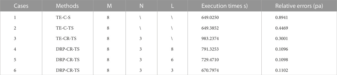
TABLE 3. CPU execution times and the relative errors of the four methods on the BP model.
We propose a new staggered-grid DRP-based FD scheme with a cross-rhombus stencil for solving the scalar wave equation. The new scheme has a simplified dispersion relation, which is convenient for solving the dispersion-relation-preserving FD coefficients. Besides, the simplified scheme uses the cross stencil instead of the cross-rhombus stencil in some FD operators, thus reducing the computational cost considerably. Dispersion analyses reveals that the proposed FD scheme can effectively mitigate the dispersion error, and it still has a temporal higher-order approximation accuracy. The proposed scheme also has better stability compared with the conventional scheme. Numerical experiments show that the proposed scheme has smaller temporal and spatial dispersion errors while ensuring the computational efficiency, and it is an economical way for the large-scale seismic modeling.
The original contributions presented in the study are included in the article/Supplementary Material, further inquiries can be directed to the corresponding authors.
Conceptualization is contributed by CZ and GC; investigation is contributed by CZ, GC, LF, and XZ; data contributed by CZ, GC; formal analysis is contributed by CZ and GC; writing—original draft preparation is contributed by CZ, GC; writing—review and editing is contributed by CZ, LF, and XZ.
This research was funded by the Prospective and Basic Research Project of CNPC (2021DJ0506), Major Technical Project of CNPC (2022KT0302) and China National Science and Technology Major Project (2016ZX05007-002).
This study has benefitted from the reproducible codes and documentation provided in the Madagascar open-source software(Fomel et al., 2013). The authors appreciate the owner of the copyrights.
The authors declare that the research was conducted in the absence of any commercial or financial relationships that could be construed as a potential conflict of interest.
All claims expressed in this article are solely those of the authors and do not necessarily represent those of their affiliated organizations, or those of the publisher, the editors and the reviewers. Any product that may be evaluated in this article, or claim that may be made by its manufacturer, is not guaranteed or endorsed by the publisher.
The Supplementary Material for this article can be found online at: https://www.frontiersin.org/articles/10.3389/feart.2023.1141220/full#supplementary-material
Chen, G., Peng, Z., and Li, Y. (2022). A framework for automatically choosing the optimal parameters of finite-difference scheme in the acoustic wave modeling. Comput. Geosciences 159, 104948. doi:10.1016/j.cageo.2021.104948
Chen, G., Wang, Y., Wang, Z., and Zhang, S. (2020). Dispersion-relationship-preserving seismic modelling using the cross-rhombus stencil with the finite-difference coefficients solved by an over-determined linear system. Geophys. Prospect. 68, 1771–1792. doi:10.1111/1365-2478.12953
Chen, J.-B. (2011). A stability formula for lax-wendroff methods with fourth-order in time and general-order in space for the scalar wave equation. Geophysics 76, T37–T42. doi:10.1190/1.3554626
Chen, J.-B. (2007). High-order time discretizations in seismic modeling. Geophysics 72, SM115–SM122. doi:10.1190/1.2750424
Dablain, M. (1986). The application of high-order differencing to the scalar wave equation. Geophysics 51, 54–66. doi:10.1190/1.1442040
Etemadsaeed, L., Moczo, P., Kristek, J., Ansari, A., and Kristekova, M. (2016). A no-cost improved velocity-stress staggered-grid finite-difference scheme for modelling seismic wave propagation. Geophys. J. Int. 207, 481–511. doi:10.1093/gji/ggw287
Etgen, J. T., and O¡¯Brien, M. J. (2007). Computational methods for large-scale 3d acoustic finite-difference modeling: A tutorial. Geophysics 72, SM223–SM230. doi:10.1190/1.2753753
Fomel, S., Sava, P., Vlad, I., Liu, Y., and Bashkardin, V. (2013). Madagascar: Open-source software project for multidimensional data analysis and reproducible computational experiments. J. Open Res. Softw. 1.
Kindelan, M., Kamel, A., and Sguazzero, P. (1990). On the construction and efficiency of staggered numerical differentiators for the wave equation. Geophysics 55, 107–110. doi:10.1190/1.1442763
Li, S., Yue, B., Chen, Y., Peng, Z., and Wu, R.-S. (2022). Multichannel impedance inversion in the frequency domain via anisotropic total variation with overlapping group sparsity regularization. J. Inverse Ill-posed Problems 30, 307–321. doi:10.1515/jiip-2018-0074
Liang, W., Wang, Y., and Yang, C. (2015). Determining finite difference weights for the acoustic wave equation by a new dispersion-relationship-preserving method. Geophys. Prospect. 63, 11–22. doi:10.1111/1365-2478.12160
Liang, W., Wu, X., Wang, Y., and Yang, C. (2018). A simplified staggered-grid finite-difference scheme and its linear solution for the first-order acoustic wave-equation modeling. J. Comput. Phys. 374, 863–872. doi:10.1016/j.jcp.2018.08.011
Liu, W., He, Y., Li, S., Wu, H., Yang, L., and Peng, Z. (2019). A generalized 17-point scheme based on the directional derivative method for highly accurate finite-difference simulation of the frequency-domain 2d scalar wave equation. J. SEISMIC Explor. 28, 41–71.
Liu, Y. (2013). Globally optimal finite-difference schemes based on least squares. Geophysics 78, T113–T132. doi:10.1190/geo2012-0480.1
Liu, Y., and Sen, M. K. (2009). A new time–space domain high-order finite-difference method for the acoustic wave equation. J. Comput. Phys. 228, 8779–8806. doi:10.1016/j.jcp.2009.08.027
Liu, Y., and Sen, M. K. (2013). Time-space domain dispersion-relation-based finite-difference method with arbitrary even-order accuracy for the 2d acoustic wave equation. J. Comput. Phys. 232, 327–345. doi:10.1016/j.jcp.2012.08.025
Moczo, P., Kristek, J., Galis, M., Chaljub, E., and Etienne, V. (2011). 3-d finite-difference, finite-element, discontinuous-galerkin and spectral-element schemes analysed for their accuracy with respect to p-wave to s-wave speed ratio. Geophys. J. Int. 187, 1645–1667. doi:10.1111/j.1365-246x.2011.05221.x
Moczo, P., Kristek, J., and Galis, M. (2014). The finite-difference modelling of earthquake motions: Waves and ruptures. Cambridge University Press.
Moczo, P., Kristek, J., and Halada, L. (2000). 3d fourth-order staggered-grid finite-difference schemes: Stability and grid dispersion. Bull. Seismol. Soc. Am. 90, 587–603. doi:10.1785/0119990119
Ren, Z., Li, Z., Liu, Y., and Sen, M. K. (2017). Modeling of the acoustic wave equation by staggered-grid finite-difference schemes with high-order temporal and spatial accuracy. Bull. Seismol. Soc. Am. 107, 2160–2182. doi:10.1785/0120170068
Tan, S., and Huang, L. (2014b). A staggered-grid finite-difference scheme optimized in the time–space domain for modeling scalar-wave propagation in geophysical problems. J. Comput. Phys. 276, 613–634. doi:10.1016/j.jcp.2014.07.044
Tan, S., and Huang, L. (2014a). An efficient finite-difference method with high-order accuracy in both time and space domains for modelling scalar-wave propagation. Geophys. J. Int. 197, 1250–1267. doi:10.1093/gji/ggu077
Wang, E., Ba, J., and Liu, Y. (2019). Temporal high-order time–space domain finite-difference methods for modeling 3D acoustic wave equations on general cuboid grids. Pure Appl. Geophys. 176, 5391–5414. doi:10.1007/s00024-019-02277-2
Wang, E., Liu, Y., and Sen, M. K. (2016a). Effective finite-difference modelling methods with 2-d acoustic wave equation using a combination of cross and rhombus stencils. Geophys. J. Int. 206, 1933–1958. doi:10.1093/gji/ggw250
Wang, S., and Teixeira, F. L. (2003). Dispersion-relation-preserving fdtd algorithms for large-scale three-dimensional problems. IEEE Trans. Antennas Propag. 51, 1818–1828. doi:10.1109/tap.2003.815435
Wang, Y., Liang, W., Nashed, Z., Li, X., Liang, G., and Yang, C. (2014). Seismic modeling by optimizing regularized staggered-grid finite-difference operators using a time-space-domain dispersion-relationship-preserving method. Geophysics 79, T277–T285. doi:10.1190/geo2014-0078.1
Wang, Y., Liang, W., Nashed, Z., and Yang, C. (2016b). Determination of finite difference coefficients for the acoustic wave equation using regularized least-squares inversion. J. Inverse Ill-posed Problems 24, 743–760. doi:10.1515/jiip-2015-0005
Wu, H., Li, S., Chen, Y., and Peng, Z. (2020). Seismic impedance inversion using second-order overlapping group sparsity with a-admm. J. Geophys. Eng. 17, 97–116. doi:10.1093/jge/gxz094
Ye, F., and Chu, C. (2005). “Dispersion-relation-preserving finite difference operators: Derivation and application,” in SEG technical program expanded abstracts 2005 (Houston, TX: Society of Exploration Geophysicists), 1783–1786.
Zhang, C., Fan, L., Chen, G., and Li, J. (2022). Avo-friendly velocity analysis based on the high-resolution pca-weighted semblance. Appl. Sci. 12, 6098. doi:10.3390/app12126098
Zhang, J.-H., and Yao, Z.-X. (2013). Optimized finite-difference operator for broadband seismic wave modeling. Geophysics 78, A13–A18. doi:10.1190/geo2012-0277.1
Keywords: finite difference, staggered grid, simplified dispersion-relation-preserving scheme, cross-rhombus stencil, high-order approximation
Citation: Zhang C, Fan L, Chen G and Zeng X (2023) Efficient temporal high-order staggered-grid scheme with a dispersion-relation-preserving method for the scalar wave modeling. Front. Earth Sci. 11:1141220. doi: 10.3389/feart.2023.1141220
Received: 10 January 2023; Accepted: 17 February 2023;
Published: 13 March 2023.
Edited by:
Wenjuan Zhang, Aerospace Information Research Institute (CAS), ChinaReviewed by:
Yang Liu, China University of Petroleum, ChinaCopyright © 2023 Zhang, Fan, Chen and Zeng. This is an open-access article distributed under the terms of the Creative Commons Attribution License (CC BY). The use, distribution or reproduction in other forums is permitted, provided the original author(s) and the copyright owner(s) are credited and that the original publication in this journal is cited, in accordance with accepted academic practice. No use, distribution or reproduction is permitted which does not comply with these terms.
*Correspondence: Chunlin Zhang, bWlrZV96Y2xAMTYzLmNvbQ==; Guiting Chen, Z3RjaGVuMjAxOEAxNjMuY29t
Disclaimer: All claims expressed in this article are solely those of the authors and do not necessarily represent those of their affiliated organizations, or those of the publisher, the editors and the reviewers. Any product that may be evaluated in this article or claim that may be made by its manufacturer is not guaranteed or endorsed by the publisher.
Research integrity at Frontiers
Learn more about the work of our research integrity team to safeguard the quality of each article we publish.